Air entrapment modelling in water supply networks during pipe filling events

ABSTRACT

Intermittent water supply systems are prone to air entrapments during the pipe filling phase. This work aims to analyse and discuss the numerical results obtained by applying the recently developed AirSWMM model, an extension of SWMM incorporating air phase, to a laboratory network. Experimental data consisting of pressure-head at multiple locations and video recordings of air entrapments are collected in a single loop network with a high point, for different pipe-filling conditions, system layouts and node elevations. Experimental tests have shown that the air entrapment occurred not only at the high point but also throughout the pipe network, creating air pockets with elongated shapes and larger volumes than for single pipes. AirSWWM model with air-entrapment formation, growth and transport is tested in the pipe network, and results are compared with measurements. AirSWWM model can correctly locate large air pockets but underestimates their volume.

KEYWORDS:

• Air pocket entrapment
• intermittent water supply
• SWMM
• water pipelines

1. Introduction

Intermittent water supply (IWS) systems operate under three operational stages: pipe filling, supply and pipe emptying (Walter, Mastaller, and Klingel 2017). When a utility starts the pipe-filling process, the water going into the pipes generates a two-phase flow, entrapped air pockets, and hydraulic transients. Observed transient pressure variations with entrapped air pockets tend to be higher than those estimated by classic water hammer theory (Ferreira et al. 2021; Martins et al. 2017). Such higher pressure variations are a possible cause for the increasing leakage levels and pipe burst frequency after the implementation of IWS operation (S. Christodoulou and Agathokleous 2012; S. E. Christodoulou, Christodoulou, and Agathokleous 2017). Several experimental and numerical efforts have been made to address the two-phase flow, but there are still gaps in knowledge to be addressed, as outlined below.

Researchers started by experimentally analysing two-phase flows by determining air pockets’ critical velocity in pipes, the minimum velocity to ensure their drag and consequent release. Dumitrescu (1943), Davies and Ingram Taylor (1950) and Benjamin (1968) focused on determining theoretical critical velocities for horizontal pipes. Gandenberger (1957), Goldring (1979), Walski et al. (1994) and Liou and Hunt (1996) continued this research by experimentally determining the critical velocities that vary with the pipe slope and diameter. Escarameia (2004) also analysed the air pocket velocity once the critical velocity is reached. Lubbers and Clemens (2006) and I. Pothof and Clemens (2010, 2011) further determined local head losses caused by air pockets and their breakdown time. However, according to our best knowledge, there has been no experimental research so far on entrapped air pocket formation and location during pipe-filling events, even though these events can create several types of disruptions in pressurized pipe systems (Lauchlan et al. 2005; Simukonda, Farmani, and Butler 2018).

Past numerical developments on two-phase flows have focused on the usage of three main types of models: a lumped inertial model or rigid water column (RWC), a free surface model based on Saint-Venant equations solved using the Preissmann slot method and an elastic column model solved by using the method of characteristics (MOC). Such developments cover empty pipes and partially filled pipes that would be subject to a filling wave or full pressurization. Martin (1976) first analysed pipe-filling events with an RWC model and the ideal gas law to simulate entrapped air pockets’ expansion and compression cycles. Several contributions followed to analyse the effect of air release on the pressure (F. Zhou, Hicks, and Steffler 2002), and the effect of two air pockets on the pressure-head signal (L. Zhou, Liu, and Karney 2013). Saint-Venant equations’ models have been used to bridge the gap of pipe-filling models, not accounting for the free-surface section of the flow and forcing a perpendicular waterfront to the pipes. Vasconcelos, Wright, and Roe (2006) and Vasconcelos and Marwell (2011) proposed a two-component pressure approach to solve such a scheme and obtained relatively good results for pipe-filling. However, instabilities were observed in the pipe length where the air pocket would be, since those elements were not accounted for in the model development (J. G. Vasconcelos and Leite 2012). Further modelling attempts used an elastic column model using the MOC for pipe-filling events. A piston equation to track the waterfront position was used to simulate pipe-filling events, being able to accurately reproduce the measurements from a system filling (Freni, De Marchis, and Napoli 2014; Marchis et al. 2010) but still neglecting free surface flows. Regardless of the focus and the used model, none of these contributions aimed at simulating the dynamics of air pocket creation, movement, and entrainment previously observed in pipe-filling events.

Results from above and other studies on air-water behaviour led to the establishment of current guidelines for the design and location of air-release devices proposed by the American Water Works Association (2016) and by Deltares (2016). However, these recommendations are mostly based on empirical knowledge gathered over time. Current numerical models are not able to support or complement these guidelines, since these models do not estimate the location of entrapped air pockets in a network.

Cabrera-Bejar and Tzatchkov (2009) proposed using the Stormwater Management Model (SWMM) as an inexpensive tool to simulate IWS, since it is a freely available and open-source software that simulates both free surface and pressurized flows using the Preissmann slot method. Campisano, Gullotta, and Modica (2019) continued Cabrera’s work, further validating SWMM for an IWS context and proposed a pressure-driven demand implementation adapted to water supply applications. However, none of the previously mentioned contributions introduced the air phase in a free surface flow model nor aimed to detect, locate and quantify entrapped air pockets.

Ferreira et al. (2022) proposed a methodology to detect and locate entrapped air pockets using SWMM model without modifying the subroutine for flow rate calculations. Ferreira et al. (2023) incorporated the ideal gas law model into SWMM as a proof of concept and concluded that SWMM’s enhanced version (AirSWMM) results can accurately describe the air phase. The application of the AirSWWM model has major benefits over the original SWWM. The first is the detection and quantification air pockets created at high points and along pipes during pipe filling events, functionality that the original SWWM did not have. For instance, this enables the improved determination of the location and size of air valves. Secondly, a better description of air–water interaction during the filling process allows more accurate predictions of pressure variations and of the waterfront arrival time along the network, improving for instance the assessment of the water supply equity when existing water demands, by including the filling stage. Moreover, the use of this model provides additional knowledge for better zoning intermittent water supply systems. Ferreira et al. (2022) methodology was further improved with entrapped air pocket dynamics, namely movement, entrainment and compression/expansion. Even though the methodology is transferable to pipe networks, it was only experimentally validated for a single pipe with an intermediate high point (Ferreira et al. 2024).

This paper presents the application of the AirSWMM model (Ferreira et al. 2024) to an experimental pipe network. Different pipe-filling conditions and network configurations are tested. Pressure-head measurements and video recordings are carried out at different network locations to assess AirSWMM model performance when applied to a pipe network with air entrapment conditions. The obtained results are analysed and compared with collected data, in terms of different air pockets’ locations and sizes, resulting in new insights on how these pockets are created in a pipe network. The corresponding AirSWMM model limitations are discussed too.

The outline of the paper is as follows. Section 2 describes the experimental data collection and corresponding analysis. Section 3 provides a summary of the original SWMM and the AirSWMM model. Section 4 presents the input parameters, shows the validation results by using the proposed model and discusses the positions of the final entrapped air pockets in comparison to the experimentally observed. A brief discussion of the model’s applicability is presented in Section 5 and the conclusions are presented in Section 6.

2. Experimental analysis

This section describes the experimental rig and the equipment used for data collection (2.1) Collected data on pressure-head measurements and entrapped air pocket volumes are then presented and analysed in detail in sections 2.2 and 2.3 , respectively.

2.1. Experimental rig and instrumentation

The experimental rig, schematized in Figure 1, is composed of a set of acrylic pipes, an elevated water tank, a fast-opening valve and acrylic plates. The pipe inner diameter is D_P = 21 mm with a wall thickness of 2 mm. The system, fixed longitudinally, features a main pipe and a side pipe to replicate a small-scale looped system. A high point is installed at two different locations with a height of 0.1 m and pipes with 45º angles with the horizontal plane. The system is gravity-supplied by a 50 L tank located at the upstream end. A fast-opening ball valve, with a 20 mm inner diameter, is installed at the upstream end, 0.2 m from the water tank (Node 1). Centrally drilled acrylic plates with diameters of d = 2.2, 3.0 and 4.5 mm are installed at the downstream end of the pipe (Node 8) to restrict the airflow during the filling process. The extreme case is also tested by not introducing any orifice at the downstream end, allowing a free discharge into the atmosphere (considered to be d = 21 mm). Orifice sizes larger than d = 4.5 mm are not tested, since they behave as if there are no air release constraints, not showing relevant air pressure-head variations (Ferreira et al. 2023).

Figure 1. Schematics of the pipe facility with Node’s IDs circled and with pressure transducers’ IDs squared out. Check Table 1 for the Node’s elevations across different configurations.

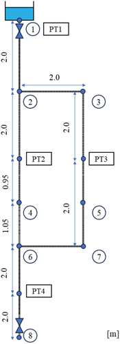
Table 1. Pipe elevation of each node and high point position for each configuration, with the high point centred in the shaded node.

Configuration	Node 1 (m)	Node 2 (m)	Node 3 (m)	Node 4 (m)	Node 5 (m)	Node 6 (m)	Node 7 (m)
C1	0	0	0	0.10	0	0	0
C2	0	0	0	0	0.10	0	0
C3	0	0	−0.03	0	0.07	0	−0.03
C4	0	0	0.03	0	0.13	0	0.03
C5	0	0	−0.03	0	0.12	0	0.03
C6	0	0	0.03	0	0.084	0	−0.03

Six pipe configurations (C1-C6) are tested, as shown in Table 1. The first two configurations (C1 and C2 schematized in Figure 1(a,b), respectively) aim to analyse the influence of the high point location in the system for the air pocket entrapment by changing the high point position from the main pipe (Node 4) to the side pipe (Node 5). The remaining four configurations aim to analyse the influence of the pipe layout elevation on the air pocket entrapment. The high point remains in the side pipe, with the centre in Node 5, but the elevations of Nodes 3 and 7 vary depending on the configuration. Details on the nodes’ elevations for the remaining configurations are presented in Table 1. Each configuration and orifice diameter have been tested four times to assess if the air entrapment phenomenon has a stochastic nature.

Four Siemens SITRANS P series Z pressure transducers with a range of 0 – 2.5 m, with a 0.5% full-scale error and a response time lower than 0.1 s are installed in the system. The first transducer, PT1, is located immediately upstream of the actuated valve to determine the initial tank head condition; PT2 and PT3 are located at half-length of the main and side pipes of the loop; and PT4 is located at mid-length of the pipe between Node 6 and the downstream end. Four transducers are installed in the pipe in the locations illustrated in Figure 1. Two types of observations are carried out: pressure-head and video recordings. All pressure-head measurements are acquired at a 1 kHz frequency. Videos are recorded using a GoPro 7 Black with a resolution of 2074 × 1520 pixels and a frame rate of 24 frames per second.

2.2. Pressure-head signals

A series of experimental tests have been conducted for six pipe configurations (C1-C6) and four orifice sizes (d = 2.2, 3.0, 4.5 and 21 mm) and each configuration-orifice size test has been repeated four times. This was done due to the uncertain nature of air entrapment and the creation of air pockets. Four repetitions demonstrated that measured air pocket volumes did not vary significantly, unlike what was observed in the single system by Ferreira et al. (2024).

Experimental pressure-head signals are present in Figure 2 for the two orifice diameters (d = 2.2 and 21 mm) and for configurations C1 and C2. The main differences in the pressure-head signals of configurations C1 and C2 include the pressurization times at each pressure transducer and the magnitude and timing of the pressure surge associated with the waterfront arrival at the downstream end. All tests start with the upstream valve opening at t = 0 s (Node 1).

Figure 2. Experimental pressure-head signals for C1 for (a) d = 2.2 and (b) d = 21 mm, and for C2 for (c) d = 2.2 mm and (d) d = 21 mm.

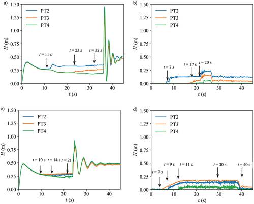
For configuration C1 with orifice d = 2.2 mm (Figure 2(a)), the air inside the pipe pressurizes simultaneously in all transducers. When the waterfront reaches PT2 at t = 11 s, the pressure-head increases due to a backward pressurization from the high point to the main pipe. Subsequent pressure-head signals steadily decrease as air is being released. Pressurization extends also to the side pipe, with water reaching PT3 at t = 23 s and PT4 at t = 32 s. A water hammer event is observed at t = 36 s when the waterfront reaches the downstream end orifice, nearly reaching a maximum value H = 1.5 m.

For configuration C1 with d = 21 mm, Figure 2(b) shows that the pressure-head signals do not increase when the upstream valve is opened (t = 0 s). The pressure-head at PT2 increases at t = 7 s since the waterfront reaches the high point in the main pipe and backward pressurizes the pipe, filling the side pipe. The water reaches PT3 at t = 17 s and PT4 at t = 20 s, considerably sooner than in C1 since the waterfront elevation does not exceed the high point during the pipe filling (unlike the case for C1 and d = 2.2 mm) and the side pipe pressurization occurs before it is completely filled. A pressure-head increase is observed around t = 22 s due to the shock between the two waterfronts (from the main pipe and side pipe), which decreases when the waterfront reaches the downstream end. No significant pressure transient is observed since there is no orifice at the downstream end.

For configuration C2 with d = 2.2 mm (Figure 2(c)), air pressurization is observed as the pressure-head increases in all pressure transducers, stabilizing when the waterfront reaches their location (PT2 at t = 10 s, PT3 at t = 14 s and PT4 at t = 21 s). The waterfront reaches PT2 before PT3 and Node 6 pressurizes before the waterfront overtops the high point in the side pipe. Similar to the configuration C1 with d = 2.2 mm (Figure 2(a)), the pressure-head increases as the waterfront reaches each transducer. The filling process continues until the waterfront reaches the downstream end at t = 24 s, 13 s sooner than in configuration C1. The generated water hammer wave amplitude and frequency are lower than in the case of configuration C1 because of the higher damping effect from a larger entrapped air pocket volume.

For configuration C2 with d = 21 mm (Figure 2(d)), the observed pressure-head has a similar behaviour as for d = 2.2 mm. The waterfront advances until it reaches PT2 and PT3, at t = 7 s and t = 9 s, respectively. The waterfront reaches the downstream end at t = 17 s, 6 s sooner than in configuration C1 due to the high point location. It is worth noting that the pressure-head drops at t = 30 s and t = 40 s, corresponding to the release of entrapped air pockets, creating small pressure-head perturbation. Once these air pockets are released, no additional local head losses exist due to the air pocket blockage and the final pressure-head decreases.

2.3. Entrapped air pocket volumes

The quantification of the entrapped air pocket volumes observed in the experimental tests is carried out by using two methods depending on the air pocket location and size. The volume of the air pockets located at the high point is quantified by cropping the images, running these through Gaussian filters to reduce image noise and binarizing to quantify the air volume of the air pocket (see Figure 3), like in the air–water interface measurements carried out in literature (Kong et al. 2019; Peddu, Chakraborty, and Das 2018). The volume of elongated air pockets outside the high point is quantified by measuring the length and the cord of each air pocket cross-section with accuracies of 1.0 and 0.1 mm, respectively. For further details, including images of pipe filling events, see Ferreira et al. (2024). Each air volume is estimated using the cross-sectional area of the air and the length of each air pocket. Since several air pockets are entrapped for each experimental test, the total air volume is obtained by the summation of individual volumes in each area, and the respective value for each configuration and orifice size is represented in Figure 4.

Figure 3. Image treatment example of air pocket volume for configuration C1 and d = 3.0 mm: (a) Original image, (b) Cropped image, (c) Image after edge detection and binarized and (d) Smoothed out image to reduce image noise.

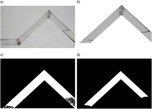
Figure 4. Experimental air pocket volumes for each configuration (C1 - C6), including the data from all repetitions.

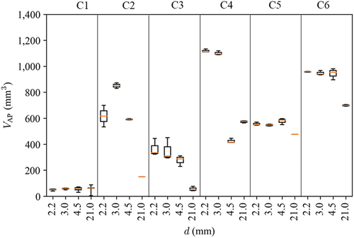
Most volumes observed in this study are higher than those reported in Ferreira et al. (2024). In previous work, air pocket formation was primarily due to flow pressurization from the high point until the downstream section of the downwards-sloped pipe. In contrast, in this study, air pocket creation results from the simultaneous pressurization of an empty section of the pipe by two different waterfronts approaching from opposing sides, creating an entrapped air pocket. Consequently, air pockets are entrapped at the high point and spread along the system.

As seen in Figure 4, configuration C1 demonstrates considerably lower entrapped air volumes than other configurations. This is due to the relatively short length of the air pocket creation zone downstream of the high point in the main pipe (Nodes 1-2-4-6-8). In this case, the air pocket is formed between the high point (Node 4) and Node 6, due to the travelling of the waterfront in the side pipe (Nodes 2-3-5-7-6) until pressurizing Node 6.

In contrast to C1, configuration C2 shows significantly higher volumes for d = 2.2, 3.0 and 4.5 mm. This is primarily because the waterfronts are not perpendicular to the pipe axis, causing the entrapment of larger air volumes. This behaviour has already been observed in single pipes by Ferreira et al. (2024).

Configuration C3 exhibits an overall lower air volume than C2. This is attributed to the main pipe filling more rapidly than the side pipe. During the filling process, when Node 6 becomes pressurized, the side pipe entraps more air despite having lower elevations.

Configuration C4 shows higher air volumes than C2 and C3 for similar orifice sizes, mainly due to the side pipe being located higher than the main pipe and air entrapped in the side pipe tends to remain there.

Configuration C5 shows larger entrapped air volumes than C3, despite both configurations having decreasing elevations in the side pipe from Node 2 to Node 3. This is because, in configuration C5, the side pipe between Node 3 to 7 rises (except in the high point zone) and, consequently, the filling process is comparatively slower than in C3 in which this pipe is horizontal and lower than the main pipe.

Configuration C6 shows lower volumes than C4 for d = 2.2 mm and 3.0 mm orifice sizes, despite higher volumes entrapped for d = 4.5 and 21 mm. This is due to the waterfront ascending from Node 2 to 3 in C6, which delays the filling process of the side pipe and does not allow air release due to the downwards-sloped pipe, unlike the horizontal side pipe in configuration C4.

Based on the analysis of above results the following additional observations can be made: (i) the smaller the orifice size is, the higher the entrapped air volume becomes because the pipe fills from bottom up and blocks the air release at the downstream end (as observed in Ferreira et al. 2024); (ii) the entrapped air volume is higher when the high point is located in the side pipe (C2-C6), because the only location where the air pocket is created is the pipe section between the downstream sloped pipe of the high point and the merging node of the loop (Node 6); (iii) the highest air pocket volumes are observed when the side pipe is located, on average, at higher elevations than the main pipe (C4 and C6), being particularly relevant for the smallest orifice diameters (d = 2.2 and 3.0 mm), which is coherent with the idea that air moves to higher elevation points; (iv) entrapped air volumes tend to be lower when the side pipe is located, on average, at lower elevations (C3 and C5), because the air ascends to the main pipe and the side pipe is filled sooner.

3. Numerical model

3.1. Original SWMM software

SWMM, typically used to simulate urban drainage and stormwater systems, is based on an implicit numerical method to solve the simplified Saint-Venant equations in a one-dimensional format. Whenever a node is pressurized, the model uses one of two methods to simulate pressurized flow (defined by the user). The first is the Extended Transport (EXTRAN) method that solves mass and momentum equations typical for pressurized pipe flows and used in EPANET software (the US-EPA’s model for pressurized pipe networks) but using SWMM’s implicit scheme and considering the flow occupies the total pipe cross-section. The second is the SLOT method, which features an artificial slot at the pipe crown with a width of 0.01D (being $\mathit{D}$ the pipe diameter) and allows the model to keep simulating the flow with Saint-Venant equations. This slot increases the storage of each section since the flow cross-section is higher than the pipe’s (Sharior, Hodges, and Vasconcelos 2023). Only the EXTRAN method is used herein since the SLOT method did not show good results when applying an air accumulator in SWMM (Ferreira et al. 2023). Further information on the general SWMM engine and its numerical implementation can be found in Rossman (2017); more details on each surcharge method can be found in Roesner et al. (1988) and in Rossman (2022). SWMM software version v5.1.015 is used since no further developments have been made regarding pipe flow rates or water depths.

3.2. AirSWMM model

The numerical model used to simulate the pipe filling process, AirSWMM, is an improvement of SWMM developed by Ferreira et al. (2024). AirSWMM is an add-on to SWMM’s source code and does not require changes in the input file. No object (e.g. pipe, node, tank) from the original SWMM was modified nor was a new object created. The modifications are carried out at the hydraulic engine by means of the implementation of an algorithm to detect entrapped air pockets to calculate their volume and pressure and to incorporate this air pressure in the flow rate and water depth calculations. Hence, the AirSWMM add-on does not require any additional input data from the user, rather than building the model with some space-time discretization constraints, i.e. a finer spatial discretization (e.g. L/D_P = 2, in this case, L = 0.042 m), to attain more accurate air pocket volume and location. This model uses the original SWMM as a baseline incorporating three main steps that require additional calculations in each time step, allowing the estimation of the air pocket location and volume. The first step checks which pipes are pressurized and updates the air pockets’ volumes being released from the system. This step also detects air volumes between two waterfronts, flagging them as entrapped air pockets. The second step incorporates the ideal gas model, relevant during the air pressurization, and the air release when orifices exist at the entrapped air location. The third step incorporates the dynamics of entrapped air pockets, namely the dragging due to the water flow rate and the air entrainment within the water flow. Some features of the last step are only activated for specific hydraulic conditions, namely: the air drag occurs when the water velocity is higher than the critical flow velocity and the air entrainment occurs when the water Froude number is above 1. In summary, the entrapped air pocket volume is obtained by the following mass balance equation:

(1) $V_{\mathit{AP},\mathit{f}}=V_{\mathit{AP},0}-\sum _{\mathit{t}=0}^t\mathit{a}{(\mathit{F}-1)}^b+\sum _{\mathit{t}=0}^t\frac{{\mathit{V}}_{\mathit{AP},\mathit{drag}}}{V_p}{Q}_w\mathit{t}$(1)

where $V_{\mathit{AP},\mathit{f}}$ and $V_{\mathit{AP},0}$ are the final and initial entrapped air pocket volumes, respectively, $\mathit{a}$ and $\mathit{b}$ are entrainment function parameters, $\mathit{F}$ is the Froude number, $V_{\mathit{AP},\mathit{drag}}/V_p$ is the air-pipe volume ratio from the small air pocket creation and $Q_w$ is the water flow rate upstream the air pocket.

In this work, AirSWMM input file from Ferreira et al. (2024), which includes pipes, tank and model parameters, is modified to account for the side pipe and different pipe elevations. All remaining input parameters are the same: the inertial damping is not considered, normal flow conditions are Froude-dominated, no variable time step is used and $\mathit{a}=2$ and $\mathit{b}=1.3$ coefficients are as previously calibrated. The pipes are discretized with a $\mathrm{\Delta x}/\mathit{D}=2$ ratio, being $\mathrm{\Delta x}$ the spatial discretization of the pipes, to maximize the entrapped air pocket volume, as calibrated in Ferreira et al. (2024). The used time step is obtained by $\mathrm{\Delta t}=0.1\mathrm{\Delta x}/\sqrt{\mathit{gD}}$ being $\mathit{g}$ the gravity acceleration, to have a Courant ($\mathit{Cr}=\mathit{c}/(\mathrm{\Delta x}/\mathrm{\Delta t})$) number below 1, being $\mathit{c}$ the pipe wave celerity. Such Courant number leads to the best compromise between numerical accuracy and computational time (J. Vasconcelos et al. 2018).

4. Results

This section compares the experimental and predicted pressure-head signals with the aim to further validate the AirSWMM model in the pipe network context (4.1). Insights on the pipe filling process and the air entrapment not described in previous studies are presented in section 4.2 and the comparison between experimental and predicted entrapped air pocket volumes and the results discussion are presented in section 4.3.

4.1. Pressure-head signals

The model is evaluated using the collected pressure-head from PT2, PT3 and PT4 for the configurations and orifice sizes presented in Figure 2 (configurations C1 and C2 for d = 2.2 and 21 mm). While the model captures the overall filling behaviour, certain numerical instabilities are noticeable when comparing numerical results to experimental data, as illustrated in Figure 5.

Figure 5. Experimental and predicted pressure-head signals in pressure transducers PT2, PT3 and PT4 for C1 with downstream orifice with d = 2.2 mm, and d = 21 mm and for C2 with downstream orifice with d = 2.2 mm, and d = 21 mm.

As it can be seen from Figure 5, in configuration C1 and orifice size of d = 2.2 mm, after the initial pressurization, the predicted pressure-head decreases until the water reaches the pressure transducers since the air release rate is low enough to create air pressurization in the pipe. However, when the waterfront reaches each transducer (at t = 13.5 s for PT2, t = 22.5 s for PT3, and t = 27 s for PT4), numerical instabilities are observed, likely due to backward pressurization within the main pipe. Further insights on the dynamics of the filling process are provided in subsection 4.2 . The pressure-head variation observed after 36 s is a consequence of the waterfront reaching the downstream end and colliding with the orifice. Although the time of waterfront arrival at the downstream end is accurately estimated, AirSWMM is not able to describe accurately the pressure transient event created. SWMM considers pipe rigid walls, and the water compressibility is simulated by the EXTRAN surcharge method. However, the pipe wave celerity in the EXTRAN surcharge method, obtained by $\mathit{c}=\mathrm{\Delta x}/\sqrt{\mathit{gD}}=0.45\mathrm{m}{\mathrm{s}}^{-1}$ (Roesner et al. 1988), is considerably lower than in plastic pipes ($\mathit{c}\approx 300\mathrm{m}{\mathrm{s}}^{-1}$). Thus, SWMM and AirSWMM using the EXTRAN surcharge method are not prepared to simulate water hammer events. SWMM’s Preissmann slot width can be adjusted to replicate the pipe wave celerity, but such modification has been shown not to provide good results while simultaneously using the air model (Ferreira et al. 2023).

In configuration C1 with d = 21 mm (see Figure 5), the orifice with the same diameter as the pipe does not restrict air release during the pipe filling. As a consequence, the air inside the pipe does not pressurize immediately after the valve opening. The estimated waterfront arrival time at each transducer is accurately predicted by the model, but the predicted pressure-heads tend to be slightly overestimated for PT3 and PT4. This is consistent with the observations by Ferreira et al. (2023) when using the original SWMM. The air pressurization feature of the AirSWMM model is not activated and hence the pressure-head and flow rate values are calculated as in the original SWMM, only tracking the location where air pockets are likely to exist.

For configuration C2 and d = 2.2 and 21 mm, similar instabilities are observed as in C1 when the waterfront reaches the transducers’ locations (see Figure 5). The waterfront arrival time at each transducer is correctly predicted, and the filling process is generally well described. However, the waterfront arrives sooner at the downstream end of the system (Node 8) than in configuration C1 since the main pipe is filled sooner. Additional insights on the pipe filling process for each configuration analysed, and the explanation for why the waterfront reaches the orifice sooner in C2 than in C1 is provided in the next section.

4.2. Pipe filling process

This subsection provides insights into how the network topography can influence the creation of air pockets. It is evident from the results shown above for different configurations that the dynamics of the pipe filling process, as well as the entrapped air pockets formation and location, are strongly influenced by the network layout and elevation. The water flows into the pipe when the upstream valve is opened at t = 0 s, primarily advancing in a pressurized flow until it reaches the junction Node 2. At this node, the waterfront divides in two fronts progressing as free surface flow in both the main and the side pipes. This is observed for all configurations with d = 2.2 mm (exemplified in Figures 5 and 6 for C1 and C2) until t = 9.4 s when the specific pipe layout begins to influence the pipe filling process.

Figure 6. Snapshots of the predicted pipe filling process in Configuration C1 with d = 2.2 mm at different filling times and the final steady state when air pocket is fully formed.

The progression of waterfronts during the filling process for configuration C1 and orifice d = 2.2 mm is schematically illustrated in Figure 6 for five snapshots in time. As seen from this figure, as the waterfront reaches the rising pipe immediately upstream Node 4, considerable changes occur in the system. At t = 14 s, the flow in the main pipe generates a backward pressurization process in the main pipe which propagates into the side pipe. Subsequently, at t = 26 s, the side pipe fills with water until the waterfront reaches Node 5. The side pipe becomes fully pressurized and the developing free surface flow, predicted after the high point within the main pipe, gives rise to an entrapped air pocket. At t = 29.2 s, the waterfront continues its progression towards the downstream end, ultimately reaching the orifice at Node 8 at t = 35.6 s. At this time, the pipe filling process has concluded, culminating in a water hammer event created by the waterfront collision with the orifice at the downstream pipe end. Entrapped air pockets remain in the pipe even after the filling process has finished, making it necessary to have the pipe pressurized for a long period and with high pressure for the air to dissolve or mix in the water and be ultimately drained out. As it can be seen from Figure 6 for t = 36.5 s, the predicted location of the air pocket corresponds to the experimentally observed one. Additional entrapped air pockets are predicted in the side pipe by the model but are not observed in the experiments. However, the predicted additional pockets, originating from the numerical instabilities during the pipe filling process, are very small (4 mm³), i.e. negligible when compared to the volume of the actual air pocket (50 cm³).

The filling process in Configuration C2 with d = 2.2 mm (Figure 7) is different from the one observed in C1 after t = 9.4 s. At t = 14 s, the water does not ascend in the rising pipe of the high point but continues to advance along the main pipe. When reaching the junction at Node 6, the waterfront divides into two: one front progresses towards the downstream end (Node 8), while the other front fills the side pipe in the opposite direction than in C1 (from Node 6 to 7). At t = 18 s, the waterfront coming from Node 3 in the side pipe reaches the rising pipe of the high point. This pressurizes the water column upstream, which was initially a free-surface flow, resulting in the formation of the observed entrapped air pocket. Subsequently, the waterfront ascends the high point and overcomes, appearing as a continuous free surface flow from the high point until the junction Node 6. At t = 18 s, i.e. the moment just before the pipe between Nodes 6 and 7 pressurizes, an air pocket is created from Node 5 to Node 6. At t = 29.2 s, the water column pressurizes in a reverse direction, moving towards Node 7 in a downstream direction (since Node 7 has not yet pressurized). At the final steady state condition in the system (t = 35.6 s), major differences between predicted and observed can be seen, as opposed to configuration C1 where the waterfront had already reached the downstream end at this point.

Figure 7. Snapshots of the predicted pipe filling process in Configuration C2 with d = 2.2 mm at different pipe filling times and the final steady state experimental air pocket location.

Despite the predicted and the experimentally measured air pockets being located in the same areas of the pipe system, two main differences should be highlighted. Firstly, the experimental total air pocket volume (840 cm³) exceeds the predicted one (300 cm³). The lack of air entrainment was also observed during the experimental testing, explaining the relatively minor variation in air pocket volumes as depicted in Figure 4.

4.3. Air pocket volumes

Figure 8 presents the experimental and predicted air pocket volumes obtained at the final steady state in the analysed pipe network for six different configurations and four orifice sizes, with each experiment repeated four times.

Figure 8. Comparison between experimental and predicted air pocket volumes.

Two main observations can be drawn from these results. Firstly, experimental air volumes show some variability for the same configuration-orifice size test due to the randomness of the filling process, whereas only one predicted air volume is obtained given the deterministic nature of the AirSWMM model. Secondly, the results obtained are somewhat mixed in terms of prediction accuracy. The model predicted reasonably well air pocket volumes for configurations C1 and C6 for most orifice sizes but underestimated air pocket volumes for configurations C2, C3, C4 and C5 for most (in some cases) orifice sizes, in some cases quite substantially. A more detailed analysis of the results is presented for each configuration in the following text.

For Configuration C1, air pockets are comparatively small to the remaining configurations, with volumes lower than 100 cm³, and restricted to the high point location. The AirSWMM model is capable of predicting air pocket volume with a maximum relative error ε_r^max, of 25%, which is of the same order of magnitude as results obtained in the single pipe presented in Ferreira et al. (2024).

For Configuration C2, experimental pocket air volumes range between 180 and 950 cm³, decreasing with the orifice size increase, and the model significantly underpredicts these volumes, not leading to volumes higher than 300 cm³, i.e. an error of ε_r^max = 83%. This is because the model more easily creates air pockets in the high points due to the considerable elevation differences whilst their creation is generally more difficult in horizontal or low-slopped pipes because of the steeper wavefront. Nevertheless, as exemplified in Figures 6 and 7, estimated air pockets are created at the high point and along the pipe in the same locations as observed in experimental tests.

For Configuration C3, experimental air volumes are lower than those for configuration C2, ranging from 80 to 420 cm³ since the side pipe is positioned 3 cm below the main pipe. The air pocket volume is underestimated by the numerical model for smaller orifice diameters (d = 2.2, 3.0 and 4.5 mm) with ε_r^max = 65%, whereas, for the system without the orifice (d = 21 mm), ε_max increases to 280%; this is because the actual air pocket volume for d = 21 mm is quite small (42–50 cm³) in comparison with those from other tests for C3 (220–450 cm³), suggesting that the numerical model is more sensitive to the network elevation than to the filling rate conditions.

For Configuration C4, with the side pipe raised by 3 cm above the main pipe, the experimental air volumes reach their highest values, ranging from 410 to 1080 cm³. Air volumes are better estimated (ε_r^max = 45%) than for the previous two configurations (C2, C3) since the waterfront principally progresses in the main pipe and the side pipe remains mostly empty during the filling process, both in the experimental tests and in the numerical model, leading to good air volume estimates.

The air pocket volumes for Configuration C5 present a narrow range from 475 to 600 cm³, despite being relatively high volumes in absolute terms. Predicted values range from 100 to 320 cm³, with ε_r^max = 80%. This underprediction is likely due to the same reasons as in C3, that is the numerical model being more sensitive to the network elevation than to the filling rate. However, the experimental air volume for d = 21 mm hardly varies since air is only entrapped at the high point.

For Configuration C6, air volumes show a wide variation, ranging from 720 to 1050 cm³. Unlike other configurations, the model is capable of accurately predicting air pocket volumes (900–1000 cm³) for smaller orifices sizes (d = 2.2 – 4.5 mm) with ε_r^max = 9%. However, for d = 21 mm, the experimental and predicted volumes differ significantly, with values of 720 cm³ and 160 cm³, respectively (ε_r^max = 82%). Higher estimate accuracies for smaller orifices are associated with lower flow rates, being entrapped air volume mainly conditioned by the slope of the pipe. The numerical model seems to simulate better downwards-sloped pipes than rising pipes (like in C5) for these flow rates. The worst estimate is associated with the highest flow rate, where the pipe slope is not as relevant in the creation of entrapped air pockets.

Overall, smaller air pockets are more accurately predicted, especially when the air pocket is confined to the high point location. Opposite of this, air pocket volumes are considerably overestimated when the air pockets are elongated and spread along the pipes. Conversely, larger air pocket volumes tend to be mostly underestimated. There are several reasons for AirSWMM to consistently underpredict entrapped air pocket volumes and to have different air pocket lengths.

Firstly, the model predicts steeper waterfront slopes in comparison with those observed in experimental conditions. As waterfronts push air to the downstream end of the pipe system, this results in less predicted air volume than the actually entrapped. The objective of this research is to detect and quantify entrapped air pocket volumes using a set of valid assumptions for 1-D solvers rather than targeting a more accurate but complex 3D analyses, which are impractical in standard water distribution problems. Thus, minor modifications were incorporated in the original SWMM code to account for the air phase in water flow rate and depth calculations, and these are not sufficient to describe the observed waterfront propagation and, consequently, the accurate estimate of the final volumes.

Secondly, the AirSWMM model cannot reproduce the exact air pocket length and depth at the final steady state. This is mainly due to simplifications associated with the 1D model used (e.g. air pocket geometrical representation, surface tension, etc.) which do not allow to describe the 3D nature of the observed phenomena. In fact, the shape and length of air pockets vary with pressure, volume and incoming flow (Perron, Kiss, and Poncsák 2006). However, this behaviour cannot be incorporated into the AirSWMM model, which was deliberately kept simple, as a (modified) 1D model. Therefore, AirSWMM is not able to reproduce the angle of the air pockets with the pipe wall resulting in different air pocket lengths than the actual ones. Still, despite the underestimation of air pocket volume and length, the AirSWMM model is a step ahead in the determination of the approximate locations and sizes of the air pockets.

5. Discussion

AirSWMM allows to determine the accurate location of the air pockets, though the air pocket volumes are not accurately predicted for all configurations-orifice sizes. The air pocket volume is well estimated when it is limited to a small length of the pipe, it is overestimated when the volume is small and spread along the pipe and underestimated for larger air volumes, also spread along the pipe. AirSWMM uses the SWMM engine for calculating flow rates and pressure-heads and has additional features to compute, in a simply coupled way, the air–phase interaction at each time step. Entrapped air pocket volumes strongly depend on the water depths calculated by the SWMM engine at each node, during the pipe filling process. A more accurate air pocket volume estimation would require modifying the core components of the SWMM engine, which was not the purpose of this research. Thus, users should be aware of the limitations of the AirSWMM model, when estimating the air pocket volumes. Additionally, the model prediction of the air pocket shape does not correspond to that of the experimental observations with shorter air pocket lengths predicted than observed. Nevertheless, AirSWMM can be used to identify the likely locations of air pockets hence, in turn, the best locations for air release devices. It can also be used to determine locations where the pipe layout could be optimised to improve the operation during IWS.

AirSWMM can also be useful for improving the operation of IWS systems. Firstly, AirSWMM allows a better estimation of pipe filling times in comparison with the original SWMM. This is because the presence of air in the system delays the pipe filling process and the incorporation of the air-water interaction in AirSWMM allows a better description of existing phenomena. Secondly, SWMM provides an overestimate of the pressure-heads because it does not incorporate entrapped air pockets’ local head losses, whereas AirSWMM provides a more realistic estimate of pressure-heads along the pipes. This is because the head losses created by entrapped air pockets are partially accounted for in the AirSWMM through higher friction in wet perimeters, along the air pocket lengths (Ferreira et al. 2024). Thirdly, a better description of pressure distribution along the pipe network during IWS operation will help to identify with higher accuracy the pipe locations with lower pressure, providing, therefore, a better assessment of potential intrusion or cross-contamination risk assessment. Finally, AirSWMM allows quantifying the flow rate of air being released at each system orifice which cannot be done by the SWMM. Such quantification can help utilities to assess which domestic flowmeters should be more frequently replaced, since running dry wears the meters faster than under continuous water supply (Ferrante et al. 2022).

6. Conclusions

New experimental tests have been conducted to better understand the entrapped air pocket formation at high points in the pipe network, including the influence of network topography and the filling rate on the air pocket location and volume. The previously developed AirSWMM model (Ferreira et al. 2024) which was developed and validated for a single pipe configuration is tested herein in a single loop network at a laboratory scale with varying pipe elevations and filling rates.

Based on the experimental and modelling results obtained, the following conclusions are made:

• Experiments have revealed that air pocket volumes and shapes strongly depend on the location of the high point in the network, the pipe slopes and the water filling rate. It was observed that entrapped air volumes can be up to 100 times higher when the high point is located in the side pipe than when it is located on the main pipe. It was also observed that air pocket volumes tend to decrease with the increasing water filling rate, which is determined by downstream orifice size, a finding consistent with Ferreira et al. (2024). Finally, experimental observations provide evidence that air pocket creation and final volumes are dominated by the waterfront division and merging at network node junctions and the waterfront progression along the multiple pipes, despite the processes also having a stochastic nature.

• AirSWMM has shown a good prediction capability for the water filling behaviour, with and without air pressurization, for the tested pipe network. Some numerical instabilities were observed when the waterfront reaches each node, but this does not affect the prediction of the overall filling process nor the arrival time at the downstream end of the system.

• AirSWMM model also predicts well the air pocket network location in all cases, allowing the use of such predictions to support or complement the recommendations from the American Water Works Association (2016) and Deltares (2016) on where air release devices should be installed.

• AirSWMM model tends to over-predict the volume of smaller and elongated air pockets, whereas smaller and concentrated air pockets are predicted reasonably well, with a 25% relative error. AirSWMM can both correctly predict (with ε_r^max = 10%) or under-predict larger air pocket volumes (with ε_r^max = 90% of the observed values, depending on the pipe configuration and elevations. The inaccuracies in predictions arise mainly from the simplified single-phase 1D flow modelled by the AirSWMM, whereas the real flow is multi-phase 3D.

Collected experimental data can be used as a benchmark data set for further numerical developments.

Additional experimental tests, with a broader range of pipe diameters, similar to those conducted by Guizani et al. (2006) on waterfront slopes during pipe-filling events, are recommended to better describe pipe filling processes in numerical models. Future research should focus on using three-dimensional computational fluid dynamics (3D CFD) models for the simulation of pipe filling stages considering the geometrical shape of the pipe and water surface tension to better describe the waterfront propagation and the entrapped air pocket’s volumes, shape and length. Combining 1D and 3D CFD models should also be focused on considering the local diagnosis of systems and post-accident analyses. This work did not consider the existence of water demand throughout the pipe system, which is likely to influence the overall filling process dynamics. Water demand could be implemented with already existing SWMM elements as proposed by Campisano, Gullotta, and Modica (2019) or directly in the source code. Experimental tests with water demand at different nodes should be carried out in the future (supported by the corresponding numerical tests) as these may influence the formation of air pockets. In addition, the influence of user’s private tanks on the formation of entrapped air pockets should also be carried out.

Disclosure statement

No potential conflict of interest was reported by the author(s).

Data availability statement

The data that support the findings of this study are available from the corresponding author, J. Ferreira, upon reasonable request.

Additional information

Funding

The authors acknowledge the Portuguese national funding agency, Fundação da Ciência e Tecnologia (FCT), for funding the reported work within grant number [SFRH/BD/146709/2019] and for the support through funding UIDB/04625/2020 to the research unit CERIS.

References

- Ballun, John V. 2016. Air Valves: Air-Release, Air/Vacuum and Combination. 2nd ed. Denver, CO, USA: American Water Works Association, AWWA.
- Benjamin, T. Brooke. 1968. “Gravity Currents and Related Phenomena.” Journal of Fluid Mechanics 31 (2): 209–248. https://doi.org/10.1017/s0022112068000133.
- Cabrera-Bejar, J. A., and V. G. Tzatchkov. 2009.” Inexpensive Modeling of Intermittent Service Water Distribution Networks.” Paper Presented at the World Environmental and Water Resources Congress 2009: Great, Rivers Kansas City, Missouri, May 17-21.
- Campisano, Alberto, Aurora Gullotta, and Carlo Modica. 2019. “Using EPA-SWMM to Simulate Intermittent Water Distribution Systems.” Urban Water Journal 15 (10): 925–933. https://doi.org/10.1080/1573062x.2019.1597379.
- Christodoulou, S., and A. Agathokleous. 2012. “A Study on the Effects of Intermittent Water Supply on the Vulnerability of Urban Water Distribution Networks.” Water Science & Technology: Water Supply 12 (4): 523–530. https://doi.org/10.2166/ws.2012.025.
- Christodoulou, Symeon E., Chrystalleni Christodoulou, and Agathoklis Agathokleous. 2017. “Influence of Intermittent Water Supply Operations on the Vulnerability of Water Distribution Networks.” Journal of Hydroinformatics 19 (6): 838–852. https://doi.org/10.2166/hydro.2017.133.
- Davies, R. M., and Geoffrey Ingram Taylor. 1950. “The Mechanics of Large Bubbles Rising Through Extended Liquids and Through Liquids in Tubes.” Proceedings of the Royal Society of London Series A, Mathematical and Physical Sciences 200 (1062): 375–390. https://doi.org/10.1098/rspa.1950.0023.
- Dumitrescu, D. T. 1943. “Strömung an einer Luftblase im senkrechten Rohr.” ZAMM - Journal of Applied Mathematics and Mechanics/Zeitschrift für Angewandte Mathematik und Mechanik 23 (3): 139–149. https://doi.org/10.1002/zamm.19430230303.
- Escarameia, Manuela. 2004. Experimental and Numerical Studies on Movement of Air in Water Pipelines. In: HR Wallingford.
- Ferrante, Marco, Dewi Rogers, Josses Mugabi, and Francesco Casinini. 2022. “Impact of Intermittent Supply on Water Meter Accuracy.” Journal of Water Supply: Research and Technology-Aqua 71 (11): 1241–1250. https://doi.org/10.2166/aqua.2022.091.
- Ferreira, João P., Norma Buttarazzi, David Ferras, and Dídia I. C. Covas. 2021. “Effect of an Entrapped Air Pocket on Hydraulic Transients in Pressurized Pipes.” Journal of Hydraulic Research 59 (6): 1018–1030. https://doi.org/10.1080/00221686.2020.1862323.
- Ferreira, J. P., D I C Covas David Ferras, and Z. Kapelan. 2022. “Modelling of Air Pocket Entrapment During Pipe Filling in Intermittent Water Supply Systems.” Paper presented at the 2nd International Joint Conference on Water Distribution Systems Analysis & Computing and Control in the Water Industry (WDSA/CCWI), Valencia, Spain, 18-22 July.
- Ferreira, João P, D I C Covas David Ferras, J. A. van der Werf, and Z. Kapelan. 2024. “Air Entrapment Modelling During Pipe Filling Based on SWMM.” Journal of Hydraulic Research 62 (1): 39–57. https://doi.org/10.1080/00221686.2024.2305354.
- Ferreira, João P., David Ferras, Dídia I. C. Covas, and Zoran Kapelan. 2023. “Improved SWMM Modeling for Rapid Pipe Filling Incorporating Air Behavior in Intermittent Water Supply Systems.” Journal of Hydraulic Engineering 149 (4): 04023004. https://doi.org/10.1061/jhend8.Hyeng-13137.
- Freni, Gabriele, Mauro De Marchis, and Enrico Napoli. 2014. “Implementation of Pressure Reduction Valves in a Dynamic Water Distribution Numerical Model to Control the Inequality in Water Supply.” Journal of Hydroinformatics 16 (1): 207–217. https://doi.org/10.2166/hydro.2013.032.
- Gandenberger, Wilhelm. 1957. Über die wirtschaftliche und betriebssichere Gestaltung von Fernwasserleitungen. München: Oldenbourg.
- Goldring, B. T. 1979. “The Use of Small-Scale Siphon Models.” Proceedings of the Institution of Civil Engineers 67 (4): 929–942. https://doi.org/10.1680/iicep.1979.2782.
- Guizani, Mokhtar, Jose Vasconcelos, Steve J. Wright, and Khlifa Maalel. 2006. “Investigation of Rapid Filling of Empty Pipes.” Journal of Water Management Modeling R225-20:463–482. https://doi.org/10.14796/jwmm.R225-20.
- Kong, Ran, Adam Rau, Seungjin Kim, Stephen Bajorek, Kirk Tien, and Chris Hoxie. 2019. “A Robust Image Analysis Technique for the Study of Horizontal Air-Water Plug Flow.” Experimental Thermal & Fluid Science 102:245–260. https://doi.org/10.1016/j.expthermflusci.2018.12.001.
- Lauchlan, C. S., M. Escarameia, R. W. P. May, R. Burrows, and C. Gahan. 2005. Air in Pipelines, A Literature Review. In: HR Wallingford.
- Liou, C. P., and W. A. Hunt. 1996. “Filling of Pipelines with Undulating Elevation Profiles.” Journal of Hydraulic Engineering 122 (10): 534–539. https://doi.org/10.1061/(ASCE)0733-9429(1996)122:10(534).
- Lubbers, C. L., and F. Clemens. 2006. “Breakdown of Air Pockets in Downwardly Inclined Sewerage Pressure Mains.” Water Science Technology 54 (11–12): 233–240. https://doi.org/10.2166/wst.2006.769.
- Marchis, M., C. M. Fontanazza, G. Freni, G. La Loggia, E. Napoli, and V. Notaro. 2010. “A Model of the Filling Process of an Intermittent Distribution Network.” Urban Water Journal 7 (6): 321–333. https://doi.org/10.1080/1573062X.2010.519776.
- Martin, C. S. “1976. Entrapped Air in Pipelines.” Paper presented at the Second International Conference on Pressure Surges, London, England.
- Martins, Nuno M. C., J. N. Delgado, H. M. Ramos, and D. I. C. Covas. 2017. “Maximum Transient Pressures in a Rapidly Filling Pipeline with Entrapped Air Using a CFD Model.” Journal of Hydraulic Research 55 (4): 506–519. https://doi.org/10.1080/00221686.2016.1275046.
- Peddu, Akhilesh, Shubhankar Chakraborty, and Prasanta Kr. Das. 2018. “Visualization and Flow Regime Identification of Downward Air–Water Flow Through a 12 mm Diameter Vertical Tube Using Image Analysis.” International Journal of Multiphase Flow 100:1–15. https://doi.org/10.1016/j.ijmultiphaseflow.2017.11.016.
- Perron, A., L. I. Kiss, and S. Poncsák. 2006. “An Experimental Investigation of the Motion of Single Bubbles Under a Slightly Inclined Surface.” International Journal of Multiphase Flow 32 (5): 606–622. https://doi.org/10.1016/j.ijmultiphaseflow.2006.02.001.
- Pothof, Ivo, and Francois Clemens. 2010. “On Elongated Air Pockets in Downward Sloping Pipes.” Journal of Hydraulic Research 48 (4): 499–503. https://doi.org/10.1080/00221686.2010.491651.
- Pothof, I. W. M., and F. H. L. R. Clemens. 2011. “Experimental Study of Air–Water Flow in Downward Sloping Pipes.” International Journal of Multiphase Flow 37 (3): 278–292. https://doi.org/10.1016/j.ijmultiphaseflow.2010.10.006.
- Roesner, L. A., J. A. Aldrich, R. E. Dickinson, and T. O. Barnwell. 1988. Storm Water Management Model user’s Manual, Version 4: EXTRAN Addendum. In: U.S. Environmental Protection Agency.
- Rossman, L. A. 2022. Addendum to the Storm Water Management Model Reference Manual, Volume II – Hydraulics. In: U.S. Environmental Protection Agency.
- Rossman, Lewis A. 2017. Storm Water Management Model Reference Manual Volume II – Hydraulics. In: U.S. Environmental Protection Agency.
- Sharior, Sazzad, Ben R. Hodges, and Jose G. Vasconcelos. 2023. “Generalized, Dynamic, and Transient-Storage Form of the Preissmann Slot.” Journal of Hydraulic Engineering 149 (11): 04023046. https://doi.org/10.1061/jhend8.Hyeng-13609.
- Simukonda, Kondwani, Raziyeh Farmani, and David Butler. 2018. “Intermittent Water Supply Systems: Causal Factors, Problems and Solution Options.” Urban Water Journal 15 (5): 488–500. https://doi.org/10.1080/1573062x.2018.1483522.
- Tukker, Michiel, Kees Kooij, and Ivo Pothof. 2016. Hydraulic Design and Management of Wastewater Transport Systems. IWA Publishing. https://doi.org/10.2166/9781780407814
- Vasconcelos, Jose, Yasemin Eldayih, Yang Zhao, and Jalil A. Jamily. 2018. “Evaluating Storm Water Management Model Accuracy in Conditions of Mixed Flows.” Journal of Water Management Modeling 27 (C451): 1–10. https://doi.org/10.14796/jwmm.C451.
- Vasconcelos, Jose G., and Gabriel M. Leite. 2012. “Pressure Surges Following Sudden Air Pocket Entrapment in Storm-Water Tunnels.” Journal of Hydraulic Engineering 138 (12): 1081–1089. https://doi.org/10.1061/(asce)hy.1943-7900.0000616.
- Vasconcelos, Jose G., and Davi T. Marwell. 2011. “Innovative Simulation of Unsteady Low-Pressure Flows in Water Mains.” Journal of Hydraulic Engineering 137 (11): 1490–1499. https://doi.org/10.1061/(asce)hy.1943-7900.0000440.
- Vasconcelos, Jose G., Steven J. Wright, and P. L. Roe. 2006. “Improved Simulation of Flow Regime Transition in Sewers: Two-Component Pressure Approach.” Journal of Hydraulic Engineering 132 (6): 553–562. https://doi.org/10.1061/(ASCE)0733-9429(2006)132:6(553).
- Walski, Thomas M., Tad S. Barnhart, John M. Driscoll, and Richard M. Yencha. 1994. “Hydraulics of Corrosive Gas Pockets in Force Mains.” Water Environment Research 66 (6): 772–778. https://www.jstor.org/stable/25044480.
- Walter, David, Miran Mastaller, and Philipp Klingel. 2017. “Accuracy of Single-Jet Water Meters During Filling of the Pipe Network in Intermittent Water Supply.” Urban Water Journal 14 (10): 991–998. https://doi.org/10.1080/1573062x.2017.1301505.
- Zhou, F., F. E. Hicks, and P. M. Steffler. 2002. “Transient Flow in a Rapidly Filling Horizontal Pipe Containing Trapped Air.” Journal of Hydraulic Engineering 128 (6): 625–634. https://doi.org/10.1061//asce/0733-9429/2002/128:6/625.
- Zhou, Ling, Deyou Liu, and Bryan Karney. 2013. “Investigation of Hydraulic Transients of Two Entrapped Air Pockets in a Water Pipeline.” Journal of Hydraulic Engineering 139 (9): 949–959. https://doi.org/10.1061/(asce)hy.1943-7900.0000750.