How do psychological and physiological performance determinants interact within individual athletes? An analytical network approach

ABSTRACT

Previous research on sports performance has mostly been conducted: (a) at a single point, or at most, a few points in time, (b) at the group level, and (c) as a causal chain of monodisciplinary predictor and outcome variables. In the present research, we argue and demonstrate that the next important step should be to monitor, analyze, and visualise the dynamic and individual-specific interactions of multidisciplinary determinants of sports performance. Hence, we apply a recently developed analytical approach, that is, (Time-Varying) Vector-AutoRegressive ((TV)-VAR) modelling, which captures the intra-individual interactions and changes of multidisciplinary determinants. We first measured critical psychological (e.g., self-efficacy) and physiological (e.g., heart rate) factors among youth male football (soccer) players at a professional club, on a daily basis across one season. Next, we assessed the temporal dynamics of the factors with (TV-)VAR models and visualised the findings in network graphs. We present the results of two show-cases that demonstrate how multidisciplinary key determinants of sports performance can dynamically evolve across a sports season, that is, interact and change in individual-specific ways over time. Specifically, the results of Player 1 revealed a stable network across the season in which self-efficacy was the strongest predictor of other determinants, whereas this was not the case for Player 2. These new insights improve our understanding of how key determinants of sports performance are dynamically related within individual athletes and may allow practitioners to develop and implement person-specific, targeted, and timely interventions.

KEYWORDS:

• Graph theory
• personalised approach
• soccer performance
• time series analysis
• within-person dynamics

Introduction

Elite athletes across various sports are striving toward performance optimisation and excellence. Therefore, scholars and practitioners from the fields of psychology and sports sciences have attempted to identify the underlying key determinants to support athletes in performing optimally. Previous literature has mostly examined the role of these determinants: (a) at a single point, or at most, a few points in time, (b) at a group level, and (c) as a causal chain of monodisciplinary predictor and outcomes variables (Davids et al., 2003; Glazier et al., 2003; Phillips et al., 2010). More recently, researchers have suggested that those determinants may rather interact in individual-specific, complex ways over time (Davids et al., 2014; Den Hartigh et al., 2017, 2018; Glazier, 2017; Neumann et al., 2021; Williams et al., 2020). The purpose of the present research is therefore to argue and demonstrate that the next important step should be to understand the dynamic and individual-specific interactions of multidisciplinary key determinants of sports performance. Such an approach has consequences for the way data needs to be collected and analyzed. We, therefore, apply (Time-Varying) Vector-AutoRegressive ((TV)-VAR) modelling (Bringmann et al., 2018), which allows us to examine the temporal order of dynamic relationships among key determinants of performance in a sports context. This novel approach can improve our understanding of how determinants are dynamically related in individual athletes, and accordingly, provides suggestions for athlete-specific interventions to optimise sports performance.

Within the scope of this article and in accordance with the latest developments, we refer to sports performance as an emerging process governed by individual-specific, interacting biopsychosocial factors (Den Hartigh et al., 2017; Glazier, 2017; Hill et al., 2018a; Neumann et al., 2021). In the next sections, we will subsequently argue why acknowledging (a) the dynamics, (b) individual-specificity, and (c) interactions of key determinants of performance is an important avenue to move forward in research and practice. Then, we will present the recently developed (TV-)VAR modelling approach and explain how we apply this method to data of professional football (soccer) players.

Dynamics

During matches, sports seasons, and careers, the state of an athlete evolves and undergoes changes. This means that the state at a given moment is not only a function of a positive or negative event encountered but also of the previous state(s), which is referred to as iterativity or temporal dependence (Briki et al., 2013; Den Hartigh et al., 2014; Den Hartigh, Van Geert, et al., 2016; Gernigon et al., 2010; Hill et al., 2018a, 2018b; Salmon & McLean, 2020). For instance, research showed that an athlete’s motivation during a match is influenced by motivational states in previous matches (Blanchard et al., 2007). Relatedly, in the field of sports sciences, the perceived exertion at one point may influence the subsequent perception of exertion and recovery (Jones et al., 2017; Moalla et al., 2016). Important to note is that those temporal dynamics may also change over time. In an illustrative study, Van der Sluis et al. (2019) demonstrated that the level of, for instance, self-efficacy of a talented athlete changed across a sports season. In fact, it peaked after playing well in tournaments and was at its lowest when being sick, playing badly at tournaments, and receiving negative performance feedback from her parents. Moreover, studies showed that self-efficacy and performance are interconnected and may influence each other in an upward spiral, but may subsequently change into a downward spiral (Moritz et al., 2000). For example, if self-efficacy constantly increases and leads to a state of over-confidence, the link between self-efficacy and performance may turn into a negative one (Stone, 1994; Vancouver et al., 2002).

Despite the dynamic nature of performance determinants, the great majority of research has studied samples of athletes at a single point, or at most a few points in time, which limits our understanding of how determinants of sports performance dynamically evolve in individual athletes (Davids et al., 2003; Den Hartigh et al., 2017; Den Hartigh, Van Geert, et al., 2016). Statistical models that are based on averages simply display the average relation between the determinants and do not detect changes in strength or direction over time. Capturing changing dynamics is important since it could help researchers and practitioners to detect, or even anticipate, tipping or transition points from one phase to another, such as from optimal performance to under-achievement (Hill et al., 2020; Scheffer et al., 2018). In order to understand the (changing) dynamics of key determinants of sports performance, such as self-efficacy, motivation, exertion, and recovery, these factors must be measured repeatedly.

Individual-specificity

As researchers, we are interested in how key determinants of sports performance dynamically develop across time within individuals, and how this can be modelled (Bailey, 2019; Bartlett et al., 2017; Robertson et al., 2017; Thornton et al., 2019). Practitioners want to know which factors to intervene on for which athlete, to optimise performance. In previous research (e.g., Barte et al., 2019; Fletcher & Sarkar, 2012; Moalla et al., 2016), however, associations between key determinants are typically based on scores of groups of athletes. A disadvantage of this approach is that models based on group-level analysis only generalise to individuals if the process of investigation is ergodic (Birkhoff, 1931), which is typically not the case (Fisher et al., 2018; Hill et al., 2021; Mangalam & Kelty-Stephen, 2021; Molenaar & Campbell, 2009). Ergodicity entails that the processes and the related statistical characteristics, such as mean and variance, remain stable over time (also referred to as “Stationarity”) and that the same statistical model applies to the data of all participants within a particular sample or population (also referred to as “Homogeneity”).

As an illustration, a recent study among football players of a professional youth academy tested the assumption of homogeneity by comparing group-level and individual-level statistics of load and recovery scores (Neumann et al., 2021). The results showed that standard deviations and correlations between load and recovery found at the team level did not generalise to the individual players within the teams. This nonergodicity is not unique to the sports context; It has also been found in research on personality and affect dynamics, for instance (e.g., Fisher et al., 2018; Molenaar & Campbell, 2009). Hence, increasing our understanding of the dynamic process of change requires an individual-level approach.

Interactions of multidisciplinary factors

Previous research further suggests that performance determinants tend to interact continuously (Davids et al., 2003, 2005; Den Hartigh et al., 2017; Hill et al., 2018a; Lames & McGarry, 2007). To be more specific, Phillips et al. (2010) indicate that we should shift toward a multidisciplinary and integrative perspective to better understand how multiple interacting factors shape expert performance. The authors argue that the same performance outcome can be achieved in different ways as it emerges from interactions between the person and the environment. Accordingly, Glazier (2017) developed a Grand Unified Theory, which supports the notion that sports performance is governed by complex interactions of factors from multiple disciplines (e.g., psychology, physiology, and biomechanics). In line with these theoretical perspectives, Den Hartigh and colleagues (2016, 2018) considered excellent human performance from a dynamic network model, which aims at capturing the numerous interacting factors at the individual level. Using computer simulations, the authors showed how a network of different (e.g., psychosocial, environmental) variables changing over time, could predict typical individual developmental patterns towards excellent performance. However, as stressed in the recent review by Zentgraf and Raab (2023), interactions between important multidisciplinary factors underlying sports performance have not yet been investigated in real-world sports settings. The authors further emphasised that interactions can be bi-directional, and that models should be able to treat factors as predictor and outcome variables. Hence, there is a need for tools to analyse interactions within and between empirically collected multidisciplinary factors that shape sports performance, which will be discussed next.

(TV-)VAR modelling

VAR modelling is a statistical technique that uses regression equations to model the structure of the time dependency for multiple time series (Rosmalen et al., 2012). It was developed for research in econometrics and has been applied to fields such as sociology, meteorology, political sciences, neuroimaging, and psychology (Bringmann et al., 2016; Rosmalen et al., 2012; Van der Krieke et al., 2016). The model reveals autoregressive effects (i.e., to what extent a factor is predictive of itself over time) and cross-lagged effects (i.e., to what extent a factor is predictive of other factors over time). Consider, for example, a bivariate VAR model: (1) $\begin{array}{rl}{y}_{1,t}& ={\beta }_{10}+{\beta }_{11}{y}_{1,t-1}+{\beta }_{12}{y}_{2,t-1}+{\epsilon }_{1,t}\\ y_{2,t}& ={\beta }_{20}+{\beta }_{21}{y}_{1,t-1}+{\beta }_{22}{y}_{2,t-1}+{\epsilon }_{2,t}\end{array}$(1) In the model there are y_i,t variables, where i = 1, 2, … , m is the number of variables and t is the time index. The β_i0 (i = 1 or 2) coefficients represent the intercept of the model. The dependent variable (e.g., y_1,t, y_2,t) is regressed on its lagged values (y_1,t-1 and y_2,t-1) through the autoregressive parameters (β₁₁ and β₂₂) and the lagged values of each of the other dependent variables (y_2,t-1 and y_1,t-1) through the cross-lagged parameters (β₁₂ and β₂₁). The innovation terms ϵ_1,t and ϵ_2,t are those parts of the current observations y_1,t and y_2,t that cannot be explained by previous observations (y_1,t-1 and y_2,t-1).

TV-VAR modelling was recently developed by Bringmann et al. (2018), and is an extension of the standard VAR approach (see also Albers & Bringmann, 2020; Bringmann et al., 2017; Haslbeck et al., 2020). This extension can additionally account for nonstationarity in the data, by allowing the β coefficient to vary over time (details and validation can be found in Bringmann et al., 2018).¹ Using the example above, a bivariate TV-VAR model is defined as: (2) $\begin{array}{rl}{y}_{1,t}& ={\beta }_{10,t}+{\beta }_{11,t}{y}_{1,t-1}+{\beta }_{12,t}{y}_{2,t-1}+{\epsilon }_{1,t}\\ y_{2,t}& ={\beta }_{20,t}+{\beta }_{21,t}{y}_{1,t-1}+{\beta }_{22,t}{y}_{2,t-1}+{\epsilon }_{2,t}\end{array}$(2) Different to the standard VAR, the intercept and the direction and strength of the autoregressive and cross-lagged effects can now vary over time (i.e., take different values). A simulation study by Bringmann et al. (2018) has shown that when the dynamics of the data is time-invariant, the VAR model shows better results. On the contrary, when the dynamics of the data are time-varying, the TV-VAR model performs better than the VAR model.

A straightforward way to display these effects is to graphically visualise them in a network (Bringmann et al., 2016; Van der Krieke et al., 2016). In a network graph, each node represents a performance determinant (e.g., self-efficacy) and each edge represents the effect with itself or another determinant (e.g., a strong, positive autoregressive effect of self-efficacy). Researchers in the domain of health psychology and psychopathology have successfully applied VAR models, and accordingly, provided individuals with insights into their behavioural patterns via personalised network graphs (Van der Krieke et al., 2016; Van der Krieke et al., 2016). In the sports context, where frequent data collection is often possible, the application of (TV-)VAR models and their visualisation in network graphs can have substantial merits in studying athlete-specific interactions and changes in psychological and physiological factors over time (cf., Davids et al., 2014; Den Hartigh et al., 2017, 2018; Hill & Den Hartigh, 2023; Neumann et al., 2021).

The present study

The present study shows the first application of (TV-)VAR modelling to map the dynamic and individual-specific interactions of multidisciplinary determinants of sports performance. In doing so, we collected data on psychological and physiological factors that have been shown to be important in the field of sports performance, namely self-efficacy, motivation, mood, perceived performance, enjoyment, recovery, distance, speed, heart rate and exertion (Barte et al., 2019; Bourdon et al., 2017; Brink et al., 2010; Fortin-Guichard et al., 2022; Kellmann et al., 2018; Moritz et al., 2000; Puente-Díaz, 2012; Totterdell, 2000). In line with our rationale discussed above, we expected that relations within and between performance determinants dynamically evolve, interact, and change in individual-specific ways over time. For instance, the analysis of an athlete may reveal that self-efficacy and perceived performance show a positive relation in one particular episode during the season, but a neutral or negative in another episode (Moritz et al., 2000; Stone, 1994; Van der Sluis et al., 2019; Vancouver et al., 2002). We therefore assessed the temporal dynamics (i.e., autoregressive and cross-lagged effects) with (TV-)VAR models. Next, we visualised the results in network graphs, which makes findings interpretable and useful for both researchers and practitioners. We show-case the results of two youth players, demonstrating that the methodology is applicable to both players (i.e., generalizability of the methodology) but that the relations within and between performance determinants differ substantially (i.e., individual-specific networks).² Accordingly, we hope to shift researchers’ perspectives on generalising relations between performance determinants at the group level to generalising the application of methodological approaches to individuals.

Methods

Data set and subjects

Initial data were collected among a group of 51 players from four youth teams of a premier league (Eredivisie) football club in the Netherlands. We selected the two players based on the following statistical and theoretical criteria. First, in order to apply the (TV-)VAR model to the data, a minimum of 100 data points per factor of each individual is necessary (Bringmann et al., 2018). Second, the two players should be in the same youth team to exclude “team” as an explanation for possible differences between both players.

After applying the first selection criteria 33 players from three teams remained. We then randomly selected a team and two players from this group of players. The selected team competed in the highest national league of that age category. Due to personal data protection, further potentially identifiable information (e.g., age, height, weight, position, team) is not reported. Both players had between six and eight training sessions per week, composed of two strength sessions and four to six field sessions of 60–75 min and 75–90 min, respectively. The final data set included 154 observations across 234 days for Player 1 with a minimum response rate of 82% per factor (i.e., filling out the questions when it was requested; M = 90%). For Player 2, we had 152 observations across 237 days with a minimum response rate of 90% per factor (M = 94%). This guaranteed enough power and provided high coverage probabilities (i.e., capturing the true value within the confidence intervals) as suggested by Bringmann et al. (2017, 2018).

Design, measures, and procedure

The present study was conducted according to the requirements of the Declaration of Helsinki and was approved by the ethics committee of the Faculty of Behavioural and Social Sciences of the University of Groningen (research code: PSY-1819-S-0308). We measured psychological factors (e.g., self-efficacy) and physiological factors (e.g., heart rate; except for strength training) on a daily basis, that is on every training or match day, across one season (see Table 1). These variables are identified as significantly related to sports performance in prior scholarly work (e.g., Brink et al., 2010; Kellmann et al., 2018; Totterdell, 2000). Another important reason to rely on this particular set of variables was the feasibility to implement the measures in practice (e.g., too many variables and/or long questionnaires cannot be implemented on a daily basis). Players answered self-report questions on a tablet computer near the locker room without staff or team members being present. The self-report questions were based on existing questionnaire items and adjusted to the present context (see References in Table 1). Polar TeamPro (Polar Electro Oy, Kempele, Finland) was used to collect distance, speed, and heart rate simultaneously. For the present study, we used the total distance covered and the average speed and heart rate of a session.³ Later, we multiplied the Rating of Perceived Exertion (RPE) score with the duration of the training session to obtain a measure for the internal training load (here referred to as “load”) for the analysis (Foster et al., 2001; see Table 1 for more information). If there were two load scores a day, which occasionally happened after two different types of training, we added them up to capture the total load experienced that day (Foster, 1998). Since we used two different scales (Category-Ratio Scale and Virtual Analogue Scale), all factors were standardised with a mean equal to 0 and a variance equal to 1 (Bringmann et al., 2018).

Table 1. Data collection.

Time of the day	Measured factor	Self-report question	Measurement scale	References
T1: In the morning up to 30 minutes before the first training session or match	Recovery	How good is your recovery?	CRS from 6 (very, very poor recovery) to 20 (very, very good recovery)	(e.g., Brink et al., 2010; Kenttä & Hassmén, 1998)
	Self-efficacy	How confident are you that you can perform maximally today?	VAS from 0 (not at all confident) to 100 (very confident)	(e.g., Bandura, 2006; Moritz et al., 2000)
	Motivation	How motivated are you to perform maximally today?	VAS from 0 (not at all motivated) to 100 (maximally motivated)	(e.g., Barte et al., 2019; Blanchard et al., 2007)
	Mood	How much are you in the mood to train/play the match today?	VAS from 0 (not at all in the mood) to 100 (very much in the mood)	(e.g., Cohen et al., 2006; Totterdell, 2000)
T2: During the training session or match	Distance		Meter	(e.g., Bourdon et al., 2017; Mara et al., 2015)
	Average speed		Km/h	(e.g., Akenhead & Nassis, 2016; Fortin-Guichard et al., 2022)
	Average heart rate		Beats per minute	(e.g., Akenhead & Nassis, 2016; e.g., Bourdon et al., 2017)
T3: At the end of the day up to 30 minutes after the last training session or the match	RPE	How hard was the training/match?	CRS from 6 (very, very light) to 20 (very, very hard)	(e.g., Borg, 1982; Brink et al., 2010)
	Perceived performance	How well did you perform today?	VAS from 0 (very bad (far below my capabilities)) to 100 (maximally (to the best of my capabilities))	(e.g., Cohen et al., 2006; Totterdell, 2000)
	Enjoyment	How much did you enjoy the training session(s)/the match today?	VAS from 0 (not at all) to 100 (very much)	(e.g., Puente-Díaz, 2012; Van Yperen et al., 2022)

Note. T = time point, CRS = Category-Ratio Scale, VAS = Virtual Analogue Scale, RPE = Rating of Perceived Exertion.

Statistical analysis

In our analysis, we followed Bringmann et al.’s (2018) procedure on how to estimate time-invariant (standard) and time-varying VAR models. The methodological choices we describe can therefore be considered as best practices to obtain reliable and robust results of (TV-)VAR applications. The analysis was performed with R and RStudio (version R.3.6.3; R Core Team, 2022).

Model building

For each performance determinant of both players, we built a standard VAR model (solely consisting of time-invariant parameters) and a TV-VAR model (solely consisting of time-varying parameters) with the R package mgcv to determine which of the two models better suits the data (Wood, 2006). To build the models we applied the Generalised Additive Model (GAM) framework. In this framework, the coefficients of a VAR model can vary over time, which makes GAMs semi-parametric. The functional form between the predictor and outcome variable is estimated using smoothers for a restricted period, which is repeated until the whole time series is covered (Bringmann et al., 2018). In that way, it is similar to a window analysis, where a window of size x is rolled over the data while calculating the statistics for each window and thereby showing how an effect changes over time (Hasselman, 2022; Hill et al., 2020; Wichers & Groot, 2016).

To fit the GAM, the R package mgcv provides a method in which GAMs are based on a penalised maximum likelihood approach using regression splines (Bringmann et al., 2018; Wood, 2006). To be more specific, the thin plate regression splines represent the basis functions of the time-varying coefficients of the TV-VAR models (smooth terms), which determine the “wiggliness” of the final smooth function. An underfitting by too few or overfitting by too many basis functions can be avoided by applying the penalised maximum likelihood approach (generalised cross-validation). The lowest score represents the optimal balance between under and overfitting (cf. Bringmann et al., 2018 for more detailed information). In addition to this approach, a measure of nonlinearity, called effective degrees of freedom (edf), is provided by the package, which helps in detecting the optimal number of basis functions. An edf of one represents a linear relation and a higher edf indicates a wigglier function (e.g., sinusoidal). When the edf is close to the number of basis functions, a larger number should be implemented to re-fit the model. In the present study, we started with the default setting of 10 basis functions and a time lag of 1 data point (Wood, 2006). However, we slightly increased or decreased the number of basis functions for some models (while accounting for the edf), because it resulted in a more optimal fit. In light of the robustness of the results, we should note that with around 150 data points per individual, the number of basis functions influences the results in a negligible manner (Bringmann et al., 2018).

With regard to the time lag of 1 data point, we investigated how predictive a factor at time point t-1 is of itself (autoregressive effect) or another factor (cross-lagged effect) at t. For the autoregressive effects, we examined, for instance, how predictive the level of self-efficacy of yesterday was of the level of self-efficacy of today. A positive autoregressive effect would indicate that the process is not very prone to change, thus more stable, whereas a negative autoregressive effect indicates a fast-changing process. For the cross-lagged effects, we investigated how predictive the factors before training/match (T1) were of the factors during and after training/match (T2 and T3) and how predictive the factors during and after training/match (T2 and T3) were of the factors before training/match (T1; See Table 1). If a score was missing (see section Data Set and Subjects), the analysis skipped this point in time (Bringmann et al., 2017).

Assumption check

The VAR and TV-VAR models share the assumptions of normal distribution, homogeneity of variances, and no autocorrelation of the residuals (Bringmann et al., 2018). The data of both players met the assumptions which we checked with the mgcv package. Whereas the VAR model further requires the assumption of stationarity, the TV-VAR model merely assumes local stationarity⁴ and no abrupt changes in the data (cf. Bringmann et al., 2018).

Model selection

The selection for the best fitting models, that is the standard VAR or TV-VAR, was based on a sequential process of three criteria: (a) the Bayesian Information Criterion (BIC) fit, (b) the significance level of the model parameters, (c) the visual inspection of the correlation of the time-varying parameters over time (Bringmann et al., 2018). To be more specific, we (a) calculated the BICs of all time-invariant and time-varying GAMs and compared the results.⁵ The lowest BIC score indicates a better model fit. After finding the best fitting model, we (b) only included parameters with p-values < .05, because significance means that the parameter is valuable for the model. However, a significant time-varying parameter was only indicative of a time-varying process if the edf was larger than 1, which implied more wiggliness. If this wouldn’t be the case, a time-invariant parameter was better suited. Last, we (c) visually inspected the significant effects for changes over time such as clear ups or downs, which would mean that a horizontal line does not fit the data.

Finally, we constructed network graphs for each participant to visualise the autoregressive and cross-lagged effects and, if applicable, their changing dynamics at two points in time, that is, in early season and late season.

Results

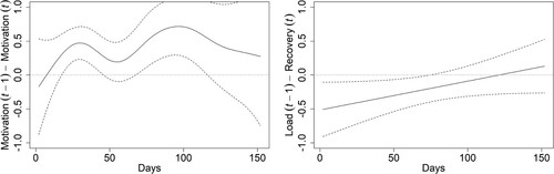
First, according to the model selection criteria, the BICs were calculated to check whether a time-invariant or time-varying model was a better model fit (see Table A1 for Player 1 and Table A2 for Player 2 in Appendix A). For player 1, the BIC scores indicated that all time-invariant models were better suited. For Player 2, the BIC scores of two models indicated a better model fit for the time-varying model. Subsequently, according to the next model selection criteria, all significant parameters of the superior model were selected (see Table A3 for Player 1 and Tables A4 and A5 for Player 2 in Appendix B). Since no time-varying model was selected for Player 1, we did not visually inspect the parameters for changes over time (model selection criteria (c)). In contrast, Player 2 revealed two models with time-varying parameters (Figure 1). In fact, the autoregressive effect of motivation displayed sinusoidal, that is nonlinear, changes over time. The sequence of change was as follows: small negative, to moderate positive, to small positive, to large positive, and back to small positive effect. In contrast, the changes in the cross-lagged effect of load on recovery were rather linear. The sequence of change was as follows: moderate negative to small positive effect. Hence, the visual inspection confirmed the presence of a time-varying effect in the two models.

Figure 1. The time-varying autoregressive effect of motivation (left) and the cross-lagged effect of recovery (right) of Player 2.

Note: The solid line shows the strength of the effect over time, whereas the dashed lines correspond to the 95% Bayesian Credible Intervals (i.e., the uncertainty of the smooth function). The horizontal line serves as guidance for an effect of 0. t–1 represents the previous point in time and t the current point in time.

As the last step, we translated the significant model parameters into interpretable network graphs for researchers and practitioners (Figure 2 for Player 1 and Figure 3 for Player 2). Note that the relations between determinants occur simultaneously and not in a step-by-step sequence. The results of Player 1 did not reveal any changing effects over time, meaning that the network of Player 1 did not change from early season to late season. In this network, self-efficacy appeared to play a central role, as it is the only key determinant predicting other factors. To be more specific, self-efficacy (before training/match) was predictive of distance, speed, heart rate (during training/match), and perceived performance and enjoyment (after training/match). This means that higher (lower) levels of self-efficacy experienced by Player 1, were followed by higher (lower) levels of other determinants at the next point in time (see section Practical Applications for some context of this finding). In addition, Player 1 showed positive autoregressive effects on self-efficacy, motivation, and perceived performance. Thus, when Player 1 experienced higher (lower) levels on these measures, the level of the same measure was also higher (lower) at the next point in time. Overall, the network density (or internode connectivity, i.e., the amount and strength of connections) was rather low with a total of eight edges, which were all positive. Therefore, changes in one determinant generally were not very predictive of other determinants.

Figure 2. Network graph of Player 1.

Note. The network remained stable across the season (i.e., no changes in effects). The green/solid edges represent positive effects and the thickness reflects the absolute value of the parameter estimate, that is, the magnitude of the effect (thicker edges display stronger effects and thinner edges display weaker effects). The self-loops show the autoregressive effects and the direct edges represent cross-lagged effects. We used NodeXL (https://nodexl.com/) with the Furchterman-Reingold layout to visualise the graphs.

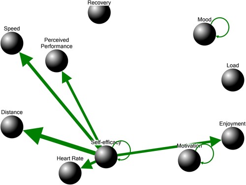
Figure 3. Network graph of Player 2.

Note. The network changed across the season. The green/solid edges represent positive effects, the red/dashed edges represent negative effects and the thickness reflects the absolute value of the parameter estimate, that is, the magnitude of the effect (thicker edges display stronger effects and thinner edges display weaker effects). The self-loops show the autoregressive effects and the direct edges represent cross-lagged effects. Changing effects (cf. Figure 1) are highlighted by a yellow/glowing shade around the edges. We used NodeXL (https://nodexl.com/) with the Furchterman-Reingold layout to visualise the graphs.

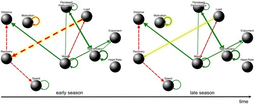
The results of Player 2 revealed changing effects in recovery and motivation over time. Accordingly, the network changed from early season to late season, which is visualised in the changing cross-lagged effect of load on recovery and the autoregressive effect of motivation. In contrast to Player 1, the network of Player 2 did not reveal one key determinant. In his network, every determinant (except for heart rate) was predictive of or predicted by, at least one other determinant or by itself. Overall, the network density was much higher, with a total of 16 edges, of which five (three in late season) were negative. This means that changes in one factor were more predictive of changes in other determinants and that the effect changed over time. Altogether, these results demonstrate the uniqueness of each player’s network structure by revealing information about the individual-specific temporal order of dynamic relationships between the key determinants of sports performance.⁶

Discussion

Within the scope of the present article, we argued that identifying the dynamic and individual-specific interactions of multidisciplinary key determinants of sports performance is an important avenue. To achieve this, we applied a recently developed analytical method (i.e., (TV)-VAR modelling). We specifically examined multiple psychological and physiological time series of two individual football players by analyzing their temporal order, and created network graphs to make the findings interpretable and useful for both researchers and practitioners.

First, our findings reveal that key determinants of performance dynamically evolve across a sports season. For instance, the motivation of both players displayed a spillover effect on itself over time. Only for Player 2, the magnitude of this effect changed over the course of the season, indicating a nonlinear data pattern. This emphasises the importance of examining time series rather than collecting data at one single, or only a few points in time (Den Hartigh et al., 2017; Salmon & McLean, 2020). Time series analyses will not only reveal if factors change over time but also when this happens (Bringmann et al., 2018). This may help coaches and sports psychologists to launch timely tailor-made interventions. For example, whereas the cross-lagged effect of load (measured at the end of the day) and recovery (measured the next morning) was negative at the beginning of the season for Player 2, it became weaker in the middle of the season, and eventually turned slightly positive at the end of the season. By recognising that this pattern arises in the data of an athlete, a coach could re-evaluate whether the training has yet the intended effect, and eventually adjust the training schedule. Interestingly, the positive spillover effect of motivation of the same player increased over the season. Previous research has shown that if the strength of autoregressive effects increases, humans may be less adaptive, need more time to recover, and stressors may have a stronger impact (Scheffer et al., 2018; Van De Leemput et al., 2014; Wichers & Groot, 2016). A coach or sports psychologist should closely observe this player and intervene when needed. Hence, the TV-VAR model could reveal information that would remain hidden when using the standard VAR, or any other statistical model based on stationarity.

Second, as expected, our results reveal unique network structures for both players, indicating that multidisciplinary key determinants of sports performance may behave in individual-specific ways. Although some effects were similar between Player 1 and Player 2 (e.g., the positive autoregressive effect of self-efficacy), the majority of relations, and therefore the overall network structures, differed. For instance, whereas for Player 2 the factor mood (measured at the beginning of the day) and the total distance covered (measured during training/match) showed a positive cross-lagged effect, we did not find such an effect for Player 1. Furthermore, self-efficacy played a central role for Player 1: It was the only factor that was predictive of other factors. In contrast, the network of Player 2 showed a greater distribution of relations between the different factors. Again, this emphasises the significance of a personalised approach in sports research and practice (Neumann et al., 2021; Robertson et al., 2017).

Third, we have demonstrated that multidisciplinary key determinants of sports performance are indeed interacting, which is in line with previous findings (Den Hartigh, Van Dijk, et al., 2016; Glazier, 2017). For instance, the level of mood of Player 2 was predictive of load, while at the same time, the level of load was predictive of mood. This means that key determinants of sports performance do not behave like a one-way street, but should rather be studied from a network perspective with variables that interact (and sometimes change) in individual-specific ways over time (Hill & Den Hartigh, 2023).

Strengths and limitations

This paper presents the first study in which multiple time series of nonexperimental sports field data have been analyzed with (TV-)VAR models, and next, have been visualised in network graphs. Whereas relations within and between performance determinants cannot be generalised across athletes as we have shown, the analysis methodology can be applied (i.e., generalised) across the population to provide individual-specific insights. However, some cautionary notes should also be acknowledged to properly apply the models. For instance, adding or removing variables from the analysis and gathering new data will most likely result in different outcomes. This study can thus be seen as a methods show-case, rather than a confirmatory analysis of relations between performance determinants that generalise to a group of people. However, this highlights our evidence-based assumption that performance determinants interact in individual-specific ways and may change over time (e.g., Den Hartigh et al., 2018; Neumann et al., 2021; Van der Sluis et al., 2019). Thus, when applying (TV-)VAR models, researchers and practitioners should select those factors that are relevant for the focus of their study (e.g., enhancing performance, decreasing the likelihood of injuries). When adding too many factors to the model, the probability of detecting false positives (i.e., spurious connections) increases. Regularisation techniques may serve as a valuable method for future research to reduce this issue and will likewise facilitate the interpretability of the models and networks for the practitioner (Bringmann et al., 2018).

Further, it should be noted that the models do not take into account measurement error, which may have an influence on the effects (Schuurman & Hamaker, 2018). However, measurement error hardly converges, which is also concluded by Schuurman and Hamaker (2018). Instead, innovations or dynamic errors are used in (TV-)VAR modelling, since they affect subsequent occasions as well due to the underlying dependencies in the process. Another important point relates to the sampling rate (i.e., how frequently one should measure). For our study, this sampling rate was appropriate, in the sense that we took a sufficient number of daily psychological and physiological measurements to capture the daily effects of trainings or matches. Other researchers aiming to apply the models should be aware that determining the optimal sampling rate is important to obtain reliable results (Adolf et al., 2021). However, even if the sampling rate is not optimal (e.g., too low), a strength of the (TV-)VAR models is that it smooths over the data to make it continuous and model the processes. Next to an appropriate sampling rate, the application of (TV)VAR models requires the data to be equidistant, meaning that measurements should take place at equally distant points in time (Haslbeck et al., 2020). For sports settings with high ecological validity, including the current context, meeting this requirement may be a challenge. For instance, football players do not practice every single day, their training is based on periodisation and is further adjusted due to unforeseen circumstances such as injuries (Kellmann et al., 2018). In any case, the data of the present study were approximately equidistant, which means that the distance between measurement points did not largely differ across time. In such cases, the application of (TV-)VAR models is possible, but researchers and practitioners should be aware that larger differences in measurement time intervals may mitigate the reliability of effects.

In addition, although (TV-)VAR models aim to capture how multiple factors are interconnected, they cannot entirely account for the complex behaviour of key performance determinants in sports. For instance, whereas the method can model gradual changes in the data, abrupt changes may also happen (Albers & Bringmann, 2020; Gernigon et al., 2010). Moreover, the models require defining a certain “lag” for the analysis (here “lag-1”) which does not account for multiple time scales (e.g., Carey et al., 2017; Hasselman, 2022). A final potential limitation in practice concerns the labour-intensiveness for longitudinal, daily data collection and manual data analysis. However, daily monitoring routines, advances in technology, and the automatic generation of network graphs make time series designs increasingly feasible (Bourdon et al., 2017; Emerencia et al., 2016; Van der Krieke et al., 2016). Effective and efficient implementations in the field ideally require a close collaboration between practitioners, psychologists, and data scientists (see Den Hartigh et al., 2022).

Practical implications and recommendations for future research

In this study, we have demonstrated that psychological and physiological time series data, collected on the sports field, can be meaningfully visualised through network graphs. By doing so, practitioners can be provided with interpretable insights into the individual-specific relations among key performance determinants. These insights may yield indicators for interventions at the individual level. For instance, self-efficacy of Player 1 turned out to be a key factor in his network. To be more specific, self-efficacy (measured at the beginning of the day) was predictive of perceived performance (measured at the end of the day) as well as the physiological factors distance, speed, and heart rate (measured during training/match). This indicates that every time the player experienced high levels of self-efficacy, the perceived and actual (e.g., distance, speed) performance was also high at the next point in time, which is in line with previous findings (Feltz & Lirgg, 2001; Moritz et al., 2000). Likewise, if the player experienced low levels of self-efficacy, the perceived and actual performance was also low at the next point in time, which might be a reason for coaches or sports psychologists to intervene, for instance, by specifically addressing the athlete’s self-efficacy (Feltz & Lirgg, 2001). Hence, the network graphs may serve as a monitoring device or decision-support system by providing indicators for which factors to intervene on, and when. Note, however, that intervening on one specific factor may result in changes in a diversity of factors since they are typically intertwined (Bringmann et al., 2019). In addition, network graphs can provide insights into the effectiveness of an intervention because the models show how the dynamics change over time (Haslbeck et al., 2020).

Future studies may apply (TV-)VAR models to study patterns in the networks of individual athletes, specifically in periods of performance gains and losses. For instance, researchers could focus on detecting and predicting Early Warning Signals (EWS). EWS represent instabilities in a system, which eventually lead to transitions between phases, such as from optimal performance to under-achievement (Hasselman, 2022; Hill et al., 2020; Hill & Den Hartigh, 2023; Scheffer et al., 2018; Wichers & Groot, 2016). To give an example, an increase in the cross-correlation (network density) may decrease an athlete’s resilience and possibly precede a performance loss. Identifying EWS enables practitioners to launch timely individual-specific interventions, aiming at facilitating a transition to a more optimal performance level or preventing performance losses in the first place.

Conclusion

In this paper, we show-cased that multidisciplinary key determinants of sports performance dynamically interact and change in individual-specific ways over time. More importantly, we add to the extant literature by providing the first empirical evidence that these dynamics can be adequately captured and explored with (TV-)VAR models. This innovative approach will yield new insights that may allow practitioners to develop effective, person-specific, targeted, and timely interventions. The presented study thereby offers a starting point to better understand the complex behaviour of key performance determinants within individual athletes.

Acknowledgments

The authors thank Dr Laura Bringmann for helpful and insightful comments and discussions regarding the analysis and Mees van der Linde for his support in collecting the data.

Disclosure statement

No potential conflict of interest was reported by the author(s).

Data availability statement

The R code has been made publicly available at DataVerseNL and can be accessed at https://dataverse.nl/privateurl.xhtml?token = eaf92882-1755-42df-86f5-d430f45b9dad [https://dataverse.nl/dataset.xhtml?persistentId=doi:10.34894/HNA8QQ]. The data contains sensitive information about the subjects and is therefore restricted from openly sharing it. Requests can be made by researchers affiliated with universities or independent, non-commercial research institutes via the same repository.

Additional information

Funding

This work was supported by The Netherlands Organization for Health Research and Development (ZonMw, grant number 546003004). The funding source had no role other than financial support.

Notes

1 Common approaches of dealing with nonstationarity are detrending or modelling the trend. This removes important information from the data and requires specifying the functional form of the trend. Time-varying modeling, however, detects trends in a data-driven way and does not require prespecifications to account for the trend (cf., Bringmann et al., 2017).

2 Reporting on a selected number of cases is common practice to demonstrate the merits of a methodology to better understand a process (e.g., Bringmann et al., 2018; Hasselman & Bosman, 2020; Wichers & Groot, 2016).

3 Here, we decided to pick an aggregate measure, but more specific measures could be possible as well. Examples are the Individualized Training Impulse (Manzi et al., 2009) and individualized speed zones (Palucci Vieira et al., 2019).

4 In order to retrieve interpretable results the process needs to be bounded, which is expressed as local stationarity (cf., Bringmann et al., 2018).

5 In contrast to other model selection criteria, such as the Akaike Information Criterion (AIC), the BIC is very conservative and strict because it tends to select a time-invariant model over a time-varying model to avoid overfitting, and therefore, false-positives (cf., Bringmann et al., 2018).

6 We performed the analysis on more players and we came to the same conclusion: Relations within and between determinants are individual-specific. Likewise, most relations remain stable while few change over time.

Appendices

Appendix A

Table A1. BIC Scores of the Time-Invariant and Time-Varying Models of Player 1.

Model (GAM)	Time-invariant	Time-varying
Recovery	299	312
Self-efficacy	281	295
Motivation	341	365
Mood	309	330
Distance	272	314
Speed	285	326
Heart Rate	290	315
Load	329	356
Perceived Performance	325	347
Enjoyment	335	371

Note. The better model fit is marked in bold.

Table A2. BIC Scores of the Time-Invariant and Time-Varying Models of Player 2.

Model (GAM)	Time-invariant	Time-varying
Recovery	363	361
Self-efficacy	291	310
Motivation	285	276
Mood	364	386
Distance	362	394
Speed	369	407
Heart Rate	365	402
Load	370	396
Perceived Performance	358	367
Enjoyment	367	411

Note. The better model fit is marked in bold.

Appendix B

Table A3. Significant Time-Invariant Parameters of Player 1

Model (GAM)	Parameter	Estimate	Std. Error	t	p
Self-efficacy	Self-efficacy	0.271	0.118	2.307	.023
Motivation	Motivation	0.282	0.127	2.217	.029
Mood	Mood	0.281	0.112	2.501	.014
Distance	Self-efficacy	0.793	0.174	4.569	<.001
Speed	Self-efficacy	0.570	0.189	3.024	.003
Heart Rate	Self-efficacy	0.457	0.187	2.444	.016
Perceived Performance	Self-efficacy	0.451	0.157	2.879	.005
Enjoyment	Self-efficacy	0.453	0.151	2.991	.003

Table A4. Significant Time-Invariant Parameters of Player 2.

Model (GAM)	Parameter	Estimate	Std. Error	t	p
Self-efficacy	Self-efficacy	0.439	0.071	6.212	<.001
	Perceived Performance	0.505	0.099	5.100	<.001
Mood	Mood	0.269	0.090	3.007	.003
	Load	−0.310	0.113	−2.735	.007
	Perceived Performance	0.243	0.123	1.983	.049
Distance	Recovery	−0.270	0.130	−2.078	.040
	Mood	0.398	0.105	3.807	<.001
Speed	Recovery	−0.291	0.133	−2.181	.031
	Speed	0.229	0.085	2.698	.008
Load	Mood	0.246	0.107	2.290	.024
Perceived Performance	Self-efficacy	0.260	0.114	2.276	.025
	Perceived Performance	0.248	0.106	2.342	.021
Enjoyment	Self-efficacy	0.233	0.111	2.094	.038
	Mood	0.294	0.107	2.756	.007

Table A5. Significant Time-Varying Parameters of Player 2.

Model (GAM)	Parameter	edf	F	p
Recovery	Load	2.000	3.453	.0353
Motivation	Motivation	6.175	4.727	<.001

Note. edf = effective degrees of freedom.

References

- Adolf, J. K., Loossens, T., Tuerlinckx, F., & Ceulemans, E. (2021). Optimal sampling rates for reliable continuous-time first-order autoregressive and vector autoregressive modeling. Psychological Methods, 26(6), 701–718. https://doi.org/10.1037/met0000398
- Akenhead, R., & Nassis, G. P. (2016). Training load and player monitoring in high-level football: Current practice and perceptions. International Journal of Sports Physiology and Performance, 11(5), 587–593. https://doi.org/10.1123/ijspp.2015-0331
- Albers, C. J., & Bringmann, L. F. (2020). Inspecting gradual and abrupt changes in emotion dynamics with the time-varying change point autoregressive model. European Journal of Psychological Assessment, 36(3), 492–499. https://doi.org/10.1027/1015-5759/a000589
- Bailey, C. (2019). Longitudinal monitoring of athletes: Statistical issues and best practices. Journal of Science in Sport and Exercise, 1(3), 217–227. https://doi.org/10.1007/s42978-019-00042-4
- Bandura, A. (2006). Guide for constructing self-efficacy scales. In T. Urdan, & F. Pajares (Eds.), Self-Efficacy beliefs of adolescents (pp. 307–337). Information Age Publishing.
- Barte, J. C. M., Nieuwenhuys, A., Geurts, S. A. E., & Kompier, M. A. J. (2019). Motivation counteracts fatigue-induced performance decrements in soccer passing performance. Journal of Sports Sciences, 37(10), 1189–1196. https://doi.org/10.1080/02640414.2018.1548919
- Bartlett, J. D., O’Connor, F., Pitchford, N., Torres-Ronda, L., & Robertson, S. J. (2017). Relationships between internal and external training load in team-sport athletes: Evidence for an individualized approach. International Journal of Sports Physiology and Performance, 12(2), 230–234. https://doi.org/10.1123/ijspp.2015-0791
- Birkhoff, B. D. (1931). Proof of the ergodic theorem. Proceedings of the National Academy of Sciences of the United States of America, 17(12), 656–660. https://doi.org/10.1073/pnas.17.2.656
- Blanchard, C. M., Mask, L., Vallerand, R. J., de la Sablonnière, R., & Provencher, P. (2007). Reciprocal relationships between contextual and situational motivation in a sport setting. Psychology of Sport and Exercise, 8(5), 854–873. https://doi.org/10.1016/j.psychsport.2007.03.004
- Borg, G. A. V. (1982). Psychophysical bases of perceived exertion. Medicine & Science in Sports & Exercise, 14(5), 377–381. https://doi.org/10.1249/00005768-198205000-00012
- Bourdon, P. C., Cardinale, M., Murray, A., Gastin, P., Kellmann, M., Varley, M. C., Gabbett, T. J., Coutts, A. J., Burgess, D. J., Gregson, W., & Cable, N. T. (2017). Monitoring athlete training loads: Consensus statement. International Journal of Sports Physiology and Performance, 12(s2), S2-161–S2-170. https://doi.org/10.1123/IJSPP.2017-0208
- Briki, W., Den Hartigh, R. J. R., Markman, K. D., Micallef, J. P., & Gernigon, C. (2013). How psychological momentum changes in athletes during a sport competition. Psychology of Sport and Exercise, 14(3), 389–396. https://doi.org/10.1016/j.psychsport.2012.11.009
- Bringmann, L. F., Elmer, T., Epskamp, S., Krause, R. W., Schoch, D., Wichers, M., Wigman, J., & Snippe, E. (2019). What do centrality measures measure in psychological networks? The Journal of Abnormal Psychology, 128(8), 12–19. https://doi.org/10.3929/ethz-a-010025751
- Bringmann, L. F., Ferrer, E., Hamaker, E. L., Borsboom, D., & Tuerlinckx, F. (2018). Modeling nonstationary emotion dynamics in dyads using a time-varying vector-autoregressive model. Multivariate Behavioral Research, 53(3), 293–314. https://doi.org/10.1080/00273171.2018.1439722
- Bringmann, L. F., Hamaker, E. L., Vigo, D. E., Aubert, A., Borsboom, D., & Tuerlinckx, F. (2017). Changing dynamics: Time-varying autoregressive models using generalized additive modeling. Psychological Methods, 22(3), 409–425. https://doi.org/10.1037/met0000085
- Bringmann, L. F., Pe, M. L., Vissers, N., Ceulemans, E., Borsboom, D., Vanpaemel, W., Tuerlinckx, F., & Kuppens, P. (2016). Assessing temporal emotion dynamics using networks. Assessment, 23(4), 425–435. https://doi.org/10.1177/1073191116645909
- Brink, M. S., Nederhof, E., Visscher, C., Schmikili, S. L., & Lemmink, K. A. P. M. (2010). Monitoring load, recovery, and performance in young elite soccer players. Journal of Strength and Conditioning Research, 24(3), 597–603. https://doi.org/10.1519/JSC.0b013e3181c4d38b
- Carey, D. L., Blanch, P., Ong, K. L., Crossley, K. M., Crow, J., & Morris, M. E. (2017). Training loads and injury risk in Australian football—differing acute: Chronic workload ratios influence match injury risk. British Journal of Sports Medicine, 51(16), 1215–1220. https://doi.org/10.1136/bjsports-2016-096309
- Cohen, A. B., Tenenbaum, G., & English, R. W. (2006). Emotions and golf performance: An IZOF-based applied sport psychology case study. Behavior Modification, 30(3), 259–280. https://doi.org/10.1177/0145445503261174
- Davids, K., Education, P., & Zealand, N. (2005). Applications of dynamical systems theory to football. In T. Reilly, J. Cabri, & D. Araújo (Eds.), Science and football V (pp. 570–572). Routledge. https://doi.org/10.4324/9780203412992-204
- Davids, K., Glazier, P., Araújo, D., & Bartlett, R. (2003). Movement systems as dynamical systems: The functional role of variability and its implications for sports medicine. Sports Medicine, 33(4), 245–260. https://doi.org/10.2165/00007256-200333040-00001
- Davids, K., Hristovski, R., Araújo, D., Serre, N. B., Button, C., & Passos, P. (2014). Complex systems in sport (1st ed.). Routledge.
- Den Hartigh, R. J. R., Gernigon, C., Van Yperen, N. W., Marin, L., & Van Geert, P. L. C. (2014). How psychological and behavioral team states change during positive and negative momentum. PLoS One, 9(5), e97887. https://doi.org/10.1371/journal.pone.0097887
- Den Hartigh, R. J. R., Hill, Y., & Van Geert, P. L. C. (2018). The development of talent in sports: A dynamic network approach. Complexity, 2018, 1–13. https://doi.org/10.1155/2018/9280154
- Den Hartigh, R. J. R., Meerhoff, L. R. A., Van Yperen, N. W., Neumann, N. D., Brauers, J. J., Frencken, W. G. P., Emerencia, A., Hill, Y., Platvoet, S., Atzmueller, M., Lemmink, K. A. P. M., & Brink, M. S. (2022). Resilience in sports: A multidisciplinary, dynamic, and personalized perspective. International Review of Sport and Exercise Psychology, 1–23. https://doi.org/10.1080/1750984X.2022.2039749
- Den Hartigh, R. J. R., Van Dijk, M. W. G., Steenbeek, H. W., & Van Geert, P. L. C. (2016). A dynamic network model to explain the development of excellent human performance. Frontiers in Psychology, 7, 532. https://doi.org/10.3389/fpsyg.2016.00532
- Den Hartigh, R. J. R., Van Geert, P. L. C., Van Yperen, N. W., Cox, R. F. A., & Gernigon, C. (2016). Psychological momentum during and across sports matches: Evidence for interconnected time scales. Journal of Sport and Exercise Psychology, 38(1), 82–92. https://doi.org/10.1123/jsep.2015-0162
- Den Hartigh, R. J. R., Van Yperen, N. W., & Van Geert, P. L. C. (2017). Embedding the psychosocial biographies of Olympic medalists in a (meta-)theoretical model of dynamic networks. In V. Walsh, M. Wilson, & B. Parkin (Eds.), Progress in brain research (1st ed., Vol. 232, pp. 137–140). Elsevier B.V. https://doi.org/10.1016/bs.pbr.2016.11.007
- Emerencia, A. C., Van Der Krieke, L., Bos, E. H., De Jonge, P., Petkov, N., & Aiello, M. (2016). Automating vector autoregression on electronic patient diary data. IEEE Journal of Biomedical and Health Informatics, 20(2), 631–643. https://doi.org/10.1109/JBHI.2015.2402280
- Feltz, D. L., & Lirgg, C. D. (2001). Self-efficacy beliefs of athletes, teams, and coaches. In R. N. Singer, H. A. Hausenblas, & C. Janelle (Eds.), Handbook of sport psychology (2nd ed., Vol. 2 (pp. 340–361). John Wiley and Sons.
- Fisher, A. J., Medaglia, J. D., & Jeronimus, B. F. (2018). Lack of group-to-individual generalizability is a threat to human subjects research. Proceedings of the National Academy of Sciences, 115(27), E6106–E6115. https://doi.org/10.1073/pnas.1711978115
- Fletcher, D., & Sarkar, M. (2012). A grounded theory of psychological resilience in Olympic champions. Psychology of Sport and Exercise, 13(5), 669–678. https://doi.org/10.1016/j.psychsport.2012.04.007
- Fortin-Guichard, D., Huberts, I., Sanders, J., van Elk, R., Mann, D. L., & Savelsbergh, G. J. P. (2022). Predictors of selection into an elite level youth football academy: A longitudinal study. Journal of Sports Sciences, 40(9), 984–999. https://doi.org/10.1080/02640414.2022.2044128
- Foster, C. (1998). Monitoring training in athletes with reference to overtraining syndrome. Medicine & Science in Sports & Exercise, 30(7), 1164–1168. https://doi.org/10.1097/00005768-199807000-00023
- Foster, C., Florhaug, J. A., Franklin, J., Gottschall, L., Hrovatin, L. A., Parker, S., Doleshal, P., & Dodge, C. (2001). A new approach to monitoring exercise training. Journal of Strenght and Conditioning Research, 15(1), 109–115. https://doi.org/10.1016/0968-0896(95)00066-P
- Gernigon, C., Briki, W., & Eykens, K. (2010). The dynamics of psychological momentum in sport: The role of ongoing history of performance patterns. Journal of Sport and Exercise Psychology, 32(3), 377–400. https://doi.org/10.1123/jsep.32.3.377
- Glazier, P. S. (2017). Towards a grand unified theory of sports performance. Human Movement Science, 56, 139–156. https://doi.org/10.1016/j.humov.2015.08.001
- Glazier, P. S., Davids, K., & Bartlett, R. (2003). Dynamical systems theory: A relevant framework for performance-oriented sports biomechanics research. Sportscience, 7, 1–8. http://www.sportsci.org/jour/03/psg.htm
- Haslbeck, J. M. B., Bringmann, L. F., & Waldorp, L. J. (2020). A tutorial on estimating time-varying vector autoregressive models. Multivariate Behavioral Research, 56(1), 120–149. https://doi.org/10.1080/00273171.2020.1743630
- Hasselman, F. (2022). Early warning signals in phase space: Geometric resilience loss indicators from multiplex cumulative recurrence networks. Frontiers in Physiology, 13, 859127. https://doi.org/10.3389/fphys.2022.859127
- Hasselman, F., & Bosman, A. M. T. (2020). Studying complex adaptive systems with internal states: A recurrence network approach to the analysis of multivariate time-series data representing self-reports of human experience. Frontiers in Applied Mathematics and Statistics, 6(9). https://doi.org/10.3389/fams.2020.00009
- Hill, Y., & Den Hartigh, R. J. R. (2023). Resilience in sports through the lens of dynamic network structures. Frontiers in Network Physiology, 3, 1190355. https://doi.org/10.3389/fnetp.2023.1190355
- Hill, Y., Den Hartigh, R. J. R., Cox, R. F. A., De Jonge, P., & Van Yperen, N. W. (2020). Predicting resilience losses in dyadic team performance. Nonlinear Dynamics, Psychology, and Life Sciences, 24(3), 327–351.
- Hill, Y., Den Hartigh, R. J. R., Meijer, R. R., De Jonge, P., & Van Yperen, N. W. (2018a). Resilience in sports from a dynamical perspective.. Sport, Exercise, and Performance Psychology, 7(4), 333–341. https://doi.org/10.1037/spy0000118
- Hill, Y., Den Hartigh, R. J. R., Meijer, R. R., De Jonge, P., & Van Yperen, N. W. (2018b). The temporal process of resilience.. Sport, Exercise, and Performance Psychology, 7(4), 363–370. https://doi.org/10.1037/spy0000143
- Hill, Y., Meijer, R. R., Van Yperen, N. W., Michelakis, G., Barisch, S., & Den Hartigh, R. J. R. (2021). Nonergodicity in protective factors of resilience in athletes.. Sport, Exercise, and Performance Psychology, 10(2), 217–223. https://doi.org/10.1037/spy0000246
- Jones, C. M., Griffiths, P. C., & Mellalieu, S. D. (2017). Training load and fatigue marker associations with injury and illness: A systematic review of longitudinal studies. Sports Medicine, 47(5), 943–974. https://doi.org/10.1007/s40279-016-0619-5
- Kellmann, M., Bertollo, M., Bosquet, L., Brink, M., Coutts, A. J., Duffield, R., Erlacher, D., Halson, S. L., Hecksteden, A., Heidari, J., Wolfgang Kallus, K., Meeusen, R., Mujika, I., Robazza, C., Skorski, S., Venter, R., & Beckmann, J. (2018). Recovery and performance in sport: Consensus statement. International Journal of Sports Physiology and Performance, 13(2), 240–245. https://doi.org/10.1123/ijspp.2017-0759
- Kenttä, G., & Hassmén, P. (1998). Overtraining and recovery. Sports Medicine, 26(1), 1–16. https://doi.org/10.2165/00007256-199826010-00001
- Lames, M., & McGarry, T. (2007). On the search for reliable performance indicators in game sports. International Journal of Performance Analysis in Sport, 7(1), 62–79. https://doi.org/10.1080/24748668.2007.11868388
- Mangalam, M., & Kelty-Stephen, D. G. (2021). Point estimates, simpson’s paradox, and nonergodicity in biological sciences. Neuroscience and Biobehavioral Reviews, 125, 98–107. https://doi.org/10.1016/j.neubiorev.2021.02.017
- Manzi, V., Iellamo, F., Impellizzeri, F., D’Ottavio, S., & Castagna, C. (2009). Relation between individualized training impulses and performance in distance runners. Medicine & Science in Sports & Exercise, 41(11), 2090–2096. https://doi.org/10.1249/MSS.0b013e3181a6a959
- Mara, J. K., Thompson, K. G., Pumpa, K. L., & Ball, N. B. (2015). Periodization and physical performance in elite female soccer players. International Journal of Sports Physiology and Performance, 10(5), 664–669. https://doi.org/10.1123/ijspp.2014-0345
- Moalla, W., Fessi, M. S., Farhat, F., Nouira, S., Wong, D. P., & Dupont, G. (2016). Relationship between daily training load and psychometric status of professional soccer players. Research in Sports Medicine, 24(4), 387–394. https://doi.org/10.1080/15438627.2016.1239579
- Molenaar, P. C. M., & Campbell, C. G. (2009). The new person-specific paradigm in psychology. Current Directions in Psychological Science, 18(2), 112–117. https://doi.org/10.1111/j.1467-8721.2009.01619.x
- Moritz, S. E., Feltz, D. L., Fahrbach, K. R., & Mack, D. E. (2000). The relation of self-efficacy measures to sport performance: A meta-analytic review. Research Quarterly for Exercise and Sport, 71(3), 280–294. https://doi.org/10.1080/02701367.2000.10608908
- Neumann, N. D., Van Yperen, N. W., Brauers, J. J., Frencken, W., Brink, M. S., Lemmink, K. A. M. P., Meerhoff, L. A., & Den Hartigh, R. J. R. (2021). Nonergodicity in load and recovery: Group results Do Not generalize to individuals. International Journal of Sports Physiology and Performance, 17(3), 391–399. https://doi.org/10.1123/ijspp.2021-0126
- Phillips, E., David, K., Renshaw, I., & Portus, M. (2010). Expert performance in sport and the dynamics of talend development. Sports Medicine, 40(4), 271–283. https://doi.org/10.2165/11319430-000000000-00000
- Puente-Díaz, R. (2012). The effect of achievement goals on enjoyment, effort, satisfaction and performance. International Journal of Psychology, 47(2), 102–110. https://doi.org/10.1080/00207594.2011.585159
- R Core Team. (2022). R: A language and environment for statistical computing (4.2.2.). R Foundation for Statistical Computing. http://www.r-project.org/.
- Robertson, S., Bartlett, J. D., & Gastin, P. B. (2017). Red, amber, or green? Athlete monitoring in team sport: The need for decision-support systems. International Journal of Sports Physiology and Performance, 12(s2), S2-73–S2-79. https://doi.org/10.1123/ijspp.2016-0541
- Rosmalen, J. G. M., Wenting, A. M. G., Roest, A. M., De Jonge, P., & Bos, E. H. (2012). Revealing causal heterogeneity using time series analysis of ambulatory assessments: Application to the association between depression and physical activity after myocardial infarction. Psychosomatic Medicine, 74(4), 377–386. https://doi.org/10.1097/PSY.0b013e3182545d47
- Salmon, P. M., & McLean, S. (2020). Complexity in the beautiful game: Implications for football research and practice. Science and Medicine in Football, 4(2), 162–167. https://doi.org/10.1080/24733938.2019.1699247
- Scheffer, M., Bolhuis, J. E., Borsboom, D., Buchman, T. G., Gijzel, S. M. W., Goulson, D., Kammenga, J. E., Kemp, B., van de Leemput, I. A., Levin, S., Martin, M. C., Melis, R. J. F., van Nes, E. H., Romero, L. M., & Olde Rikkert, M. G. M. (2018). Quantifying resilience of humans and other animals. Proceedings of the National Academy of Sciences of the United States of America, 115(47), 11883–11890. https://doi.org/10.1073/pnas.1810630115
- Schuurman, N. K., & Hamaker, E. L. (2018). Measurement error and person-specific reliability in multilevel. Psychological Methods, 24(1), 70–91. https://doi.org/10.1037/met0000188
- Stone, N. D. (1994). Overconfidence in initial self-efficacy judgments: Effects on decision processes and performance. Organizational Behavior and Human Decision Processes, 59(3), 452–474. https://doi.org/10.1006/obhd.1994.1069
- Thornton, H. R., Delaney, J. A., Duthie, G. M., & Dascombe, B. J. (2019). Developing athlete monitoring systems in team sports: Data analysis and visualization. International Journal of Sports Physiology and Performance, 14(6), 698–705. https://doi.org/10.1123/ijspp.2018-0169
- Totterdell, P. (2000). Catching moods and hitting runs: Mood linkage and subjective performance in professional sport teams. Journal of Applied Psychology, 85(6), 848–859. https://doi.org/10.1037/0021-9010.85.6.848
- Vancouver, J. B., Thompson, C. M., Tischner, E. C., & Putka, D. J. (2002). Two studies examining the negative effect of self-efficacy on performance. Journal of Applied Psychology, 87(3), 506–516. https://doi.org/10.1037/0021-9010.87.3.506
- Van De Leemput, I. A., Wichers, M., Cramer, A. O. J., Borsboom, D., Tuerlinckx, F., Kuppens, P., Van Nes, E. H., Viechtbauer, W., Giltay, E. J., Aggen, S. H., Derom, C., Jacobs, N., Kendler, K. S., Van Der Maas, H. L. J., Neale, M. C., Peeters, F., Thiery, E., Zachar, P., & Scheffer, M. (2014). Critical slowing down as early warning for the onset and termination of depression. Proceedings of the National Academy of Sciences of the United States of America, 111(1), 87–92. https://doi.org/10.1073/pnas.1312114110
- Van der Krieke, L., Blaauw, F. J., Emerencia, A. C., Schenk, H. M., Slaets, J. P. J., Bos, E. H., De Jonge, P., & Jeronimus, B. F. (2016a). Temporal dynamics of health and well-being: A crowdsourcing approach to momentary assessments and automated generation of personalized feedback. Psychosomatic Medicine, 79(2), 213–223. https://doi.org/10.1097/PSY.0000000000000378
- Van der Krieke, L., Jeronimus, B. F., Blaauw, F. J., Wanders, R. B. K., Emerencia, A. C., Schenk, H. M., Vos, S., Snippe, E., Wichers, M., Wigman, J. T. W., Bos, E. H., Wardenaar, K. J., & De Jonge, P. (2016b). Hownutsarethedutch (HoeGekIsNL): A crowdsourcing study of mental symptoms and strengths. International Journal of Methods in Psychiatric Research, 25(2), 123–144. https://doi.org/10.1002/mpr.1495
- Van der Sluis, J., Van der Steen, S., Stulp, G., & Den Hartigh, R. J. R. (2019). Visualizing individual dynamics: The case of a talented adolescent. In E. S. Kunnen, N. N. P. de Ruiter, B. F. Jeronimus, & M. A. E. van der Gaag (Eds.), Psychosocial development in adolescence: Insights from the dynamic systems approach (pp. 209–222). Routledge.
- Van Yperen, N. W., Jonker, L., & Verbeek, J. (2022). Predicting dropout from organized football: A prospective 4-year study Among adolescent and young adult football players. Frontiers in Sports and Active Living, 3, 752884. https://doi.org/10.3389/fspor.2021.752884
- Vieira, P., Carling, L. H., Barbieri, C., Aquino, F. A., & Santiago, R., & P, P. R. (2019). Match running performance in young soccer players: A systematic review. Sports Medicine, 49(2), 289–318. https://doi.org/10.1007/s40279-018-01048-8
- Wichers, M., & Groot, P. C. (2016). Critical slowing down as a personalized early warning signal for depression. Psychotherapy and Psychosomatics, 85(2), 114–116. https://doi.org/10.1159/000441458
- Williams, A. M., Ford, P. R., & Drust, B. (2020). Talent identification and development in soccer since the millennium. Journal of Sports Sciences, 38(11–12), 1199–1210. https://doi.org/10.1080/02640414.2020.1766647
- Wood, S. (2006). Generalized additive models: An introduction with R (1st ed.). Chapman and Hall/CRC. https://doi.org/10.1201/9781420010404
- Zentgraf, K., & Raab, M. (2023). Excellence and expert performance in sports: What do we know and where are we going? International Journal of Sport and Exercise Psychology, 21(5), 766–786. https://doi.org/10.1080/1612197X.2023.2229362