Kink, periodic and solitary solutions for coupled Benjamin–Bona–Mahony–KdV system

Abstract

In this paper, exp$(-\varphi (\tau ))$-expansion method, modified extended tanh-function method and Kudryashov method are used to investigate the exact solutions of the coupled Benjamin–Bona–Mahony–KdV (BBM-KdV) system. By the travelling wave transformation, the coupled BBM-KdV system is reduced to ordinary differential equations. Solving the nonlinear ordinary differential equations, kink, periodic and solitary solutions of the system are obtained. To further understand the natures of the solutions more intuitively, the dynamical behaviours of the solutions are given. The physical structures of the solutions are analysed in combination with 2D and 3D plots. These results enrich the available types of travelling wave solutions for the BBM-KdV model and are also useful for wave studies in complex engineering regions near the coast. It also proves the correctness and validity of our method.

Keywords:

• Coupled Benjamin–Bona–Mahony–KdV system
• travelling wave solutions exp$(-\varphi (\tau ))$-expansion method
• modified extended tanh-function method
• Kudryashov method

1. Introduction

In fluid mechanics, the Euler equations are a set of equations that control the motion of a viscosity-free fluid, which controls the surface waves of an ideal fluid under gravity. However, in practical researches and applications, most hydrodynamic equations, including the full Euler equation, are more complex than those needed for existing modelling, which limits the development of hydrodynamics to some extent. Many approximate models of Euler equations exist in literature, and one of the renowned system is Boussinesq system [1,2] given as (1) $\begin{array}{rl}& w_t+{\eta }_x+{\left(\mathrm{\eta w}\right)}_x+\mathcal{A}{\eta }_{\mathrm{xxx}}-B{w}_{\mathrm{xxt}}=0,\\ & {\eta }_t+w_x+\eta {\eta }_x+\mathcal{C}{w}_{\mathrm{xxx}}-\mathcal{D}{\eta }_{\mathrm{xxt}}=0,\end{array}$(1) in which w and η are unknown functions about x and t. In a channel of nearly constant depth χ there are small amplitude, long wavelength waves through uniformly, the conditions are expressed as (2) $\mu =\frac{\epsilon }{\chi }\ll 1,\nu =\frac{{\chi }^2}{l^2}\ll 1,R=\frac{\mu }{\nu }=\frac{\epsilon l^2}{{\chi }^3}\approx 1,$(2) in which ε is the wave amplitude and l is the wavelength. Equation (1(1) $\begin{array}{rl}& w_t+{\eta }_x+{\left(\mathrm{\eta w}\right)}_x+\mathcal{A}{\eta }_{\mathrm{xxx}}-B{w}_{\mathrm{xxt}}=0,\\ & {\eta }_t+w_x+\eta {\eta }_x+\mathcal{C}{w}_{\mathrm{xxx}}-\mathcal{D}{\eta }_{\mathrm{xxt}}=0,\end{array}$(1) ) are first-order approximations (in µ and ν of (2(2) $\mu =\frac{\epsilon }{\chi }\ll 1,\nu =\frac{{\chi }^2}{l^2}\ll 1,R=\frac{\mu }{\nu }=\frac{\epsilon l^2}{{\chi }^3}\approx 1,$(2) )) to the Euler equations. The system (1(1) $\begin{array}{rl}& w_t+{\eta }_x+{\left(\mathrm{\eta w}\right)}_x+\mathcal{A}{\eta }_{\mathrm{xxx}}-B{w}_{\mathrm{xxt}}=0,\\ & {\eta }_t+w_x+\eta {\eta }_x+\mathcal{C}{w}_{\mathrm{xxx}}-\mathcal{D}{\eta }_{\mathrm{xxt}}=0,\end{array}$(1) ) describes the two-way propagation of long gravity waves over the water surface of the channel, and it can also simulate the propagation of long peaked waves in the marine environment. The $\mathcal{A}$, $\mathcal{B}$, $\mathcal{C}$, $\mathcal{D}$ in the system (1(1) $\begin{array}{rl}& w_t+{\eta }_x+{\left(\mathrm{\eta w}\right)}_x+\mathcal{A}{\eta }_{\mathrm{xxx}}-B{w}_{\mathrm{xxt}}=0,\\ & {\eta }_t+w_x+\eta {\eta }_x+\mathcal{C}{w}_{\mathrm{xxx}}-\mathcal{D}{\eta }_{\mathrm{xxt}}=0,\end{array}$(1) ) are defined by the parameters ℏ, κ and θ $(0<\theta <1)$ as follows (3) $\begin{array}{rl}\mathcal{A}& =\frac{1}{2}\left({\theta }^2-\frac{1}{3}\right)\hslash ,\mathcal{B}=\frac{1}{2}\left({\theta }^2-\frac{1}{3}\right)\left(1-\hslash \right),\\ \mathcal{C}& =\frac{1}{2}\left(1-{\theta }^2\right)\kappa ,\mathcal{D}=\frac{1}{2}\left(1-{\theta }^2\right)\left(1-\kappa \right).\end{array}$(3) When ℏ, κ, θ take different values, many models with physical meaning can be obtained. For example, when $\hslash =0$, $\kappa =0$, ${\theta }^2=\frac{2}{3}$, the coupled Benjamin–Bona–Mahony (BBM) system is derived, in [3–5], the numerical and travelling wave solutions of this system are studied, and Wu et al. considered numerical solutions of this system in 1D and 2D utilizing the Galerkin finite element method [6]. The Bona-Smith (BS) system is obtained when $\hslash =0$, $\kappa <0$, ${\theta }^2=\frac{(\frac{4}{3}-\kappa )}{2-\kappa }$, Dougalis and Mitsotakis investigated and analysed the solutions of the BS system [7,8]; When $\hslash =0$, $\kappa =1$, ${\theta }^2=\frac{2}{3}$, the system (1(1) $\begin{array}{rl}& w_t+{\eta }_x+{\left(\mathrm{\eta w}\right)}_x+\mathcal{A}{\eta }_{\mathrm{xxx}}-B{w}_{\mathrm{xxt}}=0,\\ & {\eta }_t+w_x+\eta {\eta }_x+\mathcal{C}{w}_{\mathrm{xxx}}-\mathcal{D}{\eta }_{\mathrm{xxt}}=0,\end{array}$(1) ) can be simplified to the coupled BBM-KdV system (4) $\begin{array}{rl}& w_t+{\eta }_x+{\left(\mathrm{w\eta }\right)}_x-\frac{1}{6}{w}_{\mathrm{xxt}}=0,\\ & {\eta }_t+w_x+\eta {\eta }_x+\frac{1}{6}{w}_{\mathrm{xxx}}=0,\end{array}$(4) which is an essential model for the unidirectional propagation of long waves in weakly nonlinear dispersive media. The model is valuable for the design of harbour piers, breakwaters and other buildings, as well as the calculation of the evolution of the near-shore seabe and other offshore projects.

It is worth noticing that nonlinear partial differential equations (NLPDEs) [9–11], including Equation (4(4) $\begin{array}{rl}& w_t+{\eta }_x+{\left(\mathrm{w\eta }\right)}_x-\frac{1}{6}{w}_{\mathrm{xxt}}=0,\\ & {\eta }_t+w_x+\eta {\eta }_x+\frac{1}{6}{w}_{\mathrm{xxx}}=0,\end{array}$(4) ), are important in the fields of hydrodynamics, oceanography and physics, so solving the exact solutions of NLPDEs is particularly important. At present, many methods for solving the NLPDEs were established, such as: Lie symmetry analysis method [12], dynamical system method [13–15],ansatz function method [16–19], Reiman-Hilbert method [20], extended trial equation method [21–23], bilinear method [24–26], exponential rational function method [27], variational method [28,29] and so on [30–36]. Constructing exact solutions of equations from a quantitative point of view has been a hot research topic, in recent years a number of new construction methods have been presented, for example, Sardar subequation method [37], Wang's direct mapping method [38,39]. However, these methods are not all-powerful. There is no one method that can solve all NLPDEs. And some methods are tedious in dealing with NLPDEs. So we need to seek suitable and easy to compute methods to solve the system (4(4) $\begin{array}{rl}& w_t+{\eta }_x+{\left(\mathrm{w\eta }\right)}_x-\frac{1}{6}{w}_{\mathrm{xxt}}=0,\\ & {\eta }_t+w_x+\eta {\eta }_x+\frac{1}{6}{w}_{\mathrm{xxx}}=0,\end{array}$(4) ).

The exp$(-\varphi (\tau ))$ – expansion method [40–42], the modified extended tanh-function method [43] and Kudryashov method [44] are used by a wide range of scholars to study the exact solutions of NLPDEs. Among them, the Kudryashov method can directly build a category of soliton solutions of NLODEs. Bashar applied the exp$(-\varphi (\tau ))$ – expansion method to fractional modified Kawahara equation [45]. Alam used the modified extended tanh-function method to study the travelling wave solution of the fractional CBS equation [46]. Hubert investigated soliton solutions in nonlinear transport employing the Kudryashov method [47]. These studies show that the above three methods are very effective for solving NLPDEs. Currently, there are no relevant works on applying these methods mentioned above to solve the travelling wave solution of Equation (4(4) $\begin{array}{rl}& w_t+{\eta }_x+{\left(\mathrm{w\eta }\right)}_x-\frac{1}{6}{w}_{\mathrm{xxt}}=0,\\ & {\eta }_t+w_x+\eta {\eta }_x+\frac{1}{6}{w}_{\mathrm{xxx}}=0,\end{array}$(4) ), yet these methods are straightforward and easy to handle. As such, in this paper, the three methods mentioned above are used to study the exact travelling wave solution of the system (4(4) $\begin{array}{rl}& w_t+{\eta }_x+{\left(\mathrm{w\eta }\right)}_x-\frac{1}{6}{w}_{\mathrm{xxt}}=0,\\ & {\eta }_t+w_x+\eta {\eta }_x+\frac{1}{6}{w}_{\mathrm{xxx}}=0,\end{array}$(4) ).

The structure of this paper is as follows: In Section 2, describes the exp$(-\varphi (\tau ))$ - expansion method, the modified extended tanh-function method and Kudryashov method in detail. In Section 3, the three methods mentioned above are applied to Equation (4(4) $\begin{array}{rl}& w_t+{\eta }_x+{\left(\mathrm{w\eta }\right)}_x-\frac{1}{6}{w}_{\mathrm{xxt}}=0,\\ & {\eta }_t+w_x+\eta {\eta }_x+\frac{1}{6}{w}_{\mathrm{xxx}}=0,\end{array}$(4) ), and the kink solutions, solitary solutions and periodic blast solutions of Equation (4(4) $\begin{array}{rl}& w_t+{\eta }_x+{\left(\mathrm{w\eta }\right)}_x-\frac{1}{6}{w}_{\mathrm{xxt}}=0,\\ & {\eta }_t+w_x+\eta {\eta }_x+\frac{1}{6}{w}_{\mathrm{xxx}}=0,\end{array}$(4) ) are obtained, while plots of dynamical behaviours of the corresponding solutions are drawn. In Section 4, the physical structures of the acquired solutions are discussed in detail, as well as the results of this paper are contrasted with the available results.

2. Description of three methods

In this part, we present the descriptions of exp$(-\varphi (\tau ))$ – expansion method, the modified extended tanh-function method and Kudryashov method step wise.

Considering the following NLPDEs (5) $\mathcal{G}(w,w_x,w_t,w_{\mathrm{xx}},w_{\mathrm{tt}},\dots )=0,$(5) introducing the travelling wave transform (6) $w(x,t)=w(\tau ),\tau =x-\mathrm{ct},$(6) in which c>0 is an arbitrary constant. Substituting (6(6) $w(x,t)=w(\tau ),\tau =x-\mathrm{ct},$(6) ) into Equation (5(5) $\mathcal{G}(w,w_x,w_t,w_{\mathrm{xx}},w_{\mathrm{tt}},\dots )=0,$(5) ) yields an ordinary differential equation (ODEs) (7) $\mathcal{F}(w,w^{\prime },w^{″},\dots )=0,$(7) where $w^{\prime }=\frac{d}{\mathrm{d\tau }}$.

2.1. exp$(-\varphi (\tau ))$ – expansion method

Assuming that Equation (7(7) $\mathcal{F}(w,w^{\prime },w^{″},\dots )=0,$(7) ) has solutions of the following exp$(-\varphi (\tau ))$ form (8) $\begin{array}{rl}w(\xi )& =a_j(\exp (-\varphi (\tau )){)}^j\\ & +a_{j-1}(\exp (-\varphi (\tau )){)}^{j-1}+\cdots ,a_j\ne 0,\end{array}$(8) where ${\varphi }^{\prime }(\tau )=\frac{\mathrm{d\varphi }(\tau )}{\mathrm{d\tau }}$ satisfies (9) ${\varphi }^{\prime }(\tau )=\exp (-\varphi (\tau ))+\mathrm{\kappa exp}(\varphi (\tau ))+\hslash .$(9) The solutions for Equation (9(9) ${\varphi }^{\prime }(\tau )=\exp (-\varphi (\tau ))+\mathrm{\kappa exp}(\varphi (\tau ))+\hslash .$(9) ) have the following five cases

1. When ${\hslash }^2-4\kappa >0$, $\kappa \ne 0$, $\varphi (\tau )=\ln (\frac{-\sqrt{{\hslash }^2-4\kappa }\tanh (\frac{\sqrt{{\hslash }^2-4\kappa }}{2}(\tau +c_1))-\hslash }{2\kappa })$;

2. When ${\hslash }^2-4\kappa >0$, $\kappa =0$, $\varphi (\tau )=-\ln (\frac{\hslash }{\exp (\hslash (\tau +c_1))-1})$;

3. When ${\hslash }^2-4\kappa =0$, $\hslash \ne 0$, $\kappa \ne 0$, $\varphi (\tau )=\ln (-\frac{2(\hslash (\tau +c_1)+2)}{{\hslash }^2(\tau +c_1)})$;

4. When ${\hslash }^2-4\kappa =0$, $\hslash =0$, $\kappa =0$, $\varphi (\tau )=\ln (\tau +c_1)$;

5. When ${\hslash }^2-4\kappa <0$, $\varphi (\tau )=\ln (\frac{\sqrt{4\kappa -{\hslash }^2}\tan (\frac{\sqrt{4\kappa -{\hslash }^2}}{2}(\tau +c_1))-\hslash }{2\kappa })$, in which $c_1$ is an arbitrary constant and $a_j$, ···  ℏ, κ are the constants to be determined.

Then, substituting (8(8) $\begin{array}{rl}w(\xi )& =a_j(\exp (-\varphi (\tau )){)}^j\\ & +a_{j-1}(\exp (-\varphi (\tau )){)}^{j-1}+\cdots ,a_j\ne 0,\end{array}$(8) ) into Equation (7(7) $\mathcal{F}(w,w^{\prime },w^{″},\dots )=0,$(7) ), according to (9(9) ${\varphi }^{\prime }(\tau )=\exp (-\varphi (\tau ))+\mathrm{\kappa exp}(\varphi (\tau ))+\hslash .$(9) ), collecting the coefficients of $\exp (-\mathrm{n\varphi }(\tau ))$ and letting each the coefficients be zero, so as to find $a_j$, ··· , ℏ, κ.

Finally, by substituting the resulting solution $\varphi (\tau )$ into (8(8) $\begin{array}{rl}w(\xi )& =a_j(\exp (-\varphi (\tau )){)}^j\\ & +a_{j-1}(\exp (-\varphi (\tau )){)}^{j-1}+\cdots ,a_j\ne 0,\end{array}$(8) ), the travelling wave solutions of Equation (7(7) $\mathcal{F}(w,w^{\prime },w^{″},\dots )=0,$(7) ) are got.

2.2. Modified extended tanh-function method

Assuming Equation (7(7) $\mathcal{F}(w,w^{\prime },w^{″},\dots )=0,$(7) ) has solutions of the following form for σ : (10) $w(\tau )=\sum _{i=0}^n\left(a_i{\sigma }^i+b_i{\sigma }^{-i}\right),$(10) in which $a_i$, $b_i$ are constants to be determined later and n is the balancing number. In Equation (10(10) $w(\tau )=\sum _{i=0}^n\left(a_i{\sigma }^i+b_i{\sigma }^{-i}\right),$(10) ), σ satisfies the Riccati function (11) ${\sigma }^{\prime }=\delta +{\sigma }^2,$(11) in which δ is a constant and the solutions of Equation (11(11) ${\sigma }^{\prime }=\delta +{\sigma }^2,$(11) ) has the following three cases

1. When $\delta <0$, then $\sigma =-\sqrt{-\delta }\tanh (\sqrt{-\delta }\tau )$, or $\sigma =-\sqrt{-\delta }\coth (\sqrt{-\delta }\tau )$;

2. When $\delta >0$, then $\sigma =\sqrt{\delta }\tan (\sqrt{\delta }\tau )$, or $\sigma =-\sqrt{\delta }\cot (\sqrt{\delta }\tau )$;

3. When $\delta =0$, then $\sigma =-\frac{1}{\tau }$.

Substituting Equations (10(10) $w(\tau )=\sum _{i=0}^n\left(a_i{\sigma }^i+b_i{\sigma }^{-i}\right),$(10) ) and (11(11) ${\sigma }^{\prime }=\delta +{\sigma }^2,$(11) ) into Equation (7(7) $\mathcal{F}(w,w^{\prime },w^{″},\dots )=0,$(7) ), the polynomial in ${\sigma }^i$ $(i=0,\pm 1,\pm 2,\dots )$ are obtained. Let all the coefficients equal to zero, we acquire a set of over determined nonlinear algebraic equations. By solving these equations, the travelling wave solutions of Equation (5(5) $\mathcal{G}(w,w_x,w_t,w_{\mathrm{xx}},w_{\mathrm{tt}},\dots )=0,$(5) ) are found out.

2.3. Kudryashov method

The exact solutions of Equation (7(7) $\mathcal{F}(w,w^{\prime },w^{″},\dots )=0,$(7) ) are found by means of following form (12) $w(\tau )=\sum _{i=0}^n{a}_i{\left[S\left(\tau \right)\right]}^i,$(12) in which $a_i$ are the uncertain constants to be investigated subsequently, while $S(\tau )$ takes the following functional form (13) $S\left(\tau \right)=\frac{1}{1+e^{\tau }},$(13) and $S(\tau )$ satisfies (14) $\frac{\mathrm{dS}\left(\tau \right)}{\mathrm{d\tau }}=S^2\left(\tau \right)-S\left(\tau \right).$(14) Then, considering the necessary derivatives of $w(\tau )$, the necessary derivatives, (12(12) $w(\tau )=\sum _{i=0}^n{a}_i{\left[S\left(\tau \right)\right]}^i,$(12) ) and (13(13) $S\left(\tau \right)=\frac{1}{1+e^{\tau }},$(13) ) are substituted into Equation (7(7) $\mathcal{F}(w,w^{\prime },w^{″},\dots )=0,$(7) ). By collecting polynomials of the same $S^i(\tau )$ and making them zero, a set of equations is obtained. Solving this set of equations with the help of maple software yields $a_i$.

3. Application of the methods to the BBM-KdV system

In this section, the exp$(-\varphi (\tau ))$-expansion method, the modified extended tanh-function method and Kudryashov method are applied to the BBM-KdV system to get the kink, periodic, solitary solutions of system (4(4) $\begin{array}{rl}& w_t+{\eta }_x+{\left(\mathrm{w\eta }\right)}_x-\frac{1}{6}{w}_{\mathrm{xxt}}=0,\\ & {\eta }_t+w_x+\eta {\eta }_x+\frac{1}{6}{w}_{\mathrm{xxx}}=0,\end{array}$(4) ) and the dynamical behaviours of these solutions are plotted.

Considering the BBM-KdV syetem (4(4) $\begin{array}{rl}& w_t+{\eta }_x+{\left(\mathrm{w\eta }\right)}_x-\frac{1}{6}{w}_{\mathrm{xxt}}=0,\\ & {\eta }_t+w_x+\eta {\eta }_x+\frac{1}{6}{w}_{\mathrm{xxx}}=0,\end{array}$(4) ), by the wave transformation $\tau =x-\mathrm{ct}$, system (4(4) $\begin{array}{rl}& w_t+{\eta }_x+{\left(\mathrm{w\eta }\right)}_x-\frac{1}{6}{w}_{\mathrm{xxt}}=0,\\ & {\eta }_t+w_x+\eta {\eta }_x+\frac{1}{6}{w}_{\mathrm{xxx}}=0,\end{array}$(4) ) reduces to the following system (15) $\begin{array}{rl}-c{w}^{\prime }+{\eta }^{\prime }+(\mathrm{w\eta }{)}^{\prime }+\frac{c}{6}{w}^{‴}& =0,\\ -c{\eta }^{\prime }+w^{\prime }+\eta {\eta }^{\prime }+\frac{1}{6}{w}^{‴}& =0.\end{array}$(15)

3.1. Application of exp$(\mathbf{-}\varphi \mathbf{(}\tau \mathbf{)})$ – expansion method to Equation (4)

To solve the Equation (15(15) $\begin{array}{rl}-c{w}^{\prime }+{\eta }^{\prime }+(\mathrm{w\eta }{)}^{\prime }+\frac{c}{6}{w}^{‴}& =0,\\ -c{\eta }^{\prime }+w^{\prime }+\eta {\eta }^{\prime }+\frac{1}{6}{w}^{‴}& =0.\end{array}$(15) ), integrating Equation (15(15) $\begin{array}{rl}-c{w}^{\prime }+{\eta }^{\prime }+(\mathrm{w\eta }{)}^{\prime }+\frac{c}{6}{w}^{‴}& =0,\\ -c{\eta }^{\prime }+w^{\prime }+\eta {\eta }^{\prime }+\frac{1}{6}{w}^{‴}& =0.\end{array}$(15) ) yields (16) $\eta =\frac{2}{c}(w+1).$(16) Substituting (16(16) $\eta =\frac{2}{c}(w+1).$(16) ) into system (15(15) $\begin{array}{rl}-c{w}^{\prime }+{\eta }^{\prime }+(\mathrm{w\eta }{)}^{\prime }+\frac{c}{6}{w}^{‴}& =0,\\ -c{\eta }^{\prime }+w^{\prime }+\eta {\eta }^{\prime }+\frac{1}{6}{w}^{‴}& =0.\end{array}$(15) ) yields (17) $(\frac{4}{c}-c)w^{\prime }+\frac{4}{c}w{w}^{\prime }+\frac{c}{6}{w}^{‴}=0.$(17) Balancing $w^{‴}$ and $w{w}^{\prime }$ in Equation (17(17) $(\frac{4}{c}-c)w^{\prime }+\frac{4}{c}w{w}^{\prime }+\frac{c}{6}{w}^{‴}=0.$(17) ), we get n + 1 + n = n + 3 ⇒ n = 2. Therefore, according to (8(8) $\begin{array}{rl}w(\xi )& =a_j(\exp (-\varphi (\tau )){)}^j\\ & +a_{j-1}(\exp (-\varphi (\tau )){)}^{j-1}+\cdots ,a_j\ne 0,\end{array}$(8) ), we obtain (18) $w(\tau )=a_0+a_1\exp (-\varphi (\tau ))+a_2\exp (-\varphi (\tau ){)}^2.$(18) Then, substituting (18(18) $w(\tau )=a_0+a_1\exp (-\varphi (\tau ))+a_2\exp (-\varphi (\tau ){)}^2.$(18) ) into Equation (17(17) $(\frac{4}{c}-c)w^{\prime }+\frac{4}{c}w{w}^{\prime }+\frac{c}{6}{w}^{‴}=0.$(17) ). The coefficients of exp$(-\varphi (\tau ))$ are collected and made to be zero, we acquire the following equations (19) $\begin{array}{rl}& -\frac{1}{c}\left(4a_2{c}^2+8{a_2}^2\right)=0,\\ & -\frac{1}{c}\left(9a_2{c}^2\hslash +a_1{c}^2+8{a_2}^2\hslash +12a_1{a}_2\right)=0,\\ & -\frac{1}{6c}(40a_2{c}^2\kappa +38a_2{c}^2{\hslash }^2+48{a_2}^2\kappa \\ & +12a_1{c}^2\hslash +72a_1{a}_2\hslash -12a_2{c}^2+48a_0{a}_2\\ & +24{a_1}^2+48a_2)=0,\\ & -\frac{1}{6c}(52a_2{c}^2\mathrm{\hslash \kappa }+8a_1{c}^2\kappa +72a_1{a}_2\kappa \\ & +8a_2{c}^2{\hslash }^3+7a_1{c}^2{\hslash }^2-12a_2{c}^2\hslash \\ & +48a_0{a}_2\hslash +24{a_1}^2\hslash \\ & -6a_1{c}^2+24a_0{a}_1+48a_2\hslash +24a_1)=0,\\ & -\frac{8}{3}{a}_{2}c{\kappa }^2-\frac{1}{6c}(14a_2{c}^2{\hslash }^2\kappa +8a_1{c}^2\mathrm{\hslash \kappa }-12a_2{c}^2\kappa \\ & +48a_0{a}_2\kappa +24{a_1}^2\kappa +48a_2\kappa +a_1{c}^2{\hslash }^3\\ & -6a_1{c}^2\hslash +24a_0{a}_1\hslash +24a_1)=0,\\ & -\frac{1}{6c}(6a_2{c}^2\hslash {\beta }^2+2a_1{c}^2{\kappa }^2+a_1{c}^2{\hslash }^2\kappa -6a_1{c}^2\kappa \\ & +24a_0{a}_1\kappa +24a_1\kappa )=0.\end{array}$(19) Solving for Equation (19(19) $\begin{array}{rl}& -\frac{1}{c}\left(4a_2{c}^2+8{a_2}^2\right)=0,\\ & -\frac{1}{c}\left(9a_2{c}^2\hslash +a_1{c}^2+8{a_2}^2\hslash +12a_1{a}_2\right)=0,\\ & -\frac{1}{6c}(40a_2{c}^2\kappa +38a_2{c}^2{\hslash }^2+48{a_2}^2\kappa \\ & +12a_1{c}^2\hslash +72a_1{a}_2\hslash -12a_2{c}^2+48a_0{a}_2\\ & +24{a_1}^2+48a_2)=0,\\ & -\frac{1}{6c}(52a_2{c}^2\mathrm{\hslash \kappa }+8a_1{c}^2\kappa +72a_1{a}_2\kappa \\ & +8a_2{c}^2{\hslash }^3+7a_1{c}^2{\hslash }^2-12a_2{c}^2\hslash \\ & +48a_0{a}_2\hslash +24{a_1}^2\hslash \\ & -6a_1{c}^2+24a_0{a}_1+48a_2\hslash +24a_1)=0,\\ & -\frac{8}{3}{a}_{2}c{\kappa }^2-\frac{1}{6c}(14a_2{c}^2{\hslash }^2\kappa +8a_1{c}^2\mathrm{\hslash \kappa }-12a_2{c}^2\kappa \\ & +48a_0{a}_2\kappa +24{a_1}^2\kappa +48a_2\kappa +a_1{c}^2{\hslash }^3\\ & -6a_1{c}^2\hslash +24a_0{a}_1\hslash +24a_1)=0,\\ & -\frac{1}{6c}(6a_2{c}^2\hslash {\beta }^2+2a_1{c}^2{\kappa }^2+a_1{c}^2{\hslash }^2\kappa -6a_1{c}^2\kappa \\ & +24a_0{a}_1\kappa +24a_1\kappa )=0.\end{array}$(19) ), we have (20) $\begin{array}{rl}{a}_0& =-\frac{1}{24}{c}^2{\kappa }^2-\frac{1}{3}{c}^2\kappa +\frac{1}{4}{c}^2-1,a_1=-\frac{1}{2}{c}^2\hslash ,\\ a_2& =-\frac{1}{2}{c}^2,\hslash =\hslash ,\kappa =\kappa .\end{array}$(20) Consequently, the solutions of the following cases are obtained

$\mathbf{Case}\mathbf{I}$. If ${\hslash }^2-4\kappa >0$, $\kappa \ne 0$, (21) $\begin{array}{rl}& w\left(\tau \right)\\ & =-\frac{1}{24}{c}^2{\hslash }^2-\frac{1}{3}{c}^2\kappa +\frac{1}{4}{c}^2-1\\ & -\left(\frac{c^2\mathrm{\hslash \kappa }}{-\sqrt{{\hslash }^2-4\kappa }\tanh \left(\frac{\sqrt{{\hslash }^2-4\kappa }}{2}\left(\tau +c_1\right)\right)-\hslash }\right)\\ & -\frac{1}{2}\left(\frac{c^6{\hslash }^2{\kappa }^2}{{\left(-\sqrt{{\hslash }^2-4\kappa }\tanh \left(\frac{\sqrt{{\hslash }^2-4\kappa }}{2}\left(\tau +c_1\right)\right)-\hslash \right)}^2}\right),\end{array}$(21) (22) $\begin{array}{rl}& \eta \left(\tau \right)\\ & =-\frac{1}{12}c{\hslash }^2-\frac{2}{3}c\kappa +\frac{1}{2}c\\ & -\left(\frac{2c\mathrm{\hslash \kappa }}{-\sqrt{{\hslash }^2-4\kappa }\tanh \left(\frac{\sqrt{{\hslash }^2-4\kappa }}{2}\left(\tau +c_1\right)\right)-\hslash }\right)\\ & -\left(\frac{c^5{\hslash }^2{\kappa }^2}{{\left(-\sqrt{{\hslash }^2-4\kappa }\tanh \left(\frac{\sqrt{{\hslash }^2-4\kappa }}{2}\left(\tau +c_1\right)\right)-\hslash \right)}^2}\right).\end{array}$(22)

$\mathbf{Case}\mathbf{II}$. If ${\hslash }^2-4\kappa >0$, $\kappa =0$, (23) $\begin{array}{rl}w\left(\tau \right)& =-\frac{1}{24}{c}^2{\hslash }^2-\frac{1}{3}{c}^2\kappa +\frac{1}{4}{c}^2-1\\ & -\frac{a_1\hslash }{2\left(\exp \left(\hslash \left(\tau +c_1\right)\right)-1\right)}\\ & -\frac{c^6{\hslash }^4}{8{\left(\exp \left(\hslash \left(\tau +c_1\right)\right)-1\right)}^2},\end{array}$(23) (24) $\begin{array}{rl}\eta \left(\tau \right)& =-\frac{1}{12}c{\hslash }^2-\frac{2}{3}c\kappa +\frac{1}{2}c\\ & -\frac{a_1\hslash }{c\left(\exp \left(\hslash \left(\tau +c_1\right)\right)-1\right)}\\ & -\frac{c^5{\hslash }^4}{4{\left(\exp \left(\hslash \left(\tau +c_1\right)\right)-1\right)}^2}.\end{array}$(24)

$\mathbf{Case}\mathbf{III}$. If ${\hslash }^2-4\kappa =0$, $\hslash \ne 0$, $\kappa \ne 0$, (25) $\begin{array}{rl}w(\tau )& =-\frac{1}{24}{c}^2{\hslash }^2-\frac{1}{3}{c}^2\kappa +\frac{1}{4}{c}^2-1\\ & -\frac{c^2{\hslash }^3\left(\tau +c_1\right)}{2\hslash \left(\tau +c_1\right)+4}\\ & -\frac{c^6{\hslash }^6{\left(\tau +c_1\right)}^2}{8{\left(2\hslash \left(\tau +c_1\right)+4\right)}^2},\end{array}$(25) (26) $\begin{array}{rl}\eta (\tau )& =-\frac{1}{12}c{\hslash }^2-\frac{2}{3}c\kappa +\frac{1}{2}c\\ & -\frac{c{\hslash }^3\left(\tau +c_1\right)}{\hslash \left(\tau +c_1\right)+2}\\ & -\frac{c^5{\hslash }^6{\left(\tau +c_1\right)}^2}{4{\left(2\hslash \left(\tau +c_1\right)+4\right)}^2}.\end{array}$(26) $\mathbf{Case}\mathbf{IV}$. If ${\hslash }^2-4\kappa =0$, $\hslash =0$, $\kappa =0$, (27) $\begin{array}{rl}w(\tau )& =-\frac{1}{24}{c}^2{\hslash }^2-\frac{1}{3}{c}^2\kappa +\frac{1}{4}{c}^2-1\\ & -\frac{c^2\hslash }{2\left(\tau +c_1\right)}-\frac{c^2}{2{\left(\tau +c_1\right)}^2},\end{array}$(27) (28) $\begin{array}{rl}\eta (\tau )& =-\frac{1}{12}c{\hslash }^2-\frac{2}{3}c\kappa +\frac{1}{2}c\\ & -\frac{c\hslash }{\left(\tau +c_1\right)}-\frac{c}{{\left(\tau +c_1\right)}^2}.\end{array}$(28) $\mathbf{Case}\mathbf{V}$. If ${\hslash }^2-4\kappa <0$, (29) $\begin{array}{rl}& w(\tau )\\ & =-\frac{1}{24}{c}^2{\hslash }^2-\frac{1}{3}{c}^2\kappa +\frac{1}{4}{c}^2-1\\ & -\frac{c^2\mathrm{\hslash \kappa }}{\sqrt{-{\hslash }^2+4\kappa }\tan \left(\frac{\sqrt{-{\hslash }^2+4\kappa }}{2}\left(\tau +c_1\right)\right)-\hslash }\\ & -\frac{c^2\mathrm{\hslash \kappa }}{2{\left(\sqrt{-{\hslash }^2+4\kappa }\tan \left(\frac{\sqrt{-{\hslash }^2+4\kappa }}{2}\left(\tau +c_1\right)\right)-\hslash \right)}^2},\end{array}$(29) (30) $\begin{array}{rl}& \eta (\tau )\\ & =-\frac{1}{12}c{\hslash }^2-\frac{2}{3}c\kappa +\frac{1}{2}c\\ & -\frac{c\mathrm{\hslash \kappa }}{2\sqrt{-{\hslash }^2+4\kappa }\tan \left(\frac{\sqrt{-{\hslash }^2+4\kappa }}{2}\left(\tau +c_1\right)\right)-2\hslash }\\ & -\frac{c\mathrm{\hslash \kappa }}{{\left(\sqrt{-{\hslash }^2+4\kappa }\tan \left(\frac{\sqrt{-{\hslash }^2+4\kappa }}{2}\left(\tau +c_1\right)\right)-\hslash \right)}^2}.\end{array}$(30)

3.2. Application of modified extended tanh-function method to system (4)

According to (10(10) $w(\tau )=\sum _{i=0}^n\left(a_i{\sigma }^i+b_i{\sigma }^{-i}\right),$(10) ) and Equation (17(17) $(\frac{4}{c}-c)w^{\prime }+\frac{4}{c}w{w}^{\prime }+\frac{c}{6}{w}^{‴}=0.$(17) ), system (4(4) $\begin{array}{rl}& w_t+{\eta }_x+{\left(\mathrm{w\eta }\right)}_x-\frac{1}{6}{w}_{\mathrm{xxt}}=0,\\ & {\eta }_t+w_x+\eta {\eta }_x+\frac{1}{6}{w}_{\mathrm{xxx}}=0,\end{array}$(4) ) is assumed to have solutions of the following form (31) $w\left(\tau \right)=\sum _{i=0}^n\left(a_i{\sigma }^i+b_i{\sigma }^{-i}\right),$(31) in which n are the balancing number which can be determined by balancing the highest order derivatives terms with the highest power. According to section 3.1 shows that n = 2. Thus the solutions of the following form are obtained (32) $w\left(\tau \right)=a_0+a_1\sigma +a_2{\sigma }^2+b_1{\sigma }^{-1}+b_2{\sigma }^{-2}.$(32) Substituting (32(32) $w\left(\tau \right)=a_0+a_1\sigma +a_2{\sigma }^2+b_1{\sigma }^{-1}+b_2{\sigma }^{-2}.$(32) ) into Equation (17(17) $(\frac{4}{c}-c)w^{\prime }+\frac{4}{c}w{w}^{\prime }+\frac{c}{6}{w}^{‴}=0.$(17) ) and collecting the coefficients of ${\sigma }^i$, we acquire a system of algebraic equations about $a_i$, $b_i$ $(i=0,1,2)$ (33) $\begin{array}{rl}& {\sigma }^5:12a_2\left(c^2+2a_2\right)=0,\\ & {\sigma }^4:3a_1\left(c^2+12a_2\right)=0,\\ & {\sigma }^3:20a_2\delta c^2+24{a_2}^2\delta -6a_2{c}^2+24a_0{a}_2\\ & +12{a_1}^2+24a_2=0,\\ & {\sigma }^2:4a_1\delta c^2+36a_1{a}_2\delta -3a_1{c}^2+12a_0{a}_1\\ & +12a_2{b}_1+12a_1=0,\\ & \sigma :8a_2{\delta }^2{c}^2-6a_2\delta c^2+24a_0{a}_2\delta \\ & +12{a_1}^2\delta +24a_2\delta =0,\\ & {\sigma }^{-1}:-8b_2{\delta }^2{c}^2+6b_2{c}^2-24a_0{b}_2\\ & -12{b_1}^2-24b_2=0,\\ & {\sigma }^{-2}:-4{\delta }^2{b}_1{c}^2+3\delta b_1{c}^2-12a_0\delta b_1-12a_1\delta b_2\\ & -12\delta b_1-36b_1{b}_2=0,\\ & {\sigma }^{-3}:-20\delta b_2{c}^2+6\delta b^2{c}^2-24a_0\delta b_2-12\delta {b_1}^2\\ & -24\delta b_2-24{b_2}^2=0,\\ & {\sigma }^{-4}:-3{\delta }^3{b}_1{c}^2-36\delta b_1{b}_2=0,\\ & {\sigma }^{-5}:-12{\delta }^3{b}_2{c}^2-24\delta {b_2}^2=0,\\ & {\sigma }^0:a_1{\delta }^2{c}^2-3a_1\delta c^2-\delta b_1{c}^2+12a_0{a}_1\delta +12a_2\delta b_1\\ & +3b_1{c}^2-12a_0{b}_1+12a_1\delta -12a_1{b}_2-12b_1=0.\end{array}$(33) By solving for Equation (33(33) $\begin{array}{rl}& {\sigma }^5:12a_2\left(c^2+2a_2\right)=0,\\ & {\sigma }^4:3a_1\left(c^2+12a_2\right)=0,\\ & {\sigma }^3:20a_2\delta c^2+24{a_2}^2\delta -6a_2{c}^2+24a_0{a}_2\\ & +12{a_1}^2+24a_2=0,\\ & {\sigma }^2:4a_1\delta c^2+36a_1{a}_2\delta -3a_1{c}^2+12a_0{a}_1\\ & +12a_2{b}_1+12a_1=0,\\ & \sigma :8a_2{\delta }^2{c}^2-6a_2\delta c^2+24a_0{a}_2\delta \\ & +12{a_1}^2\delta +24a_2\delta =0,\\ & {\sigma }^{-1}:-8b_2{\delta }^2{c}^2+6b_2{c}^2-24a_0{b}_2\\ & -12{b_1}^2-24b_2=0,\\ & {\sigma }^{-2}:-4{\delta }^2{b}_1{c}^2+3\delta b_1{c}^2-12a_0\delta b_1-12a_1\delta b_2\\ & -12\delta b_1-36b_1{b}_2=0,\\ & {\sigma }^{-3}:-20\delta b_2{c}^2+6\delta b^2{c}^2-24a_0\delta b_2-12\delta {b_1}^2\\ & -24\delta b_2-24{b_2}^2=0,\\ & {\sigma }^{-4}:-3{\delta }^3{b}_1{c}^2-36\delta b_1{b}_2=0,\\ & {\sigma }^{-5}:-12{\delta }^3{b}_2{c}^2-24\delta {b_2}^2=0,\\ & {\sigma }^0:a_1{\delta }^2{c}^2-3a_1\delta c^2-\delta b_1{c}^2+12a_0{a}_1\delta +12a_2\delta b_1\\ & +3b_1{c}^2-12a_0{b}_1+12a_1\delta -12a_1{b}_2-12b_1=0.\end{array}$(33) ) using Maple, we obtain four group results (34) $\begin{array}{rl}& \{a_0=-\frac{1}{3}\delta c^2+\frac{1}{4}{c}^2-1,\\ & b_2=-\frac{1}{2}{\delta }^2{c}^2,a_1=a_2=b_1=0\},\\ & \{a_0=-\frac{1}{3}\delta c^2+\frac{1}{4}{c}^2-1,\\ & a_2=-\frac{1}{2}{c}^2,a_1=b_2=b_1=0\},\\ & \{a_0=-\frac{1}{3}\delta c^2+\frac{1}{4}{c}^2-1,a_2=-\frac{1}{2}{c}^2,\\ & b_2=-\frac{1}{2}{\delta }^2{c}^2,a_1=b_1=0\}.\end{array}$(34) In particular, let $\delta =-1$, $\delta =0$ and $\delta =1$, then the solutions are as follows:

$\mathbf{Case}\mathbf{I}$. When $\delta =-1$, we get bright solitary solution of system (4(4) $\begin{array}{rl}& w_t+{\eta }_x+{\left(\mathrm{w\eta }\right)}_x-\frac{1}{6}{w}_{\mathrm{xxt}}=0,\\ & {\eta }_t+w_x+\eta {\eta }_x+\frac{1}{6}{w}_{\mathrm{xxx}}=0,\end{array}$(4) ) (35) $\begin{array}{rl}& \{\begin{array}{l}{w}_1=\frac{7c^2}{12}-1-\frac{c^2}{2}{\left(\tanh \tau \right)}^{-2},\\ {\eta }_1=\frac{7c}{6}-c{\left(\tanh \tau \right)}^{-2}.\end{array}\end{array}$(35) (36) $\begin{array}{rl}& \{\begin{array}{l}{w}_2=\frac{7c^2}{12}-1-\frac{c^2}{2}{\left(\coth \tau \right)}^{-2},\\ {\eta }_2=\frac{7c}{6}-c{\left(\coth \tau \right)}^{-2}.\end{array}\end{array}$(36) (37) $\begin{array}{rl}& \{\begin{array}{l}{w}_3=\frac{7c^2}{12}-1-\frac{c^2}{2}{\tanh }^2\tau -\frac{c^2}{2}{\left(\tanh \tau \right)}^{-2},\\ {\eta }_3=\frac{7c}{6}-c{\tanh }^2\tau -c{\left(\tanh \tau \right)}^{-2}.\end{array}\end{array}$(37) $\mathbf{Case}\mathbf{II}$. When $\delta =1$, we get the periodic blast solution of the system (4(4) $\begin{array}{rl}& w_t+{\eta }_x+{\left(\mathrm{w\eta }\right)}_x-\frac{1}{6}{w}_{\mathrm{xxt}}=0,\\ & {\eta }_t+w_x+\eta {\eta }_x+\frac{1}{6}{w}_{\mathrm{xxx}}=0,\end{array}$(4) ) (38) $\begin{array}{rl}& \{\begin{array}{l}{w}_4=-\frac{c^2}{12}-1-\frac{c^2}{2}{\left(\tanh \tau \right)}^{-2},\\ {\eta }_4=-\frac{c}{6}-c{\left(\tanh \tau \right)}^{-2}.\end{array}\end{array}$(38) (39) $\begin{array}{rl}& \{\begin{array}{l}{w}_5=-\frac{c^2}{12}-1-\frac{c^2}{2}{\left(\cot \tau \right)}^{-2},\\ {\eta }_5=-\frac{c}{6}-c{\left(\cot \tau \right)}^{-2}.\end{array}\end{array}$(39) (40) $\begin{array}{rl}& \{\begin{array}{l}{w}_6=-\frac{c^2}{12}-1-\frac{c^2}{2}{\tan }^2\tau -\frac{c^2}{2}{\left(\tan \tau \right)}^{-2},\\ {\eta }_6=-\frac{c}{6}-c{\tan }^2\tau -c{\left(\tan \tau \right)}^{-2}.\end{array}\end{array}$(40)

$\mathbf{Case}\mathbf{III}$. When $\delta =0$, we obtain (41) $\begin{array}{rl}& \{\begin{array}{l}{w}_7=\frac{c^2}{4}-1,\\ {\eta }_7=\frac{c}{2}.\end{array}\end{array}$(41) (42) $\begin{array}{rl}& \{\begin{array}{l}{w}_8=\frac{c^2}{4}-1-\frac{c^2}{2{\tau }^2},\\ {\eta }_8=\frac{c}{2}-\frac{c}{{\tau }^2}.\end{array}\end{array}$(42)

3.3. Application of kudryashov method to system (4)

From the solving process of the above method, we can know that n = 2, so Equation (17(17) $(\frac{4}{c}-c)w^{\prime }+\frac{4}{c}w{w}^{\prime }+\frac{c}{6}{w}^{‴}=0.$(17) ) has the solution (43) $w(\tau )=a_0+a_{1}S(\tau )+a_2{S}^2(\tau ).$(43) Considering the derivative of $w(\tau )$ as follows (44) $\begin{array}{rl}{w}^{\prime }\left(\tau \right)& =\left(a_1-2a_2\right)S^2\left(\tau \right)+2a_2{S}^3\left(\tau \right)-a_{1}S\left(\tau \right),\\ w^{″}\left(\tau \right)& =a_{1}S\left(\tau \right)+\left(4a_2-3a_1\right)S^2\left(\tau \right)\\ & +\left(2a_1-10a_2\right)S^3\left(\tau \right)+6a_2{S}^4\left(\tau \right),\\ w^{‴}\left(\tau \right)& =\left(7a_1-8a_2\right)S^2\left(\tau \right)+\left(38a_2-12a_1\right)S^3\left(\tau \right)\\ & +\left(6a_1-54a_2\right)S^4\left(\tau \right)+24a_2{S}^5\left(\tau \right)\\ & -a_{1}S\left(\tau \right).\end{array}$(44) Substituting (43(43) $w(\tau )=a_0+a_{1}S(\tau )+a_2{S}^2(\tau ).$(43) ) and (44(44) $\begin{array}{rl}{w}^{\prime }\left(\tau \right)& =\left(a_1-2a_2\right)S^2\left(\tau \right)+2a_2{S}^3\left(\tau \right)-a_{1}S\left(\tau \right),\\ w^{″}\left(\tau \right)& =a_{1}S\left(\tau \right)+\left(4a_2-3a_1\right)S^2\left(\tau \right)\\ & +\left(2a_1-10a_2\right)S^3\left(\tau \right)+6a_2{S}^4\left(\tau \right),\\ w^{‴}\left(\tau \right)& =\left(7a_1-8a_2\right)S^2\left(\tau \right)+\left(38a_2-12a_1\right)S^3\left(\tau \right)\\ & +\left(6a_1-54a_2\right)S^4\left(\tau \right)+24a_2{S}^5\left(\tau \right)\\ & -a_{1}S\left(\tau \right).\end{array}$(44) ) into Equation (17(17) $(\frac{4}{c}-c)w^{\prime }+\frac{4}{c}w{w}^{\prime }+\frac{c}{6}{w}^{‴}=0.$(17) ) results in the system of equations (45) $\begin{array}{rl}& S^5\left(\tau \right):4a_2\left(\frac{2a_2}{c}+c\right)=0;\\ & S^4\left(\tau \right):\frac{12a_1{a}_2}{c}-\frac{8{a_2}^2}{c}+c{a}_1-9c{a}_2=0;\\ & S^3\left(\tau \right):\frac{8a_0{a}_2}{c}-\frac{12a_1{a}_2}{c}+\frac{8a_2}{c}+\frac{13}{3}c{a}_2\\ & +\frac{4{a_1}^2}{c}-2c{a}_1=0;\\ & S^2\left(\tau \right):\frac{4a_0{a}_1}{c}-\frac{8a_0{a}_2}{c}+\frac{4a_1}{c}-\frac{8a_{2}c}{c}+\frac{c{a}_1}{6}\\ & +\frac{2c{a}_2}{3}-\frac{4{a_1}^2}{c}=0;\\ & S\left(\tau \right):-\frac{4a_0{a}_1}{c}-\frac{4a_1}{c}+\frac{5c{a}_1}{6}=0.\end{array}$(45) Solving the series of equations above yields (46) $a_0=\frac{5c^2}{24}-1,a_1=\frac{c^2}{2},a_2=-\frac{c^2}{2},c=c.$(46) Consequently, we get (47) $w(\tau )=\frac{5c^2}{24}-1+\frac{c^2}{2}S(\tau )-\frac{c^2}{2}{S}^2(\tau ),$(47) and further derive the solitary wave solutions of system (4(4) $\begin{array}{rl}& w_t+{\eta }_x+{\left(\mathrm{w\eta }\right)}_x-\frac{1}{6}{w}_{\mathrm{xxt}}=0,\\ & {\eta }_t+w_x+\eta {\eta }_x+\frac{1}{6}{w}_{\mathrm{xxx}}=0,\end{array}$(4) ) (48) $\begin{array}{rl}w\left(x,t\right)& =\frac{5c^2}{24}-1+\frac{c^2}{2\left(1+\exp \left(x-\mathrm{ct}\right)\right)}\\ & -\frac{c^2}{2{\left(1+\exp \left(x-\mathrm{ct}\right)\right)}^2},\\ \eta \left(x,t\right)& =\frac{5c}{12}+\frac{c}{1+\exp \left(x-\mathrm{ct}\right)}\\ & -\frac{c}{{\left(1+\exp \left(x-\mathrm{ct}\right)\right)}^2}.\end{array}$(48)

4. Result and discussion

System (4(4) $\begin{array}{rl}& w_t+{\eta }_x+{\left(\mathrm{w\eta }\right)}_x-\frac{1}{6}{w}_{\mathrm{xxt}}=0,\\ & {\eta }_t+w_x+\eta {\eta }_x+\frac{1}{6}{w}_{\mathrm{xxx}}=0,\end{array}$(4) ) and its related models are evolved from Boussinesq system. They can both be employed to consider wave propagation in shallow water so that they have drawn substantial focus and research. In view of the available results of the system (4(4) $\begin{array}{rl}& w_t+{\eta }_x+{\left(\mathrm{w\eta }\right)}_x-\frac{1}{6}{w}_{\mathrm{xxt}}=0,\\ & {\eta }_t+w_x+\eta {\eta }_x+\frac{1}{6}{w}_{\mathrm{xxx}}=0,\end{array}$(4) ) and its related models, this paper derived the same types of travelling wave solutions as these results, covering singular soliton solutions and periodic solutions. Differently, in contrast to most research results, this paper gave the kink solutions for such models, which also indicates the effectiveness of the research method in this paper. In current results, the travelling wave solutions of the model (4(4) $\begin{array}{rl}& w_t+{\eta }_x+{\left(\mathrm{w\eta }\right)}_x-\frac{1}{6}{w}_{\mathrm{xxt}}=0,\\ & {\eta }_t+w_x+\eta {\eta }_x+\frac{1}{6}{w}_{\mathrm{xxx}}=0,\end{array}$(4) ) itself are worked rarely. In 2019, Kumar only gave the rational solutions of the model , but this article enlarged the kinds of solutions of the model (4(4) $\begin{array}{rl}& w_t+{\eta }_x+{\left(\mathrm{w\eta }\right)}_x-\frac{1}{6}{w}_{\mathrm{xxt}}=0,\\ & {\eta }_t+w_x+\eta {\eta }_x+\frac{1}{6}{w}_{\mathrm{xxx}}=0,\end{array}$(4) ) on this basis, and gave various forms of solutions such as kink, period. Meanwhile, the solving processes from this paper can indicate that the adopted methods are concise and powerful.

The travelling wave solutions of the system (4(4) $\begin{array}{rl}& w_t+{\eta }_x+{\left(\mathrm{w\eta }\right)}_x-\frac{1}{6}{w}_{\mathrm{xxt}}=0,\\ & {\eta }_t+w_x+\eta {\eta }_x+\frac{1}{6}{w}_{\mathrm{xxx}}=0,\end{array}$(4) ) provide some interesting physical structures by selecting different parameters. The details are described as follows: Figure 1 presents the kink structures of w and η via (21(21) $\begin{array}{rl}& w\left(\tau \right)\\ & =-\frac{1}{24}{c}^2{\hslash }^2-\frac{1}{3}{c}^2\kappa +\frac{1}{4}{c}^2-1\\ & -\left(\frac{c^2\mathrm{\hslash \kappa }}{-\sqrt{{\hslash }^2-4\kappa }\tanh \left(\frac{\sqrt{{\hslash }^2-4\kappa }}{2}\left(\tau +c_1\right)\right)-\hslash }\right)\\ & -\frac{1}{2}\left(\frac{c^6{\hslash }^2{\kappa }^2}{{\left(-\sqrt{{\hslash }^2-4\kappa }\tanh \left(\frac{\sqrt{{\hslash }^2-4\kappa }}{2}\left(\tau +c_1\right)\right)-\hslash \right)}^2}\right),\end{array}$(21) ) and (22(22) $\begin{array}{rl}& \eta \left(\tau \right)\\ & =-\frac{1}{12}c{\hslash }^2-\frac{2}{3}c\kappa +\frac{1}{2}c\\ & -\left(\frac{2c\mathrm{\hslash \kappa }}{-\sqrt{{\hslash }^2-4\kappa }\tanh \left(\frac{\sqrt{{\hslash }^2-4\kappa }}{2}\left(\tau +c_1\right)\right)-\hslash }\right)\\ & -\left(\frac{c^5{\hslash }^2{\kappa }^2}{{\left(-\sqrt{{\hslash }^2-4\kappa }\tanh \left(\frac{\sqrt{{\hslash }^2-4\kappa }}{2}\left(\tau +c_1\right)\right)-\hslash \right)}^2}\right).\end{array}$(22) ). (a) and (d) are the corresponding 3D plots, (b) and (e) are the density plots. From (c) and (f), it can be observed that the shapes of the two kink waves do not change but only translate for x = 0 and x = 1. Similarly, the shapes of the kink solutions also remain unchanged as t changes. Figure 2 shows the structures of the blasting kink solutions of the system (4(4) $\begin{array}{rl}& w_t+{\eta }_x+{\left(\mathrm{w\eta }\right)}_x-\frac{1}{6}{w}_{\mathrm{xxt}}=0,\\ & {\eta }_t+w_x+\eta {\eta }_x+\frac{1}{6}{w}_{\mathrm{xxx}}=0,\end{array}$(4) ) obtained by (23(23) $\begin{array}{rl}w\left(\tau \right)& =-\frac{1}{24}{c}^2{\hslash }^2-\frac{1}{3}{c}^2\kappa +\frac{1}{4}{c}^2-1\\ & -\frac{a_1\hslash }{2\left(\exp \left(\hslash \left(\tau +c_1\right)\right)-1\right)}\\ & -\frac{c^6{\hslash }^4}{8{\left(\exp \left(\hslash \left(\tau +c_1\right)\right)-1\right)}^2},\end{array}$(23) ) and (24(24) $\begin{array}{rl}\eta \left(\tau \right)& =-\frac{1}{12}c{\hslash }^2-\frac{2}{3}c\kappa +\frac{1}{2}c\\ & -\frac{a_1\hslash }{c\left(\exp \left(\hslash \left(\tau +c_1\right)\right)-1\right)}\\ & -\frac{c^5{\hslash }^4}{4{\left(\exp \left(\hslash \left(\tau +c_1\right)\right)-1\right)}^2}.\end{array}$(24) ). (a),(b),(c) are 3D plot, density plot and wave propagation along x and t of w, respectively. (d),(e),(f) are the 3D, density and contour plots of η, respectively. Figure 3 illustrates the structures of the periodic blasting solutions through (29(29) $\begin{array}{rl}& w(\tau )\\ & =-\frac{1}{24}{c}^2{\hslash }^2-\frac{1}{3}{c}^2\kappa +\frac{1}{4}{c}^2-1\\ & -\frac{c^2\mathrm{\hslash \kappa }}{\sqrt{-{\hslash }^2+4\kappa }\tan \left(\frac{\sqrt{-{\hslash }^2+4\kappa }}{2}\left(\tau +c_1\right)\right)-\hslash }\\ & -\frac{c^2\mathrm{\hslash \kappa }}{2{\left(\sqrt{-{\hslash }^2+4\kappa }\tan \left(\frac{\sqrt{-{\hslash }^2+4\kappa }}{2}\left(\tau +c_1\right)\right)-\hslash \right)}^2},\end{array}$(29) ) and (30(30) $\begin{array}{rl}& \eta (\tau )\\ & =-\frac{1}{12}c{\hslash }^2-\frac{2}{3}c\kappa +\frac{1}{2}c\\ & -\frac{c\mathrm{\hslash \kappa }}{2\sqrt{-{\hslash }^2+4\kappa }\tan \left(\frac{\sqrt{-{\hslash }^2+4\kappa }}{2}\left(\tau +c_1\right)\right)-2\hslash }\\ & -\frac{c\mathrm{\hslash \kappa }}{{\left(\sqrt{-{\hslash }^2+4\kappa }\tan \left(\frac{\sqrt{-{\hslash }^2+4\kappa }}{2}\left(\tau +c_1\right)\right)-\hslash \right)}^2}.\end{array}$(30) ). Similar to Figure 2, (a)-(f) are the corresponding 3d plots, density plots and contour plots, respectively. 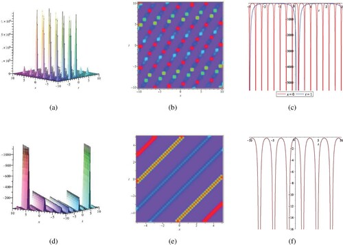Figure 4 showing the corresponding periodic blast solutions by $w_1$ taking c = 8 and ${\eta }_1$ taking c = 1. (b) and (e) are density plots, (c) and (f) are contour plots. Figure 5 illustrates the singular soliton solutions for $c=\frac{1}{2}$ in $w_2$ and c = 10 in ${\eta }_2$. It can be noticed by (c) and (f) that the shape of the wave does not change when x and t change. However, the amplitude of the wave is impacted when c is changed, and the amplitude increases as c. Figure 6 and Figure 7 depict the relevant structures of the corresponding periodic blasting solutions. From the figures it can be demonstrated that the solutions we derived are easily understood and the results are novel.

Figure 1. Kink wave solutions of w, η via (21(21) $\begin{array}{rl}& w\left(\tau \right)\\ & =-\frac{1}{24}{c}^2{\hslash }^2-\frac{1}{3}{c}^2\kappa +\frac{1}{4}{c}^2-1\\ & -\left(\frac{c^2\mathrm{\hslash \kappa }}{-\sqrt{{\hslash }^2-4\kappa }\tanh \left(\frac{\sqrt{{\hslash }^2-4\kappa }}{2}\left(\tau +c_1\right)\right)-\hslash }\right)\\ & -\frac{1}{2}\left(\frac{c^6{\hslash }^2{\kappa }^2}{{\left(-\sqrt{{\hslash }^2-4\kappa }\tanh \left(\frac{\sqrt{{\hslash }^2-4\kappa }}{2}\left(\tau +c_1\right)\right)-\hslash \right)}^2}\right),\end{array}$(21) ), (22(22) $\begin{array}{rl}& \eta \left(\tau \right)\\ & =-\frac{1}{12}c{\hslash }^2-\frac{2}{3}c\kappa +\frac{1}{2}c\\ & -\left(\frac{2c\mathrm{\hslash \kappa }}{-\sqrt{{\hslash }^2-4\kappa }\tanh \left(\frac{\sqrt{{\hslash }^2-4\kappa }}{2}\left(\tau +c_1\right)\right)-\hslash }\right)\\ & -\left(\frac{c^5{\hslash }^2{\kappa }^2}{{\left(-\sqrt{{\hslash }^2-4\kappa }\tanh \left(\frac{\sqrt{{\hslash }^2-4\kappa }}{2}\left(\tau +c_1\right)\right)-\hslash \right)}^2}\right).\end{array}$(22) ). (a) The 3D plot of w via (21); (b) Density plot of w; (c) Contour plot of w when x = 0, x = 1, t = 1, t = 5; (d) The 3D plot of η via (22); (e) Density plot of η; (f) Contour plot of η when x = 0, x = 1, t = 1, t = 5.

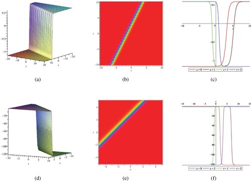
Figure 2. Traveling wave solutions of w, η via (23(23) $\begin{array}{rl}w\left(\tau \right)& =-\frac{1}{24}{c}^2{\hslash }^2-\frac{1}{3}{c}^2\kappa +\frac{1}{4}{c}^2-1\\ & -\frac{a_1\hslash }{2\left(\exp \left(\hslash \left(\tau +c_1\right)\right)-1\right)}\\ & -\frac{c^6{\hslash }^4}{8{\left(\exp \left(\hslash \left(\tau +c_1\right)\right)-1\right)}^2},\end{array}$(23) ), (24(24) $\begin{array}{rl}\eta \left(\tau \right)& =-\frac{1}{12}c{\hslash }^2-\frac{2}{3}c\kappa +\frac{1}{2}c\\ & -\frac{a_1\hslash }{c\left(\exp \left(\hslash \left(\tau +c_1\right)\right)-1\right)}\\ & -\frac{c^5{\hslash }^4}{4{\left(\exp \left(\hslash \left(\tau +c_1\right)\right)-1\right)}^2}.\end{array}$(24) ). (a) The 3D plot of w via (23); (b) Density plot of w; (c) Contour plot of w when x = 0, x = 1, t = 1, t = 10; (d) The 3D plot of η via (24); (e) Density plot of η; (f) Contour plot of η.

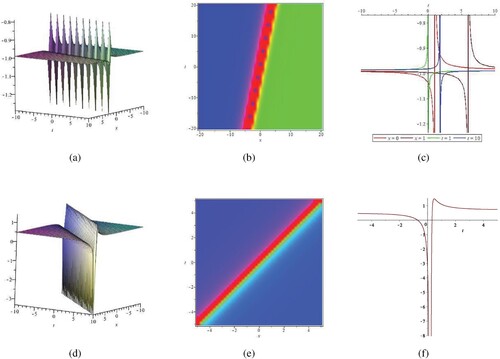
Figure 3. Periodic blast solutions of w, η via (29(29) $\begin{array}{rl}& w(\tau )\\ & =-\frac{1}{24}{c}^2{\hslash }^2-\frac{1}{3}{c}^2\kappa +\frac{1}{4}{c}^2-1\\ & -\frac{c^2\mathrm{\hslash \kappa }}{\sqrt{-{\hslash }^2+4\kappa }\tan \left(\frac{\sqrt{-{\hslash }^2+4\kappa }}{2}\left(\tau +c_1\right)\right)-\hslash }\\ & -\frac{c^2\mathrm{\hslash \kappa }}{2{\left(\sqrt{-{\hslash }^2+4\kappa }\tan \left(\frac{\sqrt{-{\hslash }^2+4\kappa }}{2}\left(\tau +c_1\right)\right)-\hslash \right)}^2},\end{array}$(29) ), (30(30) $\begin{array}{rl}& \eta (\tau )\\ & =-\frac{1}{12}c{\hslash }^2-\frac{2}{3}c\kappa +\frac{1}{2}c\\ & -\frac{c\mathrm{\hslash \kappa }}{2\sqrt{-{\hslash }^2+4\kappa }\tan \left(\frac{\sqrt{-{\hslash }^2+4\kappa }}{2}\left(\tau +c_1\right)\right)-2\hslash }\\ & -\frac{c\mathrm{\hslash \kappa }}{{\left(\sqrt{-{\hslash }^2+4\kappa }\tan \left(\frac{\sqrt{-{\hslash }^2+4\kappa }}{2}\left(\tau +c_1\right)\right)-\hslash \right)}^2}.\end{array}$(30) ). (a) The 3D plot of w via (29); (b) Density plot of w; (c) Contour plot of w when x = 0, t = 1; (d) The 3D plot of η via (30); (e) Density plot of η; (f) Contour plot of η when x = 0, t = 1.

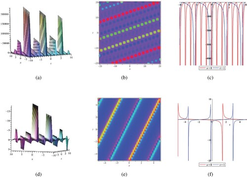
Figure 4. Travelling wave solutions of w, η via (35(35) $\begin{array}{rl}& \{\begin{array}{l}{w}_1=\frac{7c^2}{12}-1-\frac{c^2}{2}{\left(\tanh \tau \right)}^{-2},\\ {\eta }_1=\frac{7c}{6}-c{\left(\tanh \tau \right)}^{-2}.\end{array}\end{array}$(35) ). (a) The 3D plot of w via (35); (b) Density plot of w; (c) Contour plot of w when x = 0, x = 1, x = -1, t = 1, t = 2; (d) The 3D plot of η via (35); (e) Density plot of η; (f) Contour plot of η.

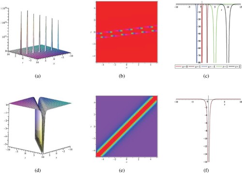
Figure 5. Singular soliton solutions of w, η via (36(36) $\begin{array}{rl}& \{\begin{array}{l}{w}_2=\frac{7c^2}{12}-1-\frac{c^2}{2}{\left(\coth \tau \right)}^{-2},\\ {\eta }_2=\frac{7c}{6}-c{\left(\coth \tau \right)}^{-2}.\end{array}\end{array}$(36) ). (a) The 3D plot of w via (36); (b) Density plot of w; (c) Contour plot of w when x = 0, x = 1, x = -1, t = 1, t = 2; (d) The 3D plot of η via (36); (e) Density plot of η; (f) Contour plot of η when c=1, c=5,c=10. (b), (c) are 2D and 3D plots related to w; (d), (e), (f) are 2D and 3D plots related to η.

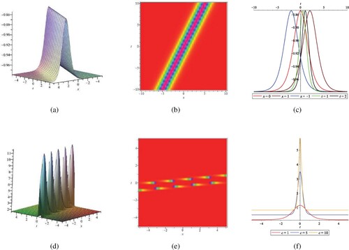
Figure 6. Periodic blasting solutions of w, η via (38(38) $\begin{array}{rl}& \{\begin{array}{l}{w}_4=-\frac{c^2}{12}-1-\frac{c^2}{2}{\left(\tanh \tau \right)}^{-2},\\ {\eta }_4=-\frac{c}{6}-c{\left(\tanh \tau \right)}^{-2}.\end{array}\end{array}$(38) ). (a) The 3D plot of w via (38); (b) Density plot of w; (c) Contour plot of w when x = 0, t = 1; (d) The 3D plot of η via (38); (e) Density plot of η; (f) Contour plot of η.

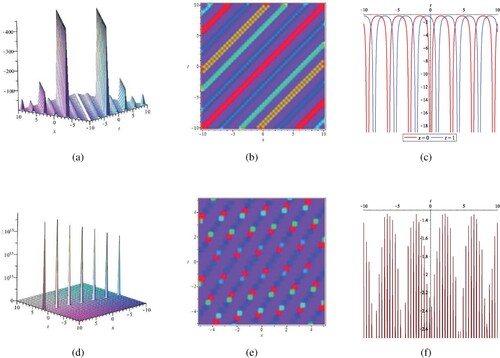
Figure 7. Periodic blasting solutions of w, η via (39(39) $\begin{array}{rl}& \{\begin{array}{l}{w}_5=-\frac{c^2}{12}-1-\frac{c^2}{2}{\left(\cot \tau \right)}^{-2},\\ {\eta }_5=-\frac{c}{6}-c{\left(\cot \tau \right)}^{-2}.\end{array}\end{array}$(39) ). (a) The 3D plot of w via (39); (b) Density plot of w; (c) Contour plot of w when x = 0, t = 1; (d) The 3D plot of η via (39); (e) Density plot of η; (f) Contour plot of η.

5. Conclusion

In this paper, the travelling wave solutions of the coupled BBM-KdV system were acquired using the exp$(-\varphi (\tau ))$ – expansion method, the modified extended tanh-function method and Kudryashov method. These solutions were expressed in terms of exponential functions, hyperbolic tangent functions and trigonometric functions. By using different expansions, solitary, periodic wave and kink solutions of the system (4(4) $\begin{array}{rl}& w_t+{\eta }_x+{\left(\mathrm{w\eta }\right)}_x-\frac{1}{6}{w}_{\mathrm{xxt}}=0,\\ & {\eta }_t+w_x+\eta {\eta }_x+\frac{1}{6}{w}_{\mathrm{xxx}}=0,\end{array}$(4) ) were obtained. The plots of the solutions by taking different values of the parameters, the dynamic behaviours of the solutions were observed more visually through these plots. Also, the geometries and behaviours of the solutions were analysed. On these basis, we compared the gained solutions with the existing solutions, and the results of this paper enriched the kinds of solutions of the BBM-KdV model. BBM-KdV has been broadly applied as a shallow water wave model for the simulation of waves in coastal and offshore engineering. Consequently, the results of this paper can be useful for the research of wave motion patterns and can provide reasonable bases for the implementation of offshore projects.

Disclosure statement

No potential conflict of interest was reported by the author(s).

Additional information

Funding

The work was supported in part by Young Scientists Fund (CN)(Grant No. 11001115, No. 11201473), Natural Science Foundation of Shandong Province (Grant ZR2021MA084) and the Natural Science Foundation of Liaocheng University (318012025).

References

- Boussinesq J. Thorie des ondes et des remous qui se propagent le long d'un canal rectangulaire horizontal, en communiquant au liquide contenu dans ce canal des vitesses sensiblement pareilles de la surface au fond. J Math Pures Appl. 1872;17:55–108.
- Benjamin TB, Bona JL, Mahony JJ. Model equations for long waves in nonlinear dispersive systems. Philos Trans R Soc B Biol Sci. 1972;272(1220):47–78.
- Raslan KR, Ali KK, Danaf TS. Numerical treatment for the coupled-BBM system. J Modern Methods Numer Math. 2016;7(2):67–79. doi: 10.20454/jmmnm.2016.1093
- Kumar V. Modified (G′/G)-expansion method for finding traveling wave solutions of the coupled Benjamin-Bona-Mahony-kdv equation. J Ocean Eng Sci. 2019;4(3):252–255. doi: 10.1016/j.joes.2019.04.008
- Raslan KR, Ali KK, Danaf TS. An efficient approach to numerical study of the coupled-bbm system with b-spline collocation method. Commun Math Model Appl. 2016;1(3):5–15.
- Wu WJ, Manafian J, Ali KK, et al. Numerical and analytical results of the 1D BBM equation and 2D coupled BBM-system by finite element method. Int J Modern Phys. 2022;36(28):2250201. doi: 10.1142/S0217979222502010
- Antonopoulos DC, Dougalis VA, Mitsotakis DE. Numerical solution of Boussinesq systems of the Bona-Smith family. Appl Numer Math. 2010;60(4):314–336. doi: 10.1016/j.apnum.2009.03.002
- Dougalis VA, Mitsotakis DE, Saut JC. Boussinesq system of Bona-Smith type on plane domains: theory and numerical analysis. J Sci Comput. 2010;44:109–135. doi: 10.1007/s10915-010-9368-z
- Karakoc SBG, Bhowmik SK. Galerkin finite element solution for Benjamin-Bona-Mahony-Burgers equation with cubic B-Splines. Comput Math Appl. 2019;77(7):1917–1932.
- Yagmurlu NM, Uçar Y, Çelikkaya İ. Higher order splitting method for numerical solution of nonlinear coupled system viscous burger's equation. Konuralp J Math. 2020;8(2):234–243.
- Tasbozan O. Approximate analytical solutions of fractional coupled mKdV equation by homotopy analysis method. Open J Appl Sci. 2012;02(03):193–197. doi: 10.4236/ojapps.2012.23029
- Aziz N, Ali K, Seadawy AR, et al. Discussion on couple of nonlinear models for lie symmetry analysis, self adjointees, conservation laws and soliton solutions. Opt Quantum Electron. 2023;55(3):201. doi: 10.1007/s11082-022-04416-x
- Yin JL, Tian LX. Classification of the travelling waves in the nonlinear dispersive kdV equation. Nonlinear Anal. 2010;73(2):465–470. doi: 10.1016/j.na.2010.03.039
- Nguetcho AST, Li JB, Bilbault JM. Global dynamical behaviors in a physical shallow water system. Commun Nonlinear Sci Numer Simul. 2016;36:285–302. doi: 10.1016/j.cnsns.2015.12.006
- Li JB, Zhang Y. Solitary wave and chaotic behavior of traveling wave solutions for the coupled kdV equations. Appl Math Comput. 2011;218(5):1794–1797.
- Seadawy AR, Rizvi STR, Ahmed S. Analytical solutions along with grey-black optical solitons under the influence of self-steepening effect and third order dispersion. Opt Quantum Electron. 2023;55(3):288. doi: 10.1007/s11082-023-04559-5
- Seadawy AR, Rizvi STR, Ahmed S, et al. Propagation of W-shaped and M-shaped solitons with multi-peak interaction for ultrashort light pulse in fibers. Opt Quantum Electron. 2023;55(3):221. doi: 10.1007/s11082-022-04478-x
- Seadawy AR, Rizvi STR, Ahmad A. Study of non-local Boussinesq dynamical equation for multiwave, homoclinic breathers and other rational solutions. Opt Quantum Electron. 2023;55(3):278. doi: 10.1007/s11082-023-04550-0
- Seadawy AR, Rizvi STR, Shabbir S, et al. Study of localized waves for couple of the nonlinear Schrödinger dynamical equations. Int J Modern Phys B. 2023;37(05):2350047. doi: 10.1142/S0217979223500479
- Zhang YS, Rao JG, Cheng Y, et al. Riemann-Hilbert method for the Wadati-Konno-Ichikawa equation: N simple poles and one higher-order pole. Phys D: Nonlinear Phenom. 2019;399(1):173–185. doi: 10.1016/j.physd.2019.05.008
- Gurefe Y, Sonmezoglu A, Misirli E. Application of the trial equation method for solving some nonlinear evolution equations arising in mathematical physics. Pramana. 2011;77(6):1023–1029. doi: 10.1007/s12043-011-0201-5
- Du XH. An irrational trial equation method and its applications. Pramana, J Phys. 2010;75(3):415–422. doi: 10.1007/s12043-010-0127-3
- Gepreel KA. Extended trial equation method for nonlinear coupled Schrodinger Boussinesq partial differential equations. J Egypt Math Soc. 2016;24(3):381–391. doi: 10.1016/j.joems.2015.08.007
- Rizvi STR, Seadawy AR, Ahmed S, et al. Einstein's vacuum field equation: lumps, manifold periodic, generalized breathers, interactions and rogue wave solutions. Opt Quantum Electron. 2023;55(2):181. doi: 10.1007/s11082-022-04451-8
- Seadawy AR, Rizvi STR, Ahmed S, et al. Lump solutions, Kuznetsov-Ma breathers, rogue waves and interaction solutions for magneto electro-elastic circular rod. Chaos Solitons Fract. 2022;163:112563. doi: 10.1016/j.chaos.2022.112563
- Wang KJ, Liu JH, Si J, et al. N-Soliton, breather, lump solutions and diverse traveling wave solutions of the fractional (2+1)-dimensional Boussinesq equation. Fractals. 2023;31(03):2350023. doi: 10.1142/S0218348X23500238
- Younas U, Seadawy AR, Younis M, et al. Construction of analytical wave solutions to the conformable fractional dynamical system of ion sound and Langmuir waves. Waves Random Complex Media. 2022;32(6):2587–2605. doi: 10.1080/17455030.2020.1857463
- Wang KJ, Liu JH. Diverse optical solitons to the nonlinear Schrödinger equation via two novel techniques. Eur Phys J Plus. 2023;138(1):74. doi: 10.1140/epjp/s13360-023-03710-1
- Wang KJ. A fast insight into the optical solitons of the generalized third-order nonlinear Schrödinger's equation. Res Phys. 2022;40:105872.
- Khan K, Akbar MA. Traveling wave solutions of nonlinear evolution equations via the enhanced (G′/G)-expansion method. J Egypt Math Soc. 2014;22(2):220–226. doi: 10.1016/j.joems.2013.07.009
- Zhang S. Application of exp-function method to high-dimensional nonlinear evolution equation. Chaos, Solitons & Fractals. 2008;38(1):270–276. doi: 10.1016/j.chaos.2006.11.014
- Rizvi STR, Seadawy AR, Younis M, et al. Optical dromions for complex Ginzburg Landau model with nonlinear media. Appl Math A J Chin Universities. 2023;38(1):111–125. doi: 10.1007/s11766-023-4044-x
- Rizvi STR, Seadawy AR, Ahmed S, et al. Optical soliton solutions and various breathers lump interaction solutions with periodic wave for nonlinear Schrödinger equation with quadratic nonlinear susceptibility. Opt Quantum Electron. 2023;55(3):286. doi: 10.1007/s11082-022-04402-3
- Rizvi STR, Seadawy AR, Naqvi SK, et al. Study of mixed derivative nonlinear Schrödinger equation for rogue and lump waves, breathers and their interaction solutions with Kerr law. Opt Quantum Electron. 2023;55(2):177. doi: 10.1007/s11082-022-04415-y
- Batool T, Seadawy AR, Rizvi STR, et al. Optical multi-wave, M-shaped rational solution, homoclinic breather, periodic cross-kink and various rational solutions with interactions for radhakrishnan-Kundu-Lakshmanan dynamical model. J Nonlinear Opt Phys Mater. 2023;32(02):2350015. doi: 10.1142/S0218863523500157
- Rizvi STR, Seadawy AR, Raza U. Some advanced chirped pulses for generalized mixed nonlinear Schrödinger dynamical equation. Chaos, Solitons & Fractals. 2022;163:112575. doi: 10.1016/j.chaos.2022.112575
- Wang KJ, Si J. Diverse optical solitons to the complex Ginzburg-Landau equation with Kerr law nonlinearity in the nonlinear optical fiber. Eur Phys J Plus. 2023;138(3):187. doi: 10.1140/epjp/s13360-023-03804-w
- Wang KJ, Shi F, Wang GD. Abundant soliton structures to the (2+1)-Dimensional heisenberg ferromagnetic spin chain dynamical model. Adv Math Phys. 2023;2023:4348758.
- Wang KJ. Diverse wave structures to the modified Benjamin-Bona-Mahony equation in the optical illusions field. Modern Phys Lett B. 2023;37:2350012. doi: 10.1142/S0217984923500124
- Inan IE, Inc M, Martinez HY, et al. Extended exp(−φ(ξ))-expansion method for some exact solutions of (2+1) and (3+1)-dimensional constant coefficients kdV equations. J Ocean Eng Sci. 2022.
- Arshed S. New soliton solutions to the perturbed nonlinear Schrödinger equation by exp(−ϕ(ξ))-expansion method. Optik. 2020;220:165123. doi: 10.1016/j.ijleo.2020.165123
- Akbulut A, Kaplan M, Tascan F. The investigation of exact solutions of nonlinear partial differential equations by using exp(−ϕ(ξ)) method. Optik. 2017;132:382–387. doi: 10.1016/j.ijleo.2016.12.050
- Ahmed MS, Zaghrout AAS, Ahmed HM. Travelling wave solutions for the doubly dispersive equation using improved modified extended tanh-function method. 2022;61(10):7987–7994.
- Karakoc SBG, Ali KK. Theoretical and computational structures on solitary wave solutions of Benjamin Bona Mahony-Burgers equation. Tbil Math J. 2021;14(2):33–50.
- Bashar H, Rista TT, Shahen NHM. Application of the advanced exp (−ϕ(ξ))-Expansion method to the nonlinear conformable time-Fractional partial differential equations. Turk J Math Comput Sci. 2021;13(1):68–80.
- Alam LMB, Jiang XF, Mamun AA. Exact and explicit traveling wave solution to the time-fractional phi-four and (2+1) dimensional CBS equations using the modified extended tanh-function method in mathematical physics. Partial Differ Equ Appl Math. 2021;4:100039. doi: 10.1016/j.padiff.2021.100039
- Hubert MB, Betchewe G, Doka SY, et al. Soliton wave solutions for the nonlinear transmission line using the Kudryashov method and the (G′/G)-expansion method. Appl Math Comput. 2014;239:299–309.