Preliminary evaluation of MJO simulation in GAMIL3 (Grid-point atmospheric model of IAP LASG)

ABSTRACT

This study evaluates the performance of the Grid-point Atmospheric Model of IAP LASG, version 3 (GAMIL3), in simulating the Madden–Julian Oscillation (MJO), based on the CMIP6 (phase 6 of the Coupled Model Intercomparison Project) AMIP (Atmospheric Model Intercomparison Project) simulation. Results show that GAMIL3 reasonably captures the main features of the MJO, such as the eastward-propagating signal in the MJO frequency band, the symmetric and asymmetric structures of the MJO, several convectively coupled equatorial waves, and the MJO life cycle. However, GAMIL3 underestimates the MJO amplitude, especially for outgoing longwave radiation, as do most CMIP5 models, and simulates slow eastward propagation.

GRAPHICAL ABSTRACT

摘要

本文以第六次国际耦合模式比较计划（CMIP6）的 大气模式比较（AMIP）试验结果为基础，评估了中国科学院大气物理研究所LASG国家重点实验室所研发的新版本格点大气环流模式GAMIL3对MJO的模拟性能。结果表明：GAMIL3合理地捕捉了MJO的主要特征，如MJO向东传播的信号、MJO的对称和非对称结构、几种对流耦合的赤道波动以及MJO的生命周期。然而，正如大多数CMIP5模型一样GAMIL3低估了MJO的振幅，和东传速度。

KEYWORDS:

• MJO
• GAMIL3
• evaluation

关键词:

• 热带季节内振荡
• 格点大气环流模式
• 模式评估

1. Introduction

In the early 1970s, Madden and Julian (1971, 1972) found a quasi-periodic oscillation in the atmosphere near the equator on a time scale of 40–50 days. Subsequent studies have shown 30–60-day quasi-periodic oscillations throughout the tropical atmosphere, and even the global atmosphere, and this is regarded as one of the most important atmospheric circulation systems (Krishinamurti and Subrahmann 1982; Li 1983; Knuston and Weickmann 1987; Liebmann, Hendon, and Glick 1994). Such intraseasonal atmospheric oscillations near the equator are referred to as the Madden–Julian Oscillation (MJO).

Observations and numerical simulations have indicated that the MJO has great influence on tropical weather and climate phenomena, including the Indian Ocean summer monsoon, the Australian winter monsoon, the South China Sea summer monsoon, tropical cyclone activity, and El–Niño Southern Oscillation (Yasunari 1979, 1980; Hall, Matthews, and Karoly 2001; Li and Long 2001; Annamalai and Sperber 2005; Lorenz and Hartmann 2006; Wheeler et al. 2009; Wang et al. 2017a). The MJO also influences the weather and climate outside the tropics through atmospheric teleconnection mechanisms (Weickmann, Lussky, and Kutzbach 1985; Ferranti et al. 1990; Lin, Brunet, and Derome 2009; Henderson, Maloney, and Barnes 2016) and modulates the global climate (Wang et al. 2013; Wang, Li, and Chen 2019; Chen, Yu, and Zheng 2016; Chen et al. 2017).

However, current atmospheric models have difficulty in providing realistic MJO simulations (Slingo et al. 1996). An evaluation of MJO simulation performance of models participating in phase 5 of the Coupled Model Intercomparison Project (CMIP5; Hung et al. 2013; Ahn et al. 2017) found that most models underestimate the MJO amplitude, and that the simulated MJO propagation is fast compared with observations. Moreover, the symmetry and asymmetry of the convectively coupled Kelvin waves (CCKWs) between the Northern and Southern Hemisphere using the CMIP5 coupled models were evaluated, suggesting that some models overestimate the amplitude of CCKWs in the Southern Hemisphere (Wang and Li, 2017). In operational MJO prediction, assimilating the observed surface signals is considered as the minimum requirement (Cui et al. 2020).

The Grid-point Atmospheric Model of IAP LASG (GAMIL) was developed at the State Key Laboratory of Numerical Modeling for Atmospheric Sciences and Geophysical Fluid Dynamics (LASG), Institute of Atmospheric Physics (IAP), Chinese Academy of Sciences, Beijing, China. The simulation performance for the MJO and other intraseasonal oscillations by early versions of the model (GAMIL1 and GAMIL2) has been evaluated previously (Yang et al. 2009; Mao and Li 2012; Xie et al. 2012). The newest version (GAMIL3) has recently been developed and has completed the Atmospheric Model Intercomparison Project (AMIP) runs of phase 6 of the Coupled Model Intercomparison Project (CMIP6). This paper evaluates the ability of GAMIL3 to simulate the MJO. Descriptions of the model and observational data are presented in section 2. Section 3 evaluates the performance of MJO simulations. Finally, a summary and discussion are presented in section 4.

2. Model and observational data

GAMIL3 uses a hybrid 2D decomposition to improve parallel scalability (Liu et al. 2014). The horizontal resolution is ~2°, with a 180 × 80 longitude–latitude grid, and the vertical resolution is 26 layers from the surface to the top of the model (2.194 hPa) with an σ-coordinate system. To improve water vapor conservation, the weight of the two-step shape-preserving advection scheme of the previous version (GAMIL2; Li et al. 2013) has been modified in GAMIL3. A planetary boundary layer scheme based on turbulence kinetic energy and a stratocumulus cloud-fraction scheme based on estimated inversion strength are adopted in GAMIL3 (Guo and Zhou 2014; Sun, Li, and Wang 2016). In addition, the convective momentum transport and the simple parameterization to describe anthropogenic aerosol effects recommended by CMIP6 have been added (Stevens et al. 2017; Shi, Zhang, and Liu 2019). Following CMIP6 recommendations, the external forcings, such as greenhouse gases, ozone, land use, the solar constant, and aerosols, have also been updated (https://esgf-node.llnl.gov/search/input4mips/).

In this paper, AMIP runs for the years 1980–2005 are analyzed following the CLIVAR (U.S. Climate Variability and Predictability) MJO Working Group’s diagnostics package. We mainly use daily data and apply a 20–100-day Lanczos bandpass filter (Waliser et al. 2009). The analysis will focus on boreal winter.

To verify the model results, the following observation/reanalysis datasets are used: satellite-observed daily outgoing longwave radiation (OLR) from the Advanced Very High Resolution Radiometer (AVHRR; Liebmann and Smith 1996); and upper-tropospheric (200 hPa) and lower-tropospheric (850 hPa) winds from NCEP–NCAR reanalysis data (Kalnay et al. 1996).

3. Preliminary evaluation of MJO simulation in GAMIL3

The 20–100-day-filtered 850-hPa zonal wind (U850) during boreal winter (November–April) and its percentage contribution to the overall variance are shown in Figure 1. Large percentage values are seen over the tropical Indian Ocean (35%–40%), the Maritime Continent (> 40%), and the tropical and northern Pacific Ocean (35%–40%) in the NCEP–NCAR reanalysis (Figure 1(a)). GAMIL3 captures the above spatial distribution of large percentage values well, especially over the central Maritime Continent (Figure 1(c)). The spatial distribution of OLR variance (Figure 1(b,d)) is similar to that of U850. Two east–west band-shaped large-variance-percentage belts are located over the northern and southern Indian Ocean in GAMIL3, whereas one region of large variance is located over the tropical Indian Ocean in observations (Figure 1(b,d)). GAMIL3 also has a negative variance percentage bias over the Maritime Continent.

Figure 1. 20–100-day band-pass-filtered U850 variance (contours; units: m² s⁻²) and its percentage contribution (shaded) to the total variance in (a) NCEP–NCAR reanalysis and (c) GAMIL3. (b, d) As in (a, c) but for OLR (units: W² m⁻⁴) from NOAA AVHRR and GAMIL3, respectively

Figure 2 shows the wavenumber-frequency power spectra of 10°S–10°N-averaged OLR and U850, which provides a convenient metric of MJO characteristics. The observed spectral power of U850 and OLR are concentrated over the domain of eastward wavenumbers 1–3, with periods of 30–80 days (Figure 2(a,c)). The model contains significant eastward-propagating signals in the MJO band for both OLR and U850. However, the simulated energy is smaller than observations of OLR and the dominant peak is outside of the MJO band in U850 (Figure 2(b,d), similar to other atmospheric general circulation model simulations (e.g., ECHAM6; Crueger, Stevens, and Brokopf 2013). The eastward/westward (E/W) ratio, which is obtained by dividing the sum of spectral power over the MJO band by that of its westward propagating counterpart, and the eastward/observation (E/O) ratio, which is formulated by normalizing the sum of spectral power within the MJO band by the observed value, are calculated from frequency–wavenumber spectra, and are metrics used to indicate the robustness of eastward-propagating features of the MJO (Table 1). The observed (simulated) E/W ratios are 3.7 (1.7) and 3.8 (2.9) for OLR and U850, respectively. The E/O ratio is 0.4 for OLR and 0.9 for U850 in GAMIL3. These results indicate that the model generally underestimates the eastward propagation of convection, but the simulation of the eastward propagation of circulation is much better. These results are similar to those from most CMIP5 coupled models (Subramanian et al. 2011; Ahn et al. 2017).

Table 1. Eastward/westward (E/W) and eastward/observation (E/O) ratios within the MJO frequency–wavenumber ranges (30–80-day period, wavenumbers 1–3) for the single equatorial fields of OLR and U850

	E/W Ratio		E/O Ratio
	OLR	U850	OLR	U850
Observations	3.7	3.8	1	1
GAMIL3	1.7	2.9	0.4	0.9

Figure 2. November–April (1980–2005) wavenumber–frequency spectra of 10°N–10°S-averaged daily U850 from (a) NCEP and (b) GAMIL3; and daily OLR fields from (c) NOAA satellite OLR and (d) GAMIL3. The dashed lines indicate the MJO band (30 d to 80 d)

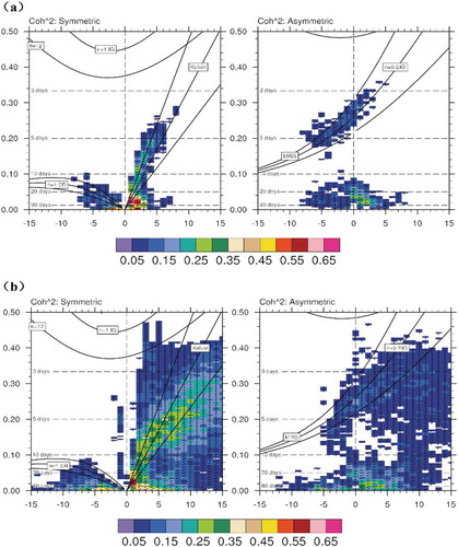
We can clearly distinguish the main MJO modes and convectively coupled equatorial waves (CCEWs), including Kelvin, equatorial Rossby, mixed Rossby–gravity, and eastward inertia-gravity waves, through the coherence-squared and phase relationship between equatorial OLR and U850 for the symmetric and asymmetric components (Figure 3). In the MJO band, observations show high coherence and an approximate 90° phase lag between convection and 850-hPa winds (Figure 3(a)). The GAMIL3 simulation is almost consistent with observational data and effectively reproduces the MJO and several CCEWs—both the symmetric and asymmetric components (Figure 3(b). For wavenumber 1, model coherence peaks are close to observations in both the symmetric and asymmetric structures and demonstrate the existence of the MJO in the model. For wavenumbers 2 and 3, GAMIL3 has significant coherence with observations in asymmetric structure, but lower coherence in symmetric structure.

Figure 3. Coherence-squared (colors) and phase relationships (vectors) between U850 and OLR for (a) NCEP winds and satellite OLR, and (b) GAMIL3 winds and OLR simulation. Colors represent coherence-squared between OLR and U850, and vectors represent the phase by which wind anomalies lag OLR anomalies, increasing in the clockwise direction

Eight phases of the MJO life cycle from observations and the model run are shown in Figure 4, following the method of Waliser et al. (2009). MJO convection forms over the Indian Ocean and spreads southeastward. It then passes through the Maritime Continent and finally reaches a region near the International Date Line (IDL; Figure 4(a). GAMIL3 is able to capture the overall eastward propagation of convection. That is, convection is generated near the equator in the Indian Ocean, then propagates eastward, and finally terminates around the Maritime Continent (Figure 4(b). However, the convection is weak, consistent with underestimates of the eastward propagation of convection in Figure 2(d. Moreover, the convective propagation speed of the model is slow and fails to reach the IDL. In general, GAMIL3 has some ability to simulate the MJO. However, the simulated signal is weak and the propagation is slow.

Figure 4. Composite MJO OLR (shaded; units W m⁻²) and 850-hPa wind anomalies (vectors; units: m s⁻¹) in eight phases from November to April from (a) observations and (b) GAMIL3. The reference vector in units of m s⁻¹ is in the upper right, and the phase and number of days used are in the lower right, of each panel

4. Summary and discussion

This study evaluates MJO simulations of GAMIL3 using CMIP6 AMIP-type runs. Results show that GAMIL3 can simulate the main features of the MJO. For example, the model generally simulates the variance of U850 and OLR over the tropics. However, the eastward-propagating signal in both OLR and U850 from the power during the MJO band is weaker than in observations. In general, the simulated circulation is better than that of OLR. GAMIL3 is also able to effectively reproduce both symmetric and asymmetric waves. The MJO and several CCEWs are closely consistent with observational data, exhibiting strong coherence in the MJO band. Phase lags between equatorial OLR and U850 are similar to those of observations. The model also simulates the MJO life cycle well. However, it underestimates the MJO amplitude, especially as it relates to OLR, as do most CMIP5 models (Hung et al. 2013; Jiang et al. 2015). This is related to poor climatological mean simulations of Indian Ocean OLR and precipitation in GAMIL3.

Although GAMIL3 can simulate the basic characteristics of the MJO, there is still room for improvement. For example, convective parameterization is considered as the critical process for MJO simulation (Crueger, Stevens, and Brokopf 2013; Wang et al. 2017b). However, before concentrating on this aspect, it is necessary to evaluate the contributions of each model improvement (including convective parameterization) in GAMIL3 to MJO simulations relative to the previous model version, applying the new dynamics-oriented diagnostics for the MJO proposed by Wang et al. (2018). In addition, many previous studies have shown air–sea interactions play an important role in the MJO (Crueger, Stevens, and Brokopf 2013; Jiang et al. 2015). Further analysis is needed using results of the coupled FGOALS-g3 model.

Disclosure statement

No potential conflict of interest was reported by the authors.

Additional information

Funding

This study was jointly supported by the National Key Research and Development Program of China [grant number 2017YFA0603903] and the National Natural Science Foundation of China [grant numbers 41622503 and 41775101].

References

- Ahn, M. S., D. Kim, K. R. Sperber, I. S. Kang, E. Maloney, D. Waliser, H. Hendon, et al. 2017. “MJO Simulation in CMIP5 Climate Models: MJO Skill Metrics and Process-oriented Diagnosis.” Climate Dynamics 49 (5): 1–23. doi:10.1007/s00382-017-3558-4.
- Annamalai, H., and K. R. Sperber. 2005. “Regional Heat Sources and the Active and Break Phases of Boreal Summer Intraseasonal (30–50 Day) Variability.” Journal of the Atmospheric Sciences 62 (8): 2726–2748. doi:10.1175/JAS3504.1.
- Chen, L., T. Li, B. Wang, and L. Wang. 2017. “Formation Mechanism for 2015/16 Super El Niño.” Scientific Reports 7 (1): 2975. doi:10.1038/s41598-017-02926-3.
- Chen, L., Y. Yu, and W. Zheng. 2016. “Improved ENSO Simulation from Climate System Model FGOALS-g1.0 To FGOALS-g2.” Climate Dynamics 47 (7–8): 2617–2634. doi:10.1007/s00382-016-2988-8.
- Crueger, T., B. Stevens, and R. Brokopf. 2013. “The Madden–Julian Oscillation in ECHAM6 and the Introduction of an Objective MJO Metric.” Journal of Climate 26 (10): 3241–3257. doi:10.1175/JCLI-D-12-00413.1.
- Cui, J. X., L. Wang, T. Li, and B. Wu. 2020. “Can Reanalysis Products with Only Surface Variables Assimilated Capture Madden–Julian Oscillation Characteristics?” International Journal of Climatology 40 (2): 1279–1293. doi:10.1002/joc.6270.
- Ferranti, L., T. N. Palmer, F. Molteni, and E. Klinker. 1990. “Tropical-extratropical Interaction Associated with the 30–60 Day Oscillation and Its Impact on Medium and Extended Range Prediction.” Journal of the Atmospheric Sciences 47 (18): 2177–2199. doi:10.1175/1520-0469(1990)047<2177:TEIAWT>2.0.CO;2.
- Guo, Z., and T. J. Zhou. 2014. “An Improved Diagnostic Stratocumulus Scheme Based on Estimated Inversion Strength and Its Performance in GAMIL2.” Science China Earth Sciences 57 (11): 2637–2649. doi:10.1007/s11430-014-4891-7.
- Hall, J. D., A. J. Matthews, and D. J. Karoly. 2001. “The Modulation of Tropical Cyclone Activity in Australian Region by the Madden-Julian Oscillation.” Monthly Weather Review 129 (12): 2970–2982. doi:10.1175/1520-0493(2001)129<2970:TMOTCA>2.0.CO;2.
- Henderson, S. A., E. D. Maloney, and E. A. Barnes. 2016. “The Influence of the Madden-Julian Oscillation on Northern Hemisphere Winter Blocking.” Journal of Climate 29 (12): 4597–4616. doi:10.1175/JCLI-D-15-0502.1.
- Hung, M. P., J. L. Lin, W. Wang, D. Kim, T. Shinoda, and S. Weaver. 2013. “MJO and Convectively Coupled Equatorial Waves Simulated by CMIP5 Climate Models.” Journal of Climate 26 (17): 6185–6214. doi:10.1175/JCLI-D-12-00541.1.
- Jiang, X., D. E. Waliser, P. K. Xavier, J. Petch, N. P. Klingaman, S. J. Woolnough, B. Guan, et al. 2015. “Vertical Structure and Physical Processes of the Madden-Julian Oscillation: Exploring Key Model Physics in Climate Simulations.” Journal of Geophysical Research: Atmospheres 120 (10): 4718–4748. doi:10.1002/2014JD022375.
- Kalnay, E., M. Kanamitsu, R. Kistler, W. Collins, D. Deaven, L. Gandin, M. Iredell, et al. 1996. “The NCEP/NCAR 40-Year Reanalysis Project.” Bulletin of the American Meteorological Society 77 (3): 437–471. doi:10.1175/1520-0477(1996)077<0437:TNYRP>2.0.CO;2.
- Knuston, T. R., and K. M. Weickmann. 1987. “30–60 Day Atmospheric Oscillation: Composite Life Cycles of Convection and Circulation Anomalies.” Monthly Weather Review 115 (7): 1407–1436. doi:10.1175/1520-0493(1987)115<1407:DAOCLC>2.0.CO;2.
- Krishinamurti, T. N., and D. Subrahmann. 1982. “The 30–50 Day Mode at 850 Mb during MONEX.” Journal of the Atmospheric Sciences 39 (9): 2088–2095. doi:10.1175/1520-0469(1982)039<2088:TDMAMD>2.0.CO;2.
- Li, C. Y. 1983. “Convective Condensation Heating and Unstable Mode.” Chinese Journal of Atmospheric Sciences (In Chinese) 7 (3): 260–268. doi:10.3878/j.issn.1006-9895.1983.03.03.
- Li, C. Y., and Z. X. Long. 2001. “Intraseasonal Oscillation Anomalies in the Tropical Atmosphere and the 1997 El Niño Occurrence.” Chinese Journal of Atmospheric Sciences (In Chinese) 25: 337–345. doi:10.3878/j.issn.1006-9895.2001.05.02.
- Li, L., B. Wang, L. Dong, L. Liu, S. Shen, N. Hu, W. Sun, et al. 2013. “Evaluation of Grid-point Atmospheric Model of IAP LASG Version 2.0 (GAMIL2).” Advances in Atmospheric Sciences 30 (3): 855–867. doi:10.1007/s00376-013-2157-5.
- Liebmann, B., and C. Smith. 1996. “Description of a Complete (Interpolated) Outgoing Longwave Radiation Dataset.” Bulletin of the American Meteorological Society 77: 1275–1277. doi:10.1175/1520-0477(1996)077<1255:EA>2.0.CO;2.
- Liebmann, B., H. H. Hendon, and J. D. Glick. 1994. “The Relationship between Tropical Cyclones of the Western Pacific and Indian Oceans and the Madden-Julian Oscillation.” Journal of the Meteorological Society of Japan. Ser. II 72 (3): 401–412. doi:10.2151/jmsj1965.72.3_401.
- Lin, H., G. Brunet, and J. Derome. 2009. “An Observed Connection between the North Atlantic Oscillation and the Madden–Julian Oscillation.” Journal of Climate 22 (2): 364–380. doi:10.1175/2008jcli2515.1.
- Liu, L., R. Li, G. Yang, B. Wang, L. Li, and Y. Pu. 2014. “Improving Parallel Performance of a Finite-Difference AGCM on Modern High-Performance Computers.” Journal of Atmospheric and Oceanic Technology 31 (10): 2157–2168. doi:10.1175/jtech-d-13-00067.1.
- Lorenz, D. J., and D. L. Hartmann. 2006. “The Effect of the MJO on the North American Monsoon.” Journal of Climate 19 (3): 333–343. doi:10.1175/jcli3684.1.
- Madden, R., and P. Julian. 1971. “Detection of a 40–50 Day Oscillation in the Zonal Wind in the Tropical Pacific.” Journal of the Atmospheric Sciences 28 (5): 702–708. doi:10.1175/1520-0469(1971)028<0702:DOADOI>2.0.CO;2.
- Madden, R., and P. Julian. 1972. “Description of Global-scale Circulation Cells in the Tropics with a 40–50 Day Period.” Journal of the Atmospheric Sciences 29 (6): 1109–1123. doi:10.1175/1520-0469(1972)029<1109:dogscc>2.0.co;2.
- Mao, J. Y., and L. J. Li. 2012. “An Assessment of MJO and Tropical Waves Simulated by Different Versions of the GAMIL Model.” Atmospheric and Oceanic Science Letters 5,26–31. doi:10.1080/16742834.2012.11446960.
- Shi, X. J., W. T. Zhang, and J. J. Liu. 2019. “Comparison of Anthropogenic Aerosol Climate Effects among Three Climate Models with Reduced Complexity.” Atmosphere 10 (8): 456. doi:10.3390/atmos10080456.
- Slingo, J. M., K. R. Sperber, J. S. Boyle, J. P. Ceron, M. Dix, B. Dugas, W. Ebisuzaki, et al. 1996. “Intraseasonal Oscillations in 15 Atmospheric General Circulation Models: Results from an AMIP Diagnostic Subproject.” Climate Dynamics 12 (5): 325–357. doi:10.1007/BF00231106.
- Stevens, B., S. Fiedler, S. Kinne, K. Peters, S. Rast, J. Muesse, S. J. Smith, and T. Mauritsen. 2017. “MACv2-SP: A Parameterization of Anthropogenic Aerosol Optical Properties and an Associated Twomey Effect for Use in CMIP6.” Geoscientific Model Development 10 (1): 433–452. doi:10.5194/gmd-10-433-2017.
- Subramanian, A. C., M. Jochum, A. J. Miller, R. Murtugudde, R. B. Neale, and D. E. Waliser. 2011. “The Madden–Julian Oscillation in CCSM4.” Journal of Climate 24 (24): 6261–6282. doi:10.1175/jcli-d-11-00031.1.
- Sun, W. Q., L. J. Li, and B. Wang. 2016. “Reducing the Biases in Shortwave Cloud Radiative Forcing in Tropical and Subtropical Regions from the Perspective of Boundary Layer Processes.” Science China Earth Sciences 59 (7): 1427–1439. doi:10.1007/s11430-016-5290-z.
- Waliser, D., K. Sperber, H. Hendon, D. Kim, E. D. Maloney, M. C. Wheeler, K. M. Weickmann, et al. 2009. “MJO Simulation Diagnostics.” Journal of Climate 22 (11): 3006–3030. doi:10.1175/2008JCLI2731.1.
- Wang, B., S. Lee, D. E. Waliser, C. Zhang, A. Sobel, E. Maloney, T. Li, X. Jiang, and K. J. Ha. 2018. “Dynamics-Oriented Diagnostics for the Madden–Julian Oscillation.” Journal of Climate 31 (8): 3117–3135. doi:10.1175/JCLI-D-17-0332.1.
- Wang, H., F. Liu, B. Wang, and T. Li. 2017a. “Effects of Intraseasonal Oscillation on South China Sea Summer Monsoon Onset.” Climate Dynamics 1–16. doi:10.1007/s00382-017-4027-9.
- Wang, L., and T. Li. 2017. “Convectively Coupled Kelvin Waves in CMIP5 Coupled Climate Models.” Climate Dynamics 48 (3): 767–781. doi:10.1007/s00382-016-3109-4.
- Wang, L., T. Li, E. Maloney, and B. Wang. 2017b. “Fundamental Causes of Propagating and Nonpropagating MJOs in MJOTF/GASS Models.” Journal of Climate 30 (10): 3743–3769. doi:10.1175/JCLI-D-16-0765.1.
- Wang, L., T. Li, and L. Chen. 2019. “Modulation of the Madden–Julian Oscillation on the Energetics of Wintertime Synoptic-scale Disturbances.” Climate Dynamics 52 (7–8): 4861–4871. doi:10.1007/s00382-018-4447-1.
- Wang, L., T. Li, T. Zhou, and X. Rong. 2013. “Origin of the Intraseasonal Variability over the North Pacific in Boreal Summer.” Journal of Climate 26 (4): 1211–1229. doi:10.1175/JCLI-D-11-00704.1.
- Weickmann, K. M., G. R. Lussky, and J. E. Kutzbach. 1985. “Intraseasonal (30–60 Day) Fluctuations of Outgoing Longwave Radiation and 250 Mb Streamfunction during Northern Winter.” Monthly Weather Review 113 (6): 941–961. doi:10.1175/1520-0493(1985)113<0941:IDFOOL>2.0.CO;2.
- Wheeler, M. C., H. H. Hendon, S. Cleland, H. Meinke, and A. Donald. 2009. “Impacts of the Madden–Julian Oscillation on Australian Rainfall and Circulation.” Journal of Climate 22 (6): 1482–1498. doi:10.1175/2008JCLI2595.1.
- Xie, X., B. Wang, L. J. Li, and L. Dong. 2012. “MJO Simulations by GAMIL1.0 And GAMIL2.0.” Atmospheric and Oceanic Science Letters 5 (1): 49–54. doi:10.1080/16742834.2012.11446964.
- Yang, J., B. Wang, B. Wang, and L. J. Li. 2009. “The East Asia-Western North Pacific Boreal Summer Intraseasonal Oscillation Simulated in GAMIL 1.1.1.” Advances in Atmospheric Sciences 26 (3): 480–492. doi:10.1007/s00376-009-0480-7.
- Yasunari, T. 1979. “Cloudiness Fluctuations Associated with the Northern Hemisphere Summer Monsoon.” Journal of the Meteorological Society of Japan. Ser. II 57 (3):227–242. doi:10.2151/jmsj1965.57.3_227.
- Yasunari, T. 1980. “A Quasi-stationary Appearance of 30 to 40 Day Period in the Cloudiness Fluctuations during the Summer Monsoon over India.” Journal of the Meteorological Society of Japan. Ser. II 58 (3): 225–229. doi:10.2151/jmsj1965.58.3_225.