Comparison of Indian Ocean warming simulated by CMIP5 and CMIP6 models

ABSTRACT

Under the ongoing global warming, the sea surface temperature (SST) over the entire Indian Ocean (IO) has been warming saliently at a rate of 0.014°C yr⁻¹ since the 1950s, which is larger than that in other regions of the globe. The salient IO warming reflects the synergistic effect of global warming and the internal variability of the climate system, and the warming could lead to climate anomalies in peripheral regions. The simulation performance of the sustained IO warming was evaluated by comparing 37 CMIP5 and 37 CMIP6 models with observed data. The results show that the warming in the IO can be captured by nearly all the CMIP models, but most tend to underestimate the magnitude of IO warming trends. There is no qualitative improvement in the simulation of the salient IO warming from CMIP5 to CMIP6. In addition, six metrics were used to investigate the performance of all models. Concerning the spatial pattern of warming trends, the CMIP5 models reveal a better simulation performance than those in CMIP6 models. Only nine best models (seven CMIP5 models and two CMIP6 models) can simulate a high warming trend in the IO region of 0.014 ± 0.001°C yr⁻¹ during 1950–2005, but these nine models still have some disadvantages among other metrics. The overall evaluation here provides necessary information for future investigation about the mechanism of the sustained IO warming based on the climate models with better performances.

Graphical Abstract

摘要

在全球变暖背景下, 印度洋增温有着独特的特征:自 20 世纪 50 年代以来, 整个印度洋的海表温度以 0.014°C yr⁻¹ 的速度显著升高, 比全球其他地区的变暖幅度都大。 本文利用 37 个 CMIP5 模式和 37 个 CMIP6 模式的模拟结果, 分析评估了当今国际主流模式对印度洋显著变暖现象的模拟性能, 并与观测结果进行比较。 结果表明, 几乎所有 CMIP 模式都能刻画出印度洋变暖现象, 但大多数模式都低估了其变暖趋势的幅度。 进一步, 本文定义了六个客观指标用以比较模式的模拟性能, 在变暖趋势的空间分布方面, CMIP5 模式显示出比 CMIP6 更好的模拟结果。 本研究结果为后续基于气候模式开展印度洋显著变暖现象的机理研究提供了必要的信息。

KEYWORDS:

• Indian Ocean
• salient warming
• CMIP5
• CMIP6

关键词:

• 印度洋
• 显著增暖
• CMIP5 模式
• CMIP6 模式

1. Introduction

The global temperature has warmed significantly for more than 100 years since the Industrial Revolution (IPCC 2013). The temperature warming exhibits great regional differences over the globe, due to the complex coupling processes within the climate system. A unique feature is the salient warming in the Indian Ocean (IO), which has sustained for more than a half century already (Yamagata et al. 2004; Ihara, Kushnir, and Cane 2008; Roxy et al. 2016). The persistent warming covers the overall IO region since the 1950s with a trend of 0.014°C yr^−1, which is much larger than other regions in the global ocean (Figure 1(a)).

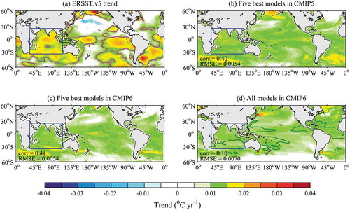
Figure 1. Spatial distribution of the SST trend in the global region during 1950–2005 (shading; units: °C yr⁻¹): (a) ERSST.v5 dataset (purple contour is the area that passes the 95% confidence test of the warming trend); (b) averaged values of the top five CMIP5 models; (c) averaged values of the top five CMIP6 models; (d) composite of all CMIP6 models. The SNR (2) of the trend is indicated by the green contour for the ratio of the mean value of the trend to the standard deviation of all 37 models. The spatial correlation coefficients and RMSEs between (a) and (b–d) are respectively marked in the lower-left corner of each panel. The IO basin is indicated by the blue box (35°S–25°N, 33°–113°E)

The persistent IO warming could have impacts on climate variability over several regions. A warming trend over the IO region would not only directly modify the interannual monsoon variability (Yang et al. 2007; Swapna, Krishnan, and Wallace 2013), but also affect the water vapor transport and precipitation intensity in the monsoon region (Zhang 2001; Choudhury, Nath, and Chen 2019). Besides local responses, the regional warming in the IO also has remote effects. The warm trend in the IO has a potential impact on the positive phase shift of the North Atlantic Oscillation (Hoerling, Hurrell, and Xu 2001) and may influence El Niño events during their developing and terminating phases (Annamalai et al. 2005; Kug and Kang 2006).

Many previous studies have investigated the sustained SST warming over the IO (Levitus et al. 2000; Levitus, Antonov, and Boyer 2005; Hoerling et al. 2004; Alory, Wijffels, and Meyers 2007; Yu, Jin, and Weller 2007) and one basic reason is believed to be due to changes in net air–sea heat flux induced by global greenhouse gas concentrations, which are mainly associated with anthropogenic forcing. A few studies have suggested an important role played by ocean advection processes in warming and expansion of the Indian Ocean warm pool (Rao et al. 2012; Dong, Zhou, and Wu 2014). Investigating such half-a-century basin-wide warming relies on both observational data analysis and climate system model results. CMIP has already provided plentiful simulations, which can be used as a baseline to investigate climate variability from multiple views (Du and Xie 2008; Taylor, Stouffer, and Meehl 2012; Eyring et al. 2016; Xu, Su, and Zhu 2014; Xu et al. 2017).

However, the sustained warming phenomenon over the IO has not been analyzed based on CMIP5 and CMIP6 models yet. Therefore, this study evaluates the simulation performance of the persistent warming over the IO between CMIP5 and CMIP6 models. It is known that the climate sensitivity of some CMIP6 models is stronger than that in CMIP5 (Forster et al. 2020; Zelinka et al. 2020), due to updated parameterizations and other model changes. Such an investigation may help us validate the model simulations with observed datasets to better estimate the model uncertainty and provide some suggestions for model improvement.

2. Data and methods

The ERSST.v5 dataset is used for model validation, which provides monthly data on SST with a resolution of 2.0° × 2.0° (Huang et al. 2017). To compare the simulation performances of CMIP5 and CMIP6 models with respect to the salient warming over the IO, the outputs of the historical simulations by the available 37 CMIP5 models and 37 CMIP6 models are used here. The monthly-mean SSTs from the CMIP5 and CMIP6 models are provided by the Program for Climate Model Diagnosis and Intercomparison (Taylor, Stouffer, and Meehl 2012; Eyring et al. 2016).

Since the historical simulations in CMIP5 models are limited to 2005, the period selected in the study is 1950–2005. Comparing the trend distribution of global SST between 1950–2005 and 1950–2014, it shows that similar warming patterns occurred in these two periods (Figure 1(a) and Figure S1). All model products were remapped onto 1° × 1° grids, and the ERSST.v5 data were also remapped onto the same 1° × 1° grid for the following analysis. All the data were temporally averaged with a seven-year moving window to filter out the impact of interannual variability on the calculation results. The global region in the study is defined as (60°S–60°N, 0°–360°E), and the IO region as (35°S–25°N, 33°E–113°E).

To assess the models’ performances with respect to IO salient warming, six metrics were defined here: (1) the warming trend in the IO to assess the sustained IO warming (IO trend metric); (2) the difference in warming trends between the IO and other ocean regions to evaluate whether the warming in the IO is the most salient (Diff trend metric); (3) the correlation coefficients between the SST trends in the IO of each model and the observed data to assess the spatial similarity of SST trends (Corr IO metric); (4) the correlation coefficients between the global SST trends of each model and the observed data (Corr glb metric); (5) the root-mean-square errors (RMSEs) between the SST trends in the IO of each model and the observed data to evaluate the differences between model values and the observed values (RMSE IO metric); (6) the RMSEs between the global SST trends of each model and the observed data to evaluate the differences between model values and the observed values (RMSE glb metric).

For each metric $m$ and each model $i$, the absolute value of the error compared to observed data ($e\mathrm{i}$) is calculated, which is normalized by the CMIP5 and CMIP6 intermodel standard deviation ($\sigma \mathrm{C}\mathrm{M}\mathrm{I}\mathrm{P}5+\mathrm{C}\mathrm{M}\mathrm{I}\mathrm{P}6$) following (Bellenger et al. 2014)

(1) $e_{\mathrm{i}}=\frac{\left|m_{\mathrm{i}}-m{ }_{\mathrm{r}\mathrm{e}\mathrm{f}}\right|}{{\sigma }_{\mathrm{C}\mathrm{M}\mathrm{I}\mathrm{P}5+\mathrm{C}\mathrm{M}\mathrm{I}\mathrm{P}6}}$(1)

where $m_{\mathrm{r}\mathrm{e}\mathrm{f}}$ indicates the observed value in the first and second metric (IO trend metric and Diff trend metric), and $m_{\mathrm{r}\mathrm{e}\mathrm{f}}$ indicates the maximum correlation coefficient values of CMIP5 and CMIP6 in the two correlation metrics (Corr IO and Corr glb) and the minimum RMSE values of CMIP5 and CMIP6 in the two RMSE metrics (RMSE IO and RMSE glb).

An overall performance score is then defined as the average of these normalized errors. The lower score values correspond to better performance in representing the salient IO warming pattern by the model.

3. Results

3.1. Salient warming trends in the IO

The observed SST has undergone general warming across the global oceans since the 1950s. However, the salient warming is mainly located in the entire IO region, with a warming trend of about 0.014°C yr⁻¹ during the period 1950–2005 (Figure 1(a)). Outside of the IO region, the warming trend is generally weak, with a mean value of 0.0102°C yr⁻¹. Hence, the difference in the warming trend between the IO and other regions is 0.0038°C yr⁻¹. Similar results can also be obtained based on other observed SST datasets (Figures S2 and S3). It should be noted that some patches with significant warming can be found in other regions outside of the IO (e.g., southwestern Atlantic, eastern Pacific). However, those locally small warming regions outside of the IO are sensitive to the datasets and have little impact in the following calculation.

In the CMIP simulation results, the warming trend can be found over the global oceans (Figure 1(d)). However, the spatial distribution of the warming trend in CMIP results shows apparent differences compared with the observed pattern. The mean value of the warming trend in the IO region simulated by all CMIP6 models is 0.006°C yr⁻¹, weaker than the observed values. The simulated warming trend outside of the IO region is also weaker (0.004°C yr⁻¹). Hence, the difference in the warming trend between the IO and the outside regions in the CMIP6 results is smaller than the observed values. Similar results are also obtained based on CMIP5 (Figure S4). The simulation uncertainty between the CMIP models can be informed by the signal-to-noise ratio (SNR). The high SNR (above 2) in the IO region indicates that the salient IO warming can be captured by most CMIP models (Figure 1(d) and Figure S4).

According to the metrics mentioned above, the simulation of the salient IO warming is evaluated. Based on the score calculated by Equation (1)(1) $e_{\mathrm{i}}=\frac{\left|m_{\mathrm{i}}-m{ }_{\mathrm{r}\mathrm{e}\mathrm{f}}\right|}{{\sigma }_{\mathrm{C}\mathrm{M}\mathrm{I}\mathrm{P}5+\mathrm{C}\mathrm{M}\mathrm{I}\mathrm{P}6}}$(1) , five best models are selected from the CMIP5 models (GISS-E2-H-CC, CESM1-WACCM, GFDL-ESM2G, FIO-ESM, GISS-E2-H) (Figure 1(b)) and five best ones from the CMIP6 models (MCM-UA-1-0, CIESM, GISS-E2-1-G, FGOALS-f3-L, MPI-ESM1-2-LR) (Figure 1(c)), respectively. Comparing the SST trend distribution in Figure 1, it is found that the spatial average trend over the IO region simulated by the five best models in CMIP5 is 0.011°C yr⁻¹, and the averaged value in CMIP6 is 0.01°C yr⁻¹. Although the value of the IO warming trend simulated by CMIP5 is closer to the observed one, the distribution of CMIP5 models does not show the weak warming in the North Pacific, South Pacific, and North Atlantic.

3.2. Performance of CMIP models with respect to IO warming

The ability of the CMIP models to simulate the IO warming can be further evaluated by the defined metrics. First, the simulated values of the warming IO trend are compared with the observed trend (Figure 2(a,c)). There are several models in CMIP5 whose warming trends (IO trend metric) are quite close to the observed value (0.014°C yr⁻¹); namely, MPI-ESM-LR, CESM1-WACCM, CMCC-CMS, FGOALS-g2, NorESM1-M, CCSM4, and bcc-csm1-1-m. The difference between these seven models and the observed trend is less than 0.001°C yr⁻¹, indicating that the value of the IO warming trend is simulated well by those models. However, the difference between the trend in the IO and other ocean regions (Diff trend metric) indicates a large deviation in the simulations of almost all the CMIP5 models, and only MPI-ESM-LR, FGOALS-g2, and GFDL-ESM2M show a value relatively close to observed data (0.0038°C yr⁻¹). Particularly, there are still some models in CMIP5 where the warming trends are negative, which would reduce the overall simulation performance of CMIP5.

Figure 2. (a) Spatially averaged warming trend in the IO region of the ERSST.v5 dataset and each CMIP5 model. (b) As in (a) but for CMIP6 models. (c) Difference between the spatially averaged warming trend in the IO region and other ocean regions of the ERSST.v5 dataset and the CMIP5 models. (d) As in (c) but for CMIP6 models. All trends have units of °C yr⁻¹. The warming period selected is 1950–2005

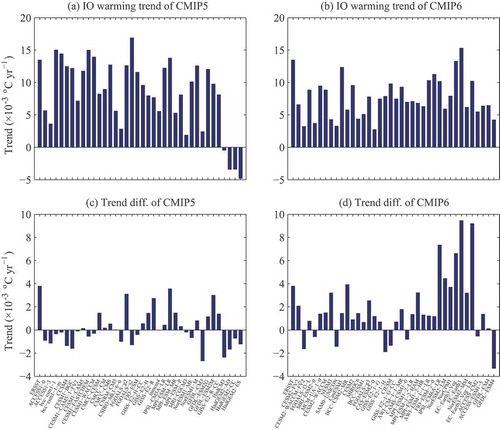
For the IO trend metric in CMIP6 (Figure 2(b)), only two models (EC-Earth3-Veg and CanESM5) have a small deviation (< 0.001°C yr⁻¹) from the observed IO warming trend. The result of this metric is not as good as CMIP5. For the metric of the difference between the trend in the IO and in other ocean regions (Diff trend metric) in CMIP6 (Figure 2(d)), six models (BCC-CSM2-MR, NorCPM1, MPI-ESM-1-2-HAM, NESM3, NorESM2-MM, and NorESM2-LM) show values close to the observed value (0.0038°C yr⁻¹). The difference between the trends in the IO and other ocean regions simulated by the models in CMIP6 is relatively better, implying a better performance in this aspect than that in CMIP5 models.

In terms of the spatial pattern of the warming trend, the RMSE and correlation coefficient metrics are used to evaluate the overall performance for the CMIP models. The RMSEs and correlation coefficients of the trends in CMIP5/CMIP6 models are calculated in the global and IO region separately (RMSE glb metric, RMSE IO metric, Corr glb metric, and Corr IO metric) (Figure 3). In the CMIP5 and the CMIP6 models, the RMSEs of the global SST trend are approximately 0.005–0.015°C yr⁻¹, which are slightly larger than those in the IO region.

Figure 3. (a) Globally averaged RMSEs of simulated warming trend relative to the observed value for each CMIP5 model. (b) As in (a) but for CMIP6 models. (c) Averaged RMSEs of simulated IO warming trend compared with observed value for each CMIP5 model. (d) As in (c) but for CMIP6 models. (e) Globally averaged correlation coefficients of the observed warming trend and the simulated value in each CMIP5 model. (f) As in (e) but for CMIP6 models. (g) Averaged correlation coefficients of the observed IO warming trend and the simulated value in each CMIP5 model. (h) As in (g) but for CMIP6 models. The units in (a–d) are °C yr⁻¹. The observed values are calculated based on the ERSST.v5 dataset. The period selected is 1950–2005

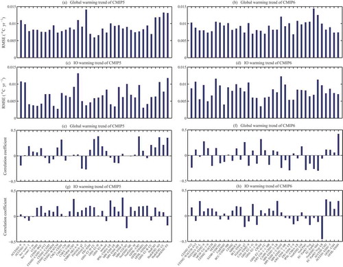
In the CMIP5 and CMIP6 models, the spatially averaged correlation coefficients of SST trends in the global region and IO region are in the range of −0.5–0.5, which indicates that most of the models in CMIP5 and CMIP6 models cannot capture the spatial pattern of the global warming well.

3.3. Simulation scores of CMIP models

To evaluate the overall performance of the CMIP models, a synthetic score is defined as the average of the above six metrics. All the metrics are ensembled together as a synthesis of the performance of each CMIP5 and CMIP6 model (Figure 4).

Figure 4. Simulation performance metrics for each model of (a) CMIP5 and (b) CMIP6. Six primary metrics are used to depict the significant warming in the IO region: IO trend (the warming trend in the IO region); Diff trend (the difference between the warming trends of the IO and other ocean regions); Corr IO (the correlation coefficients simulated by each model against the observed SST trend in the IO); Corr glb (the correlation coefficients simulated by each model against the observed SST trend in the global ocean); RMSE IO (the RMSEs simulated by each model against the observed SST trend in the IO); and RMSE glb (the RMSEs simulated by each model against the observed SST trend in the global ocean). The warming score is defined as the average of these six metrics

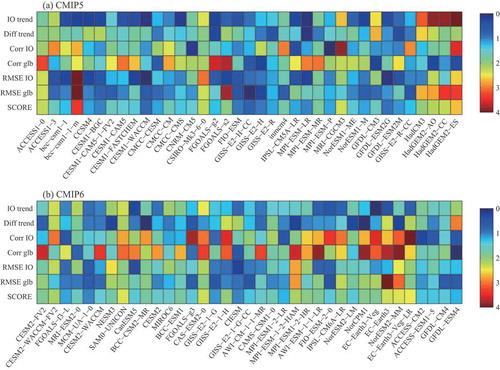
The first metric (IO trend metric) represents the difference between the trends of each model and the observed data. If the metric value is zero (the dark blue square in Figure 4), it indicates that the IO warming trend simulated by the model is the most consistent with the observed value. In contrast, a large metric value indicates that the IO warming trend simulated by this model does not match well with the observed value. Similarly, if the Diff trend metric is zero (the dark blue square in Figure 4), it indicates that the difference between the IO trend and other ocean regions simulated by this model is the most consistent with the observed value. Among the two metrics, the difference between the simulated value and the observed may be positive or negative, and its absolute value was considered here. For the correlation coefficients metrics (Corr IO metric and Corr glb metric), a zero value (the dark blue square in Figure 4) means that the correlation coefficient of the simulated trend and the observed value in this region (IO/global) is the maximum value among all models in CMIP5 and CMIP6. A larger correlation coefficient indicates a higher correlation between the simulated and observed values, suggesting a better performance of the model simulation. Similarly, if the metrics of RMSEs (RMSE IO metric and RMSE glb metric) are zero (the dark blue square in Figure 4), the RMSEs of the trends between the simulated and the observed values in this region (IO/global) are the minimum value of all RMSEs in CMIP5 and CMIP6. Smaller RMSEs indicate smaller error between the simulated and observed values, and a better performance of the model simulation.

Among all 37 models of CMIP5, there are five with the best scores (GISS-E2-H-CC, CESM1-WACCM, GFDL-ESM2G, FIO-ESM, and GISS-E2-H). The top five models are also selected among the CMIP6 models (MCM-UA-1-0, CIESM, GISS-E2-1-G, FGOALS-f3-L, and MPI-ESM1-2-LR). The scores of the top five CMIP5 models are smaller than those of the top five models in CMIP6, indicating that some models in CMIP5 have comparably higher performance in simulating the sustained warming of the IO than CMIP6 models. If being ranked according to the mean score of five metrics for all 74 models, GISS-E2-H-CC, CESM1-WACCM, and GFDL-ESM2G are the best, followed by FIO-ESM, GISS-E2-H, which are all from CMIP5. In general, however, some other models in CMIP5 also have larger errors than CMIP6. Overall, the analysis of these metrics depicts that the skills of individual models in simulating IO warming in CMIP5 are generally better than in CMIP6. However, more attention should be paid to the fact that the selected warming spatial range or other factors may affect the metric values, and further work is still needed to elucidate this finding.

4. Conclusions and discussion

Since the 1950s, the IO basin has experienced consistent warming that lasted for half a century, which may exert a profound impact on the natural environment and climate change (Han et al. 2014; Roxy et al. 2016). This study evaluated the salient warming phenomenon in the IO region simulated by 37 CMIP5 models and 37 CMIP6 models. In general, the simulated trends of the IO warming in CMIP6 models show little difference/improvement from those in CMIP5 models. Most of these models can capture the warming in the IO region, but have a tendency to underestimate the magnitude of IO warming trends, especially the CMIP6 models. Some CMIP5 models have a better representation in terms of salient warming in the IO. The differences between the IO trend and other ocean regional trends is slightly greater in CMIP6 than CMIP5 models, which indicates that the salient IO warming relative to other regions can be generally well simulated in the CMIP6 models. However, both the RMSE and correlation coefficient metrics show a better simulation performance by CMIP5 models. Regardless, there is no qualitative improvement in the simulations of the IO warming from CMIP5 to CMIP6. The cause of the better simulation of CMIP5 models has not been clarified yet. Analysis of a few studies suggests that the differences between CMIP5 and CMIP6 models may be attributable to generally greater climate sensitivity in the CMIP6 model ensemble relative to the CMIP5 ensemble (Forster et al. 2020; Zelinka et al. 2020), in part because of developments in the representation of cloud physics and the updated parameterizations. Another factor may be related with the multidecadal oscillation in the climate system, whose observed time phases can barely be well captured by current models.

It should be emphasized that the persistent IO warming is one unique phenomenon under global warming. Driven by global warming, the warming trend in any region would be irreversible sooner or later. However, the warming trend in the IO was quite salient compared with other regions during the past half-century. Besides analyses using observed datasets, investigations based on simulations/experiments with climate models could provide valuable clues for the reasons behind the persistent and significant warming in the IO. It is desirable that further research is carried out with a focus on the underlying mechanism of the sustained IO warming. To achieve such a goal, more analyses and experiments may be needed based on the climate models with a better performance for the sustained IO warming, as given based on the overall evaluation in this study.

Acknowledgments

The authors wish to thank the two anonymous reviewers for their constructive and helpful comments. The ERSST.v5 data were obtained from http://www.esrl.noaa.gov. The CMIP6 model data and CMIP5 model data are available from the ESGF at https://esgf-node.llnl.gov/search/.

Disclosure statement

No potential conflict of interest was reported by the authors.

Supplementary material

Supplemental data for this article can be accessed here.

Additional information

Funding

This work was supported by the National Key R&D Program of China [grant numbers 2016YFA0600602 and 2019YFC1510002] and the National Natural Science Foundation of China [grant number 41776039].

References

- Alory, G., S. Wijffels, and G. Meyers. 2007. “Observed Temperature Trends in the Indian Ocean over 1960–1999 and Associated Mechanisms.” Geophysical Research Letters 34 (2): L02606. doi:10.1029/2006GL028044.
- Annamalai, H., S. P. Xie, J. P. McCreary, and R. Murtugudde. 2005. “Impact of Indian Ocean Sea Surface Temperature on Developing El Niño.” Journal of Climate 18 (2): 302–319. doi:10.1175/JCLI-3268.1.
- Bellenger, H., E. Guilyardi, J. Leloup, M. Lengaigne, and J. Vialard. 2014. “ENSO Representation in Climate Models: From CMIP3 to CMIP5.” Climate Dynamics 42 (7–8): 1999–2018. doi:10.1007/s00382-013-1783-z.
- Choudhury, D., D. Nath, and W. Chen. 2019. “Impact of Indian Ocean Warming on Increasing Trend in Pre-monsoon Rainfall and Hadley Circulation over Bay of Bengal.” Theoretical and Applied Climatology 137 (3–4): 2595–2606. doi:10.1007/s00704-018-02751-2.
- Dong, L., T. J. Zhou, and B. Wu. 2014. “Indian Ocean Warming during 1958–2004 Simulated by a Climate System Model and Its Mechanism.” Climate Dynamics 42 (1–2): 203–217. doi:10.1007/s00382-013-1722-z.
- Du, Y., and S. P. Xie. 2008. “Role of Atmospheric Adjustments in the Tropical Indian Ocean Warming during the 20th Century in Climate Models.” Geophysical Research Letters 35 (8): L08712. doi:10.1029/2008GL033631.
- Eyring, V., S. Bony, G. A. Meehl, C. A. Senior, B. Stevens, R. J. Stouffer, and K. E. Taylor. 2016. “Overview of the Coupled Model Intercomparison Project Phase 6 (CMIP6) Experimental Design and Organization.” Geoscientific Model Development 9 (5): 1937–1958. doi:10.5194/gmd-9-1937-2016.
- Forster, P. M., A. C. Maycock, C. M. McKenna, and C. J. Smith. 2020. “Latest Climate Models Confirm Need for Urgent Mitigation.” Nature Climate Change 10 (1): 7–10. doi:10.1038/s41558-019-0660-0.
- Han, W., J. Vialard, M. J. McPhaden, and T. Lee. 2014. “Indian Ocean Decadal Variability: A Review.” Bulletin of the American Meteorological Society 95 (11): 1679–1703. doi:10.1175/BAMS-D-13-00028.1.
- Hoerling, M. P., J. W. Hurrell, and T. Xu. 2001. “Tropical Origins for Recent North Atlantic Climate Change.” Science 292 (5514): 90–92. doi:10.1126/science.1058582.
- Hoerling, M. P., J. W. Hurrell, T. Xu, G. T. Bates, and A. S. Philips. 2004. “Twentieth Century North Atlantic Climate Change. Part II: Understanding the Effect of Indian Ocean Warming.” Climate Dynamics 23 (3–4): 391–405. doi:10.1007/s00382-004-0433-x.
- Huang, B., P. W. Thorne, V. F. Banzon, and T. Boyer. 2017. “Extended Reconstructed Sea Surface Temperature Version 5 (Ersstv5), Upgrades, Validations, and Inter-comparisons.” Journal of Climate 30 (20): 20. doi:10.1175/JCLI-D-16-0836.1.
- Ihara, C., Y. Kushnir, and M. A. Cane. 2008. “Warming Trend of the Indian Ocean SST and Indian Ocean Dipole from 1880 to 2004.” Journal of Climate 21 (10): 2035–2046. doi:10.1175/2007JCLI1945.1.
- IPCC. 2013. Climate Change 2013: The Physical Science Basis. Contribution of Working Group I to the Fifth Assessment Report of the Intergovernmental Panel on Climate Change. Cambridge, UK and New York, USA: Cambridge University Press.
- Kug, J. S., and I. S. Kang. 2006. “Interactive Feedback between ENSO and the Indian Ocean.” Journal of Climate 19 (9): 1784–1801. doi:10.1175/JCLI3660.1.
- Levitus, S., J. Antonov, and T. Boyer. 2005. “Warming of the World Ocean, 1955–2003.” Geophysical Research Letters 32. doi:10.1029/2004GL021592.
- Levitus, S., J. Antonov, T. Boyer, and C. Stephens. 2000. “Warming of the World Ocean.” Science 287 (5461): 2225–2229. doi:10.1126/science.287.5461.2225.
- Rao, S. A., A. R. Dhakate, S. K. Saha, S. Mahapatra, H. S. Chaudhari, S. Pokhrel, and S. K. Sahu. 2012. “Why Is Indian Ocean Warming Consistently?” Climatic Change 110 (3–4): 709–719. doi:10.1007/s10584-011-0121-x.
- Roxy, M. K., K. Ritika, P. Terray, and S. Masson. 2016. “The Curious Case of Indian Ocean Warming.” Journal of Climate 27 (22): 8501–8509. doi:10.1175/JCLI-D-14-00471.1.
- Swapna, P., R. Krishnan, and J. M. Wallace. 2013. “Indian Ocean and Monsoon Coupled Interactions in a Warming Environment.” Climate Dynamics 42 (9–10): 2439–2454. doi:10.1007/s00382-013-1787-8.
- Taylor, K. E., R. J. Stouffer, and G. A. Meehl. 2012. “An Overview of CMIP5 and the Experiment Design.” Bulletin of the American Meteorological Society 93 (4): 485–498. doi:10.1175/BAMS-D-11-00094.1.
- Xu, K., J. Su, and C. Zhu. 2014. “The Natural Oscillation of Two Types of ENSO Events Based on Analyses of CMIP5 Model Control Runs.” Advances in Atmospheric Sciences 31 (4): 801–813. doi:10.1007/s00376-013-3153-5.
- Xu, K., C. Y. Tam, C. Zhu, and B. Liu. 2017. “CMIP5 Projections of Two Types of El Niño and Their Related Tropical Precipitation in the Twenty-First Century.” Journal of Climate 30 (3): 849–864. doi:10.1175/JCLI-D-16-0413.1.
- Yamagata, T., S. K. Behera, J. J. Luo, S. Masson, M. R. Jury, and S. A. Rao. 2004. “Coupled Ocean-atmosphere Variability in the Tropical Indian Ocean.” Washington Dc American Geophysical Union Geophysical Monograph 147: 189–211. doi:10.1029/147GM12.
- Yang, J., Q. Liu, S. P. Xie, Z. Liu, and L. Wu. 2007. “Impact of the Indian Ocean SST Basin Mode on the Asian Summer Monsoon.” Geophysical Research Letters 34 (2): L02708. doi:10.1029/2006GL028571.
- Yu, L., X. Jin, and R. A. Weller. 2007. “Annual, Seasonal, and Interannual Variability of Air-sea Heat Fluxes in the Indian Ocean.” Journal of Climate 20 (13): 3190–3209. doi:10.1175/JCLI4163.1.
- Zelinka, M. D., T. A. Myers, D. T. McCoy, S. Po-Chedley, P. M. Caldwell, P. Ceppi, S. A. Klein, and K. E. Taylor. 2020. “Causes of Higher Climate Sensitivity in CMIP6 Models.” Geophysical Research Letters 47 (e2019GL085782). doi:10.1029/2019GL085782.
- Zhang, R. H. 2001. “Relations of Water Vapor Transport from Indian Monsoon with that over East Asia and the Summer Rainfall in China.” Advances in Atmospheric Sciences 18 (5): 1005–1017. doi:10.1007/BF02919315.