Estimation of land surface evapotranspiration using the METRIC model in Nepal

ABSTRACT

Climatic and atmospheric properties vary significantly within a small area for a topographically diverse region like Nepal. Remote sensing can be used for large-scale monitoring of atmospheric parameters in such diverse terrains. This work evaluates the Landsat-based METRIC (Mapping Evapotranspiration at High Resolution with Internalized Calibration) model for estimating Evapotranspiration (ET) in Nepal. The slope and aspect of terrain are accounted for in our implementation, making the model suitable for regions with topographical variations. The estimations obtained from the model were compared with ground-based measurements. The root-mean-square error for hourly ET (daily ET) was 0.06 mm h⁻¹ (1.24 mm d⁻¹), while the mean bias error was 0.03 mm h⁻¹ (0.29 mm d⁻¹). These results are comparable with results from other studies in the literature that have used the METRIC model for different regions of the world. Thus, this work validates the applicability of the METRIC model for ET estimation in a mountainous area like Nepal. Further, this implementation provides ET estimation at a very high resolution of 30 m compared to the best available resolution of 5 km in earlier works, without compromising on the accuracy. ET estimation with high resolution over a large region in Nepal has applications in agricultural planning and monitoring, among others.

Graphical abstract

摘要

鉴于尼泊尔地区地形复杂, 大气和气候特性的局地性变化很强, 我们尝试将遥感用于该地区复杂地形以检测大气参数。本研究评估了基于Landsat的METRIC模型在尼泊尔地区复杂下垫面估算蒸散量的适用性, 同时也考虑了地形的坡度和坡向对模拟的影响。结果表明, 每小时ET (每日ET) 的均方根误差为0.06mm h⁻¹ (1.24mm d⁻¹), 而平均偏差误差为0.03mm h⁻¹ (0.29mm d⁻¹) 。这一结果与前人评估METRIC模型所得到的结果类似, 因此验证了该模型在尼泊尔地区的适用性。我们的研究将ET估算的分辨率提升至30m的同时不会影响其精度。在尼泊尔的复杂地形下, 高分辨率的ET估算可用于农业规划和监测等。

KEYWORDS:

• Evapotranspiration
• metric model
• Landsat 8
• elevation
• complex terrain

关键词:

• 蒸散发
• METRIC模型
• 陆地卫星8号
• 高程
• 复杂地形

1. Introduction

Evapotranspiration (ET), the phenomenon of the loss of water to the atmosphere from the land surface through evaporation and transpiration, is an important part of water and energy cycles (Jung et al. 2010). ET is a key variable used in applications such as drought monitoring, climate prediction, water resources management, and agricultural planning (Friedlingstein et al. 2014; Mancosu et al. 2015), given the role it plays in the water cycle. For example, ET estimation is used in irrigation system planning for maximized crop productions with minimum water loss (Boudhina et al. 2018).

Various surface energy balance models based on remote sensing have been developed for ET estimation over large areas (Bastiaanssen 1998; Tasumi et al. 2005a, 2005b; Allen et al. 2007), since ground-based ET measurements can only provide point estimations and cannot be scaled for large areas. For example, Ma et al. (2012) studied ET estimation in Australia with the SEBS (Surface Energy Balance System) model using Landsat-5 data. Similarly, ET estimation for regions in Saudi Arabia, South Dakota, and California has been investigated using the Landsat-based METRIC (Mapping Evapotranspiration at High Resolution with Internalized Calibration) model (Madugundu et al. 2017; Reyes-González et al. 2017; He et al. 2017). In these studies, ET estimated from remote sensing was found to agree closely with ground-based measurements. There have also been studies on remote sensing–based ET estimation in Nepal. Amatya et al. (2015) investigated the trend of land surface heat flux (the energy balance component associated with ET) in Nepal using the SEBS model and Moderate Resolution Imaging Spectroradiometer (MODIS) data. Similarly, Amatya et al. (2016) used MODIS data and the TESEBS (Topographically Enhanced Surface Energy Balance System) model to estimate land surface heat fluxes over Nepal. Both these studies employed MODIS data, which have a low spatial resolution of 5 km. However, Nepal’s topography is highly diverse, and thus a low spatial resolution of estimation might not adequately represent the local variations of ET. There are significant changes in vegetation, land-use types, and land topology within a short distance, which contribute to the differences in energy and water cycles. This, in turn, leads to possible differences in ET. As estimating ET over short distances with ground-based stations is cost-prohibitive, ET estimation with remote sensing remains the only alternative. High-resolution ET estimation in Nepal using remote sensing helps us to understand the climatic patterns and energy–water cycle balances in a region, and we can then use this understanding in irrigation planning, for example. The importance of a high-resolution ET estimation has also been highlighted for agricultural applications where site-specific monitoring is needed (Mulla 2013), which is highly relevant for a country like Nepal that relies on agriculture for the majority share of its GDP and employment workforces.

In this work, we investigated ET estimation in Nepal using Landsat-8 data. We used the METRIC model for estimation and included surface slope, aspect, and temperature lapsing in the modeling to make it applicable for both flat and mountainous terrains present in Nepal. ET estimation is obtained with a high spatial resolution of 30 m, corresponding to the Landsat-8 data resolution. We validated the model by comparing the estimated ET with ground-based measurements. We also analyzed the elevation-wise variation of ET as seen in different months across the seasons. This analysis sheds further light on the impact of topography and land surface properties on ET. To the best of our knowledge, our study is the first to investigate ET estimation over a topographically diverse region like Nepal with the fine spatial resolution afforded by Landsat. Such large-scale ET estimation in Nepal has applications in agricultural planning and forecasting, among others.

2. Methods and data

2.1. Study area

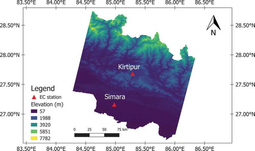
The study area considered for our work was the central part of Nepal, located over (26.54°–29.06°N, 84.14°–86.75°E) and extending from 57 m to 7782 m MSL. The study area, with the location of the eddy covariance (EC) station used for our work, is shown in Figure 1. Elevation increases in general from south to north and the land type varies with the change in elevation. There are four seasons in our considered region based on the monsoon circulation pattern: pre-monsoon (March–May); monsoon (June–September); post-monsoon (October, November); and winter (December–February) (Nayava 1980).

Figure 1. Study area with the locations of the EC stations considered for our ET calculations. The color map shows the elevation distribution. We considered a region extending fully from north to south across the whole of Nepal so that the full extent of the possible elevation distribution would be included

2.2. Data

2.2.1. Remote sensing data

All the satellite-based data used in this research were downloaded from the USGS official website (https://earthexplorer.usgs.gov/). We used the Landsat-8 images from the year 2016 for our analysis, details of which are available in the Landsat-8 Data Users Handbook, 2016 (https://landsat.usgs.gov/landsat-8-l8-data-users-handbook). Landsat-8 has two sensors onboard: the Operational Land Imager (OLI) and Thermal Infrared Sensor (TIRS). Bands 2, 4, 5, 6, and 7 from OLI and band 10 from TIRS were used in our work. The path, row, and satellite overpass date of Landsat-8 for our study area are given in Table 1. For these dates and areas, the images had less than 10% cloud cover.

Table 1. Paths, rows, and dates of satellite overpass of Landsat-8 for our study area. Two Landsat-8 tiles cover the whole study area that we considered. We considered six different days to capture possible seasonal variations in our analysis

Paths	Rows	Dates of satellite overpass
141	41	15 March 2016 April, 18 May, 3 June 2025 October, 10 November 2016
141	40	15 March 2016 April, 18 May, 3 June 2025 October, 10 November 2016

The METRIC model requires a land-use map and digital elevation information of the selected area. We obtained the land-use map from the International Center for Integrated Mountain Development (Uddin et al. 2015) and the digital elevation model (DEM) from the Advanced Spaceborne Thermal Emission Reflectance Radiometer Global Digital Elevation Model (NASA/METI/AIST/Japan Spacesystems 2019).

2.2.2. Meteorological data

We used the data from the EC flux towers (established by cooperation between the Institute of Tibetan Plateau Research, Chinese Academy of Sciences, and Tribhuvan University) at two station locations (Kirtipur and Simara) in Nepal, as a ground-based meteorological data reference. The elevation, latitude, and longitude of these stations are given in Table 2. Both Kirtipur and Simara stations are situated in a grassland area. Meteorological measurements at these stations are obtained with sensors installed at a 40-m planetary boundary layer tower. Wind speed and near-surface vapor pressure from Kirtipur station (used for model calibration) were employed for the computation of reference sensible heat flux. Besides these, air temperature, soil heat flux, net radiation, hourly wind speed at 2 m, and the saturation and actual vapor pressure (kPa) measured by the station were used for the calculation of the reference ET in the model calibration. Similar meteorological parameters from Simara station were used to compute the ET for validation. For obtaining relevant information for a study area, e.g., identifying the estimated ET for the station area, an average of the estimations available within and surrounding an area (if no estimations are available in the region, e.g., due to cloud) can be used. Details about the station data measurements and processing to derive different heat fluxes and ET can be found in the work of Joshi et al. (2020).

Table 2. Locations of the EC flux tower site measurements of the two different stations

Location	Elevation (MSL)	Latitude	Longitude
Simara	137	27.16°N	84.98°E
Kirtipur	1318	27.68°N	85.29°E

2.3. Landsat data preprocessing

Landsat-8 Collection-1 level-1 images are in the form of a quantized digital number (DN). This DN was converted to at-sensor radiance and top-of-the-atmosphere (TOA) reflectance, with a correction for solar zenith angle as:

(1) ${\mathrm{L}}_{\lambda }=\mathrm{M}\mathrm{L}\times Q_{\mathrm{c}\mathrm{a}\mathrm{l}}+\mathrm{A}\mathrm{L},$(1)

where $L_{\lambda }$ is TOA radiance without correction for the solar angle (W m⁻²× srad⁻¹× μm⁻¹), ML is a band-specific multiplicative rescaling factor, AL is a band-specific additive rescaling factor, and $Q_{\mathrm{c}\mathrm{a}\mathrm{l}}$ is DN. DN was converted to TOA reflectance without correction for solar angle as:

(2) $\begin{array}{c}{{\rho }^{\prime }}_{\lambda }=M_{\rho }\times Q_{\mathrm{c}\mathrm{a}\mathrm{l}}+A_{\rho },\end{array}$(2)

where ${\rho }_{\lambda }^{\prime }$ is TOA reflectance without correction for the solar angle, $M_{\rho }$ is a band-specific multiplicative rescaling factor, and $A_{\rho }$ is a band-specific additive rescaling factor.

The TOA reflectance with correction for solar zenith angle was then obtained with:

(3) $\begin{array}{c}{\rho }_{\lambda }=\frac{{{\rho }^{\prime }}_{\lambda }}{\mathrm{c}\mathrm{o}\mathrm{s}{\theta }_{\mathrm{S}\mathrm{Z}\mathrm{A}}},\end{array}$(3)

where θ_SZA is the solar zenith angle.

2.4. METRIC model

METRIC is a surface energy balance model for estimating ET over diverse terrains (Allen, Tasumi, and Trezza 2007). ET is estimated from the energy balance equation given as:

(4) $\begin{array}{c}\mathrm{L}\mathrm{E}=R_{\mathrm{n}}-G-H,\end{array}$(4)

where R_n is the net radiation (W m⁻²), G is the soil heat flux (W m⁻²), H is the sensible heat flux (W m⁻²), and LE is the latent heat flux (W m⁻²) associated with ET.

To compute R_n, outgoing radiant fluxes are subtracted from incoming radiant fluxes:

(5) $\begin{array}{c}{R}_{\mathrm{n}}=R_{\mathrm{S}\downarrow }-\alpha R_{\mathrm{S}\downarrow }+R_{\mathrm{L}\downarrow }-R_{\mathrm{L}\uparrow }-\left(1-{\epsilon }_{\mathrm{o}}\right)\times R_{\mathrm{L}\downarrow },\end{array}$(5)

where R_S↓ and R_L↓ are incoming broadband shortwave radiation and longwave radiation, respectively; R_L↑ is the outgoing longwave radiation; εₒ is broadband surface thermal emissivity, and α is surface albedo. The slope and aspect of the terrain are also accounted for when computing R_S↓, R_L↓, and R_L↑, similar to the work of Allen, Tasumi, and Trezza (2007). εₒ and α were computed according to Tasumi (2003) and Naegeli et al. (2017), respectively.

The land surface temperature (LST), required in the METRIC model, was computed as in Stathopoulou and Cartalis (2007):

(6) $\begin{array}{c}{T}_{\mathrm{s}}=\frac{\mathrm{T}\mathrm{B}}{\left[1+\left\{\left(\frac{\lambda \mathrm{T}\mathrm{B}}{\text{Deltaa}}\right)\mathrm{l}\mathrm{n}{\epsilon }_{\lambda }\right\}\right]}+273.15,\end{array}$(6)

where T_s is the LST (K), λ is the average wavelength of a given band, and ƍ$=h\times \frac{c}{\sigma }$, in which σ, h, and c are the Boltzmann constant, Plank’s constant, and the speed of light. The emissivity ε_λ was computed as per Sobrino, Jiménez-Muñoz, and Paolini (2004). TB is the brightness temperature, obtained using TIRS band-10 data, as per the Landsat-8 product guide (http://landsat.usgs.gov/Landsat8).

The soil heat flux, G, in the energy balance equation was calculated using an empirical equation developed by Tasumi (2003):

(7) $\begin{array}{c}\frac{G}{R_{\mathrm{n}}}=0.05+0.18{\mathrm{e}}^{-0.521\mathrm{L}\mathrm{A}\mathrm{I}}\left(\mathrm{L}\mathrm{A}\mathrm{I}\ge 0.5\right);\end{array}$(7)

(8) $\begin{array}{c}\frac{G}{R_{\mathrm{n}}}=\frac{1.80\left(T_{\mathrm{s}}-273.15\right)}{R_{\mathrm{n}}}+0.084\left(\mathrm{L}\mathrm{A}\mathrm{I}<0.5\right),\end{array}$(8)

where T_s is the surface temperature (K) and LAI is the leaf area index computed as in Bastiaanssen (1998).

H was computed as a function of aerodynamic resistance as:

(9) $\begin{array}{c}H={\rho }_{\mathrm{a}\mathrm{i}\mathrm{r}}{C}_p\frac{\mathrm{d}T}{r_{\mathrm{a}\mathrm{h}}},\end{array}$(9)

where ${\rho }_{\mathrm{a}\mathrm{i}\mathrm{r}}$ is the air density (kg m⁻³) computed as in Allen et al. (1998), C_p is the specific heat of air at constant pressure, dT represents the temperature difference between two heights (z₁ and z₂) in a near-surface blended area (K), and r_ah is the aerodynamic resistance (s m⁻¹) between these heights.

The dT, required for computing H, was obtained as a linear function of surface temperature T_{s datum} as per Bastiaanssen and Maria (1995):

(10) $\begin{array}{c}\mathrm{d}T=a\times T_{\mathrm{s}\mathrm{d}\mathrm{a}\mathrm{t}\mathrm{u}\mathrm{m}}+b,\end{array}$(10)

where a and b are constants for a satellite image. T_{s datum} is adjusted based on the DEM and a fixed lapse rate to account for elevation. The constants of the linear equation were computed using ‘hot’ and ‘cold’ anchor pixels information for each satellite image, similar to Allen, Tasumi, and Trezza (2007). Hot and cold pixels were computed automatically in our work using the land-use map and LST. The r_ah, required for computing H, was obtained as in Allen, Tasumi, and Trezza (2007):

(11) $\begin{array}{c}{r}_{\mathrm{a}\mathrm{h}}=\frac{\left(ln\frac{z_2}{z_1}\right)}{u^{\ast }\times k},\end{array}$(11)

where z₁ and z₂ are the same heights used for the definition of dT, k is von Karman’s constant, and $u^{\ast }=\frac{k{u}_{200}}{ln\left(\frac{200}{z_{\mathrm{o}\mathrm{m}}}\right)}$ is friction velocity (m s⁻¹), in which u₂₀₀ is the wind speed at a blending height of 200 m (m s⁻¹), and z_om is the momentum roughness length (m). The z_om was computed as a function of LAI as in Tasumi (2003) for agricultural areas. For non-agricultural areas, z_om is known and was assigned using the land-use map. We computed z_om pixel-wise by considering the slope as in Tasumi (2003). The height of 200 m is considered as a blending height in the METRIC model. The corresponding wind speed at this height was computed as:

(12) $\begin{array}{c}{u}_{200}=\frac{u_{\mathrm{w}}ln\left(\frac{200}{z_{\mathrm{o}\mathrm{m}\mathrm{w}}}\right)}{ln\left(\frac{z_x}{z_{\mathrm{o}\mathrm{m}\mathrm{w}}}\right)},\end{array}$(12)

where u_w is the wind speed as registered in the weather station at z_x height, and z_omw is the weather station area’s roughness length computed as in Brutsaert (1982). The value of u₂₀₀ was further adapted considering the wind speed weighting coefficient as in Tasumi (2003).

ET (which is then corresponding to the time of the image taken by the satellite) was finally computed for each pixel with:

(13) $\begin{array}{c}\mathrm{E}{\mathrm{T}}_{\mathrm{i}\mathrm{n}\mathrm{s}\mathrm{t}}=3,600\frac{\mathrm{L}\mathrm{E}}{1{\rho }_{\mathrm{w}}},\end{array}$(13)

where ET_inst is instantaneous ET (mm h⁻¹) and ${\rho }_{\mathrm{w}}$ and λ1 are the values of water density and latent heat of vaporization (J kg⁻¹), respectively.

After the computation of ET_inst, the reference evapotranspiration fraction (ET_rF) was computed for each pixel with:

(14) $\begin{array}{c}\mathrm{E}{\mathrm{T}}_{\mathrm{r}}F=\frac{\mathrm{E}{\mathrm{T}}_{\mathrm{i}\mathrm{n}\mathrm{s}\mathrm{t}}}{\mathrm{E}{\mathrm{T}}_{\mathrm{r}}},\end{array}$(14)

where ET_inst, ET_r, and ET_rF are in mm h⁻¹. ET_r, the reference ET from station data, was computed using the ASCE Penman–Monteith method (Allen et al. 2005).

Daily ET could be more useful than the instantaneous ET. So, for each pixel of the image, daily ET was computed from ET_rF and 24-h ET_r as:

(15) $\begin{array}{c}\mathrm{E}{\mathrm{T}}_{24}=\mathrm{E}{\mathrm{T}}_{\mathrm{r}}F\times \mathrm{E}{\mathrm{T}}_{\mathrm{r}-24},\end{array}$(15)

where ET₂₄ is the daily actual ET (mm d⁻¹) and ET_r-24 is the 24-h ET_r computed from weather station data.

2.4.1. Error estimation

We validated T_s and ET estimated from the METRIC model using measurements from the EC flux tower at the validation site of Simara, with root-mean-square error (RMSE) and mean bias error (MBE) computed as:

(16) $\begin{array}{c}\mathrm{R}\mathrm{M}\mathrm{S}\mathrm{E}=\sqrt{\frac{{\sum }_{i=1}^n{\left(\mathrm{M}\mathrm{E}\mathrm{T}\mathrm{R}\mathrm{I}\mathrm{C}\mathrm{E}\mathrm{T}-\mathrm{f}\mathrm{l}\mathrm{u}\mathrm{x}\mathrm{t}\mathrm{o}\mathrm{w}\mathrm{e}\mathrm{r}\mathrm{E}\mathrm{T}\right)}^2}{n}};\end{array}$(16)

(17) $\begin{array}{c}\mathrm{M}\mathrm{B}\mathrm{E}=\frac{{\sum }_{i=1}^n\left(\mathrm{f}\mathrm{l}\mathrm{u}\mathrm{x}\mathrm{t}\mathrm{o}\mathrm{w}\mathrm{e}\mathrm{r}\mathrm{E}\mathrm{T}-\mathrm{M}\mathrm{E}\mathrm{T}\mathrm{R}\mathrm{I}\mathrm{C}\mathrm{E}\mathrm{T}\right)}{n},\end{array}$(17)

where n is the number of samples taken.

3. Results

3.1. Hourly and daily ET derived from the METRIC model

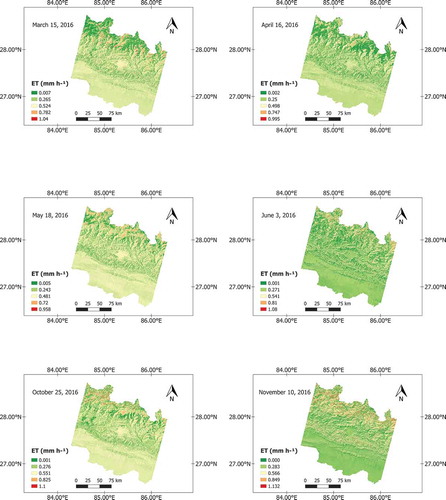
We computed the hourly and daily ET for different months using the METRIC model. T_s, vegetation indices (NDVI, SAVI, and LAI), surface albedo, and heat fluxes were all computed as intermediate products in the model. The average values for these parameters for different months are given in Table 3. The average ET_inst obtained from the METRIC model for the months of March, April, May, June, October, and November was 0.36, 0.28, 0.35, 0.26, 0.39, and 0.31 mm h⁻¹, respectively. Similarly, the daily ET obtained was 4.33, 7.009, 4.29, 3.24, 3.97, and 1.5 mm d⁻¹, respectively. The estimated ET at the time of satellite overpass for different months in our study area is shown in Figure 2.

Table 3. METRIC-derived intermediate products for the months of March, April, May, June, October, and November 2016

Month	Average Ts (°C)	Average NDVI	Average Rn (W m^−2)	Average G (W m^−2)	Average H (W m^−2)	Average LE (W m^−2)
March	19.1	0.36	610.83	92.13	292.56	226.11
April	23.62	0.21	608.86	94.23	345.75	168.66
May	24.48	0.41	655.75	100.74	326.28	228.73
June	22.12	0.34	353.73	59.64	166.57	127.05
October	20.72	0.51	680.62	91.21	336.92	249.91
November	20.48	0.52	420.59	60.15	200.76	157.39

Figure 2. METRIC-derived ET at the time of satellite overpass for 15 March 2016 (upper left), 16 April 2016 (upper right), 18 May 2016 (middle left), 3 June 2016 (middle right), 25 October 2016 (lower left), and 10 November 2016 (lower right)

3.2. Validation of the METRIC-derived ET and T_s

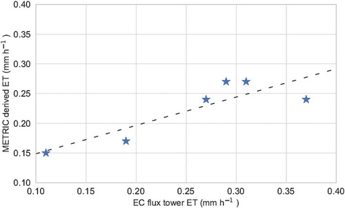
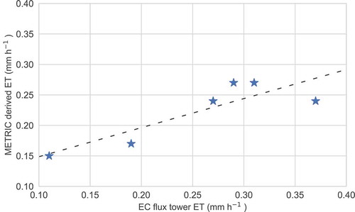
The METRIC-derived ET and T_s were found to be in close agreement with the flux tower–based ET and T_s measurements. These results are shown with a scatterplot in Figure 3. The RMSE for hourly ET and daily ET was 0.06 mm h⁻¹ and 1.24 mm d⁻¹, respectively. Similarly, the MBE for hourly and daily ET was 0.03 mm h⁻¹ and 0.29 mm d⁻¹, respectively. The RMSE and MBE for T_s was 4.93°C and −0.49°C, respectively. We obtained a mean absolute percentage error of 35.07% for LE estimation, where the mean absolute percentage error is the percentage ratio of the absolute error in estimation to the reference value. We computed this metric to compare our validation results with earlier works on LE estimation for Nepal.

Figure 3. ET estimated from the METRIC model in comparison to the ET from the flux tower from Simara across different months

3.3. Elevation-wise variation in ET

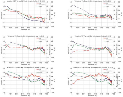
Based on the results obtained for our study area (shown in Figure 2), elevation-wise variations in ET, T_s, and NDVI for six different months were obtained and are shown in Figure 4. We averaged the values within a given height, with a resolution for the height of 10 m, to obtain the relation. The obtained curve was further smoothed with cubic spline interpolation. In March, April, and May, the maximum ET was 0.42, 0.33, and 0.41 mm h⁻¹, respectively. Similarly, the minimum ET was 0.07, 0.14, and 0.13 mm h⁻¹, respectively. In March, April, and May, the maximum ET was seen at lower elevations between 57 m and 300 m, and the minimum ET was seen above 6000 m. For June, October, and November, at lower elevations below 300 m, the estimated ET was 0.26, 0.47, and 0.24 mm h⁻¹, respectively. The maximum ET obtained for June, October, and November was 0.36, 0.48, and 0.49 mm h⁻¹, and the minimum ET was 0.09, 0.13, and 0.12 mm h⁻¹, respectively. T_s and NDVI were also seen to be high in the lower elevations and low in the higher elevations.

Figure 4. Variation of ET, T_s, and NDVI with elevation for 15 March 2016 (upper left), 16 April 2016 (upper right), 18 May 2016 (middle left), 3 June 2016 (middle right), 25 October 2016 (lower left), and 10 November 2016 (lower right)

4. Discussion

We validated the results of T_s and ET estimation from the METRIC model with the EC station data from Simara, an independent validation site. METRIC model estimations were in close agreement with the EC station measurements. We obtained an RMSE of 0.06 mm h⁻¹ and 1.24 mm d⁻¹ for ET estimation. This is comparable with evaluations of the METRIC model in other regions of the world (Madugundu et al. 2017; Reyes-González et al. 2017; He et al. 2017). Thus, the METRIC model is applicable for a topographically diverse region like Nepal, likely because terrain properties are accounted for in the model. The state-of-the-art on remote sensing–based LE estimation for Nepal reported a mean percentage error of 36.01% (Amatya et al. 2015) with the model output resolution of 5 km. In comparison, we obtained a comparable accuracy (35.07%) while providing a much higher resolution (30 m).

We analyzed the elevation-wise variations of ET, T_s, and NDVI for different months (Figure 4). ET decreased as the elevation increased in March, April, and May, likely due to the decreasing T_s and NDVI. In the land-use map of our study area (Uddin et al. 2015), lower elevations are mostly composed of irrigated agricultural areas and higher elevations of barren areas and snow/glaciers. This further supports the observed effect of decreasing ET with increasing elevation. However, ET is also a complex parameter that depends on several other factors such as wind speed and land terrain properties, besides NDVI and T_s. We observed some aberrations in the general trend of elevation-wise variations of ET—for example, in some elevation ranges for November (Figure 4). One likely explanation for ET not decreasing with elevation is because the T_s and NDVI do not decrease as sharply in this month, and other parameters that affect ET could have dwarfed the effect of T_s and NDVI on ET. This will be further studied in future work.

5. Conclusions

Topographically diverse regions like Nepal require ET estimation with high spatial resolution, given the lack of ground station infrastructures to monitor large areas. In this work, we evaluated a remote sensing–based ET estimation using the METRIC model and high-resolution Landsat-8 data. The ET and T_s estimated from the model were found to be in close agreement with the ground-based measurements. Thus, we conclude that the METRIC model is suitable for a region like Nepal with high topographical diversity. Compared to previous works on ET estimation in Nepal with the best resolution of 5 km, our model estimates have a resolution of 30 m. Such high-resolution ET estimation is essential for agricultural planning and monitoring applications. We also validated the direct effect that T_s and vegetation have on ET, in the context of Nepal, by studying the elevation-wise variations of ET. Seasonal variations in the elevation-wise profile of ET are apparent based on our analysis, which has implications for applications such as irrigation projects.

Acknowledgments

The authors are grateful for the open-source data provided by the USGS.

Disclosure statement

The authors declare no conflict of interest.

Additional information

Funding

This research was funded by the Second Tibetan Plateau Scientific Expedition and Research Program [grant number 2019QZKK0103], the Strategic Priority Research Program of the Chinese Academy of Sciences [grant number XDA20060101], and the National Natural Science Foundation of China [grant numbers 41830650, 91737205, and 91837208].

References

- Allen, R. G., I. A. Walter, R. Elliot, T. Howell, D. Itenfisu, and M. Jensen. 2005. “The ASCE Standardized Reference Evapotranspiration Equation.” ASCE-EWRI Task Committee Final Report.
- Allen, R. G., L. S. Pereira, D. Raes, and M. Smith. 1998. “Crop evapotranspiration-Guidelines for Computing Crop Water requirements-FAO Irrigation and Drainage Paper 56.” Fao, Rome 300 (9): D05109.
- Allen, R. G., M. Tasumi, A. Morse, R. Trezza, J. L. Wright, W. Bastiaanssen, W. Kramber, I. Lorite, and C. W. Robison. 2007. “Satellite-based Energy Balance for Mapping Evapotranspiration with Internalized Calibration (Metric)—applications.” Journal of Irrigation and Drainage Engineering 133 (4): 395–406. doi:10.1061/(ASCE)0733-9437(2007)133:4(395).
- Allen, R. G., M. Tasumi, and R. Trezza. 2007. “Satellite-based Energy Balance for Mapping Evapotranspiration with Internalized Calibration (Metric)—model.” Journal of Irrigation and Drainage Engineering 133 (4): 380–394. doi:10.1061/(ASCE)0733-9437(2007)133:4(380).
- Amatya, P. M., M. Yaoming, C. Han, B. Wang, and L. P. Devkota. 2015. “Recent Trends (2003–2013) of Land Surface Heat Fluxes on the Southern Side of the Central Himalayas, Nepal.” Journal of Geophysical Research: Atmospheres 120 (23): 11957–11970.
- Amatya, P. M., M. Yaoming, C. Han, B. Wang, and L. P. Devkota. 2016. “Mapping Regional Distribution of Land Surface Heat Fluxes on the Southern Side of the Central Himalayas Using TESEBS.” Theoretical and Applied Climatology 124 (3–4): 835–846. doi:10.1007/s00704-015-1466-2.
- Bastiaanssen, W. G. M. 1995. “Regionalization of Surface Flux Densities and Moisture Indicators in Composite Terrain: A Remote Sensing Approach under Clear Skies in Mediterranean Climates.” PhD diss., Wageningen Agricultural University.
- Bastiaanssen, W. G. M. 1998. Remote Sensing in Water Resources Management: State of the Art. Colombo: International Water Management Institute.
- Boudhina, N., M. M. Masmoudi, F. Jacob, L. Prévot, R. Zitouna-Chebbi, I. Mekki, and N. B. Mechlia. 2018. “Measuring Crop Evapotranspiration Over Hilly Areas”. Euro-Mediterranean Conference for Environmental Integration, Sousse, Tunisia, 22-25 November 2017.
- Brutsaert, W. 1982. Evaporation into the Atmosphere: Theory, History, and Applications. Dordrecht: Springer.
- Friedlingstein, P., M. Meinshausen, V. K. Arora, C. D. Jones, A. Anav, S. K. Liddicoat, and R. Knutti. 2014. “Uncertainties in CMIP5 Climate Projections Due to Carbon Cycle Feedbacks.” Journal of Climate 27 (2): 511–526. doi:10.1175/JCLI-D-12-00579.1.
- He, R., Y. Jin, M. M. Kandelous, D. Zaccaria, B. L. Sanden, R. L. Snyder, J. Jiang, and J. W. Hopmans. 2017. “Evapotranspiration Estimate over an Almond Orchard Using Landsat Satellite Observations.” Remote Sensing 9 (5): 436.
- Joshi, B. B., M. Yaoming, M. Weiqiang, M. Sigdel, B. Wang, and S. Subba. 2020. “Seasonal and Diurnal Variations of Carbon Dioxide and Energy Fluxes over Three Land Cover Types of Nepal.” Theoretical and Applied Climatology 139 (1–2): 415–430. doi:10.1007/s00704-019-02986-7.
- Jung, M., M. Reichstein, P. Ciais, S. I. Seneviratne, J. Sheffield, M. L. Goulden, G. Bonan, A. Cescatti, J. Chen, and R. De Jeu. 2010. “Recent Decline in the Global Land Evapotranspiration Trend Due to Limited Moisture Supply.” Nature 467 (7318): 951.
- Ma, W., M. Hafeez, U. Rabbani, H. Ishikawa, and M. Yaoming. 2012. “Retrieved Actual ET Using SEBS Model from Landsat-5 TM Data for Irrigation Area of Australia.” Atmospheric Environment 59: 408–414. doi:10.1016/j.atmosenv.2012.05.040.
- Madugundu, R., K. A. Al-Gaadi, E. Tola, A. A. Hassaballa, and V. C. Patil. 2017. “Performance of the METRIC Model in Estimating Evapotranspiration Fluxes over an Irrigated Field in Saudi Arabia Using Landsat-8 Images.” Hydrology and Earth System Sciences 21 (12): 6135–6151. doi:10.5194/hess-21-6135-2017.
- Mancosu, N., R. L. Snyder, G. Kyriakakis, and D. Spano. 2015. “Water Scarcity and Future Challenges for Food Production.” Water 7 (3): 975–992. doi:10.3390/w7030975.
- Mulla, D. J. 2013. “Twenty Five Years of Remote Sensing in Precision Agriculture: Key Advances and Remaining Knowledge Gaps.” Biosystems Engineering 114 (4): 358–371. doi:10.1016/j.biosystemseng.2012.08.009.
- Naegeli, K., A. Damm, M. Huss, H. Wulf, M. Schaepman, and M. Hoelzle. 2017. “Cross-Comparison of Albedo Products for Glacier Surfaces Derived from Airborne and Satellite (Sentinel-2 and Landsat 8) Optical Data.” Remote Sensing 9 (2): 110. doi:10.3390/rs9020110.
- NASA/METI/AIST/Japan Spacesystems, and U.S./Japan ASTER Science Team. 2019. “ASTER Global Digital Elevation Model V003.” distributed by NASA EOSDIS Land Processes DAAC. doi:10.5067/ASTER/ASTGTM.003.
- Nayava, J. L. 1980. “Rainfall in Nepal.” Himalayan Review 12: 1–18.
- Reyes-González, A., J. Kjaersgaard, T. Trooien, C. Hay, and L. Ahiablame. 2017. “Comparative Analysis of METRIC Model and Atmometer Methods for Estimating Actual Evapotranspiration.” International Journal of Agronomy 2017: 1–16. doi:10.1155/2017/3632501.
- Sobrino, J. A., J. C. Jiménez-Muñoz, and L. Paolini. 2004. “Land Surface Temperature Retrieval from LANDSAT TM 5.” Remote Sensing of Environment 90 (4): 434–440. doi:10.1016/j.rse.2004.02.003.
- Stathopoulou, M., and C. Cartalis. 2007. “Daytime Urban Heat Islands from Landsat ETM+ and Corine Land Cover Data: An Application to Major Cities in Greece.” Solar Energy 81 (3): 358–368. doi:10.1016/j.solener.2006.06.014.
- Tasumi, M. 2003. “Progress in Operational Estimation of Regional Evapotranspiration using Satellite Imagery.” PhD diss., University of Idaho.
- Tasumi, M., R. G. Allen, R. Trezza, and J. L. Wright. 2005a. “Satellite-based Energy Balance to Assess Within-population Variance of Crop Coefficient Curves.” Journal of Irrigation and Drainage Engineering 131 (1): 94–109.
- Tasumi, M., R. Trezza, Richard Allen, and James Wright. 2005b. “Operational Aspects of Satellite-based Energy Balance Models for Irrigated Crops in the Semi-arid US” Irrigation and Drainage Systems 19 (3–4): 355–376. doi:10.1007/s10795-005-8138-9.
- Uddin, K., H. L. Shrestha, M. S. R. Murthy, B. Bajracharya, B. Shrestha, H. Gilani, S. Pradhan, and B. Dangol. 2015. “Development of 2010 National Land Cover Database for the Nepal.” Journal of Environmental Management 148: 82–90. doi:10.1016/j.jenvman.2014.07.047.