Fair and efficient ride-scheduling: a preference-driven approach

ABSTRACT

Smart mobility and, in particular, automated ridesharing platforms promise efficient, safe, and sustainable modes of transportation in urban settings. To make such platforms acceptable to the end-users, it is key to capture their preferences not in a static manner (by determining a fixed route and schedule for the vehicle) but in a dynamic manner by giving the riders the chance to get involved in the routing process of an upcoming journey. To that end, this work provides a toolbox of multiagent methods that enable different forms of active preference-awareness in ridesharing services. We capture riders’ preferences (as end-users of a ridesharing service), preserve their privacy by avoiding expecting them to share preferences with other riders, and show the efficacy of the presented ridesharing algorithms using agent-based simulation and illustrating their utilitarian and fairness properties.

KEYWORDS:

• Smart mobility
• multiagent ridesharing methods
• preferences
• agent-based modelling
• AI for social good

1. Introduction

Ridesharing is a promising means towards reducing carbon emissions and mitigating climate change effects (Furuhata et al., 2013). Integrating preference-awareness into ridesharing systems enhances the satisfaction of the end-users and, in turn, allows efficiently using the spare capacity in urban transportation services (Rigas et al., 2014). However, although the potential gains are known, some traditional urban transportation systems – such as bus services – are not benefiting from ridesharing technologies. Our buses are still operating based on fixed schedules and, in the best case, use historical data on the behaviour of riders to improve their routes. However, determining routes based on data about past users does not necessarily fit how present riders want to use the service. For example, arguably, bus schedules that were generated based on travellers’ behaviour in 2019 (i.e., before the COVID-19 pandemic) do not satisfy what riders want in 2024. While gathering data more frequently and then fixing a static schedule is an option, in this work, we go a step further and suggest dynamic schedules that are determined based on the preferences of the current users/riders. Doing this will allow buses to provide customised services to riders, avoid wasting resources by meeting unnecessary stations, and find compromises for pickup and drop-off locations that users see preferable.

Ridesharing can be considered a vehicle routing problem that is typically solved by optimising a given global objective function. Most studies focused on optimising operational-based objective functions (Mourad et al., 2019), which usually benefit the ridesharing service provider rather than the passengers. Optimising based on the provider’s incentives would not lead to widespread adoption of this service, as passengers’ preferences are not taken into consideration. Thus, more recently, there have been studies regarding incorporating preferences or incentives of passengers into the ridesharing problem. These studies specified constraints, such as passengers’ maximum travel distance and maximum waiting time, to ensure some level of quality service, as well as incorporating new terms in the objective function, which encapsulates the overall satisfaction of passengers (Mourad et al., 2019). However, this method does not guarantee fairness among the passengers. For example, a ridesharing system might choose route A because it minimises the total waiting time and travelling time of all passengers. However, route A might lead to a longer travel time for a subset of passengers; for the sake of minimising the overall objective function, their preferences have been neglected, such that route A results in more inconvenience to them. In principle, assuming that the ideal route needs to be optimal merely based on the characteristics of the city in an objective sense (e.g., in terms of distances), ignores how satisfied riders are in a subjective sense. In such a view, ridesharing is approached and accordingly solved as a merely technical problem with no intention to take into account the social and preferential dimensions. In view of human-centred AI techniques and the need for developing trustworthy human-AI partnerships (Ramchurn et al., 2021), we see ridesharing as an inherently sociotechnical problem and argue that the acceptance of it by society depends on its ability to capture riders’ preferences throughout the journey.

In the line of work on the application of multiagent techniques to ridesharing and the so-called autonomous mobility-on-demand systems (Zhang et al., 2015), there are attempts to optimise the efficiency of using the shared space (Agatz et al., 2012), to use ridesharing for transportation of goods and passengers (van der Tholen et al., 2021), and to analyse the environmental benefits of ridesharing (Jalali et al., 2017). In comparison to techniques that build on a snapshot of the system with resource optimisation in mind (e.g., Agatz et al. (2012); Jalali et al. (2017)) and approaches on mixed rider-goods transportation settings (e.g., van der Tholen et al. (2021)), our focus is on passenger transportation and the use of ridesharing dynamically by capturing riders’ preferences. Here, it is critical to capture the preferences of passengers for a journey, and in particular, their satisfaction concerning their asserted urgency and ideal pickup/drop-off times. Moreover, it is unrealistic to assume complete knowledge about the preferences of riders (which would allow standard optimisation techniques to be applied). Instead, riders may have reservations about sharing their preferences and these may also change given additional knowledge they gain during the generation of routes. To address these challenges, our work is the first attempt to develop a safe framework (as we do not expect riders to share information between them) for preference-aware dynamic ridesharing. Moreover, in contrast to recent work that applies voting mechanisms to decide about destinations and accordingly form like-minded coalitions of riders for a journey (e.g., in Dennisen and Müller (2016)), we focus on a given set of users (e.g., employees of a company) and work on the satisfaction of users by allowing them to participate in the planning of the journey.¹

Against this background, this is the first contribution that develops algorithms for determining ridesharing routes in participation with riders, allows dynamic routing by integrating voting mechanisms, and relaxes the expectation that riders need to compromise their privacy by sharing information with other riders.

On an abstract level, our approach integrates voting mechanisms into ridesharing to capture preferences. Note that the idea is not to ask all the (potential) riders to interact with their ridesharing application, e.g., on their personal mobile devices, and vote. In contrast, our approach allows providing minimal information to the service provider (via such an application) and then the voting procedure takes place in the background. To that end, we merely expect users to express their station of origin, their destination, and desired pick-up and drop-off times. Users share such information with the service (as a trusted agent), which respects users’ privacy by avoiding expecting them to share such sensitive data with other users.

To that end, we take the following principles following the literature on ridesharing (Aïvodji et al., 2016; Hasan et al., 2018) and trust in smart mobility (Zavvos et al., 2022):

• Participatory: in the sense that users can influence the operation of the service with respect to their pickup/drop-off preferences.

• Generic: to have a framework that is not fixed to a specific setting, e.g., to a particular urban area, but is aware of key concerns in the urban transportation context.

• Modular: in the sense that we can integrate different forms of voting mechanisms and utility evaluation functions.

• Safe: in the sense that riders do not need to share information between them, but only with a trusted ridesharing agent.

1.1. Contributions

To encourage more citizens to utilise ridesharing services, these services should not neglect passengers’ preferences (Stein & Yazdanpanah, 2023) and should cope with the high computational complexity of finding an optimal (or close to optimal) solution. Our contribution revolves around solving these two problems within a static ridesharing context. We propose and experimentally analyse two families of algorithms to construct a common schedule for various riders using the same bus. Our first solution is grounded on a randomised greedy approach and allows the riders to build a schedule in a round-robin fashion collectively: the riders are visited in a random order and each rider expands the current solution to accommodate their needs. In the second family of algorithms, the schedule is expanded by voting on which partial solution should be inserted. Our proposed algorithms are evaluated using simulations for various spatial, temporal and preferential scenarios.²

1.2. Roadmap

The remainder of the work is organised as follows: in Section 2, we provide a formal modelling of the ridesharing problem using a graph-theoretical representation and show how preferences can be modelled using a utility function. In Section 3, different preference-aware ridesharing algorithms, the rationale behind each and how they capture aspects of the problem are presented. We evaluate the presented algorithms in Section 3 via simulation-based experiments and use real-life datasets from dense neighbourhoods to compare the efficacy of our suggested ridesharing algorithms.³ We discuss links to related work in Section 5 and provide concluding remarks in Section 6.

2. Formal model

We consider the case of generating a route for a single bus that is part of a 24-hour ridesharing service. The route generated will be the order of stations to visit by taking into account the temporal preferences of the current riders. In the remainder of this section, we first define the map as a graph, and then we specify the riders in the system. Following this, we formalise how we represent a solution, i.e., the bus route.

Table 1 provides an overview of the notation.

Table 1. Overview of the model’s formal notation.

Symbols	Description
$r_i$	Rider $\mathit{i}$
$l_d(r_i)$	Departure location for $r_i$
$l_a(r_i)$	Arrival location for $r_i$
$T_d^{\ast }(r_i)$	Preferred departure time for $r_i$
$T_a^{\ast }(r_i)$	Preferred arrival time for $r_i$
$T_d(r_i)$	Allocated departure time for $r_i$
$T_a(r_i)$	Allocated arrival time for $r_i$
$\mathit{s}(r_i)$	Status for $r_i$, which can be $\mathit{onboard}$ or $\mathit{onground}$
${\beta }_{r_i}$	Patience parameter for $r_i$
$\mathit{G}(\mathit{L},\mathit{E})$	Fully connected graph with locations $\mathit{L}$ and edges $\mathit{E}$
$l_i\in \mathit{L}$	Location $\mathit{i}$
$\mathit{e}(l_i,l_j)\in \mathit{E}$	Edge between $l_i$ and $l_j$
$\mathit{w}(l_i,\mathit{l}\mathit{j})$	Travel Time between station $l_i$ and station $l_j$
$\mathcal{S}$	Sequence of TourNodes
$\mathit{Pos}(\mathit{S})$	Insertion positions of $\mathcal{S}$
$s_i$	TourNode at the $\mathit{i}$-th position of $\mathcal{S}$
$l_{s_i}$	Location at $s_i$
$T_{s_i}^{\mathit{a}}$	Arrival time at $s_i$
$T_{s_i}^{\mathit{w}}$	Waiting time at $s_i$
$T_{s_i}^{\mathit{d}}$	Departure time at $s_i$
$R_{s_i}^{\mathit{P}}$	Set of riders picked up at $s_i$
$R_{s_i}^{\mathit{D}}$	Set of riders dropped off at $s_i$

2.1. Graph

The service region is represented by a fully connected graph $\mathit{G}(\mathit{L},\mathit{E})$, where $\mathit{L}$ is the set of stations and $\mathit{E}$ is the set of edges connecting any two stations. Each edge $(l_i,l_j)\in \mathit{E}$ has a corresponding weight $\mathit{w}(l_i,l_j)$ which is the shortest travel time between the two locations $l_i$ and $l_j$.

2.2. Riders

The input also consists of a set of riders $\mathit{R}$ such that each $r_i\in \mathit{R}$ has a departure station $l_d(r_i)\in \mathit{L}$ and an arrival station $l_a(r_i)\in \mathit{L}$. Moreover, each rider has their most preferred departure and arrival time, represented by $T_d^{\ast }(r_i)$ and $T_a^{\ast }(r_i)$ respectively.

To evaluate the satisfaction level of riders, riders’ preferences for different temporal allocations should be represented. It can be reasonably assumed that, for every rider, as their departure and arrival time deviation increases, the satisfaction level decreases. Thus, a decreasing utility function with respect to increased time deviation is appropriate. Additionally, we do not assume that each rider is homogeneous (i.e., each rider has a different sense of urgency and patience). Furthermore, we expect the utility of the impatient riders to decrease rapidly and the utility of patient riders to have a much slower decreasing rate. Taking these points into consideration, we, therefore, assume the following utility function:

(1) $U_{r_i}(T_d,T_a)=U_{r_i}^{\mathit{d}}(T_d)+U_{r_i}^{\mathit{a}}(T_a)=\frac{{\beta }_{r_i}^{|T_d^{\ast }(r_i)-T_d(r_i)|}+{\beta }_{r_i}^{|T_a^{\ast }(r_i)-T_a(r_i)|}}{2}$(1)

The functions $U_{r_i}^{\mathit{d}}(\cdot )$ and $U_{r_i}^{\mathit{a}}(\cdot )$ measure the respective utilities obtained by rider $r_i$ as he or she departs at time $T_d(r_i)$ and arrives at time $T_a(r_i)$. The total utility, measured by $U_{r_i}(T_d,T_a)$, is simply the sum of the two respective utilities. Value ${\beta }_{r_i}$ is a scalar within the range $[0,1]$ that captures the patience of rider $r_i$. Higher $\mathit{\beta }$ values indicate greater patience. The distance $|T_d^{\ast }(r_i)-T_d(r_i)|$ is the time deviation from $r_i$’s most preferred departure time, and $|T_a^{\ast }(r_i)-T_a(r_i)|$ the time deviation from $r_i$’s most preferred arrival time. Since the $\mathit{\beta }$ values are in the range $[0,1]$, any increase in time deviation will cause a decrease in utility. Additionally, the rate of such decrease is dependent on the $\mathit{\beta }$ value; the lower the $\mathit{\beta }$ value, the greater the decrease rate. Finally, the utility obtained for each rider $r_i$ will always be in the range $[0,1]$.

To illustrate the working of the utility function, consider the following example: There are two riders $r_1$ and $r_2$ with the following beta values:

${\beta }_{r_1}=0.95$

${\beta }_{r_2}=0.85$

The two riders also have the same departure and arrival time deviation:

$|T^{\ast }(r_1)-T_{d(r_1)}|=|T^{\ast }(r_2)-T_d(r_2)|=20\mathrm{minutes}$

$|T^{\ast }(r_1)-T_a(r_1)|=|T^{\ast }(r_2)-T_a(r_2)|=10\mathrm{minutes}$

The resulting utilities obtained are:

$U_{r_1}=\frac{{0.95}^{20}+{0.95}^{10}}{2}\approx 0.48$

$U_{r_2}=\frac{{0.85}^{20}+{0.85}^{10}}{2}\approx 0.12$

We can see that rider $r_2$ has a lower utility than that of rider $r_1$ although both departure and arrival time deviations are the same. Essentially, time deviations will cause a greater decrease in utility for riders with lower patience (lower $\mathit{\beta }$ value).

To generate a ${\beta }_{r_i}$ value for each rider, we utilise the beta distribution (Gupta & Nadarajah, 2004), which is versatile enough to cover for multiple scenarios (see Section 3 for details). For clarification, “${\beta }_{r_i}$” refers to the value that represents the patience value of $r_i$, while “beta” refers to the beta distribution used to generate the patience values of all riders $\mathit{R}$. We chose the beta distribution as it allowed us to sample values from the $[0,1]$ range, and to simulate various interesting scenarios. Note that: (i) when ${\beta }_{r_i}=0$, the utility function for $r_i$ will be undefined. In this scenario, we set the utility value to be 0, indicating that $r_i$ is indifferent to any time deviation, in the sense that they are incompletely satisfied with any time deviation; (ii) when ${\beta }_{r_i}=1$, the utility of $r_i$ is $1$ given any time deviation. This also indicates that the rider is indifferent, but in the sense that $r_i$ is perfectly satisfied with any time deviation; 3. If ${\beta }_{r_i}\in (0,1)$ and the time deviations for both departure and arrival times are $0$ minutes, the resulting utility will be $1$ (the rider gets the maximum utility when the ideal pick up and drop off times are met).

2.3. Solution

We define the solution $\mathcal{S}$ as a sequence of TourNodes where each TourNode $s_i$ is represented by a tuple:

$(l_{s_i},T_{s_i}^{\mathit{a}},T_{s_i}^{\mathit{w}},R_{s_i}^{\mathit{P}},R_{s_i}^{\mathit{D}})$

where $l_{s_i}$ is the location at the $\mathit{i}$-th position of $\mathcal{S}$, $T_{s_i}^{\mathit{a}}$ is the arrival time at $l_{s_i}$, $T_{s_i}^{\mathit{w}}$ the waiting time duration at $l_{s_i}$, $R_{s_i}^{\mathit{P}}$ the set of riders to be picked-up at $s_i$ and $R_{s_i}^{\mathit{D}}$ the set of riders to be dropped-off at $s_i$.

Figure 1 illustrates an example of the solution model. The numbering on each node represents a station’s id. Note that there can be repeated locations in the solution. The edges represent travel time in minutes, calculated by taking the distance between the stations, and dividing it by the average bus speed. There are constraints imposed on the solution: (1) The arrival time of any node $T_{s_i}^{\mathit{a}}$ equals the arrival time of the previous node $T_{{\mathit{s}}_{\mathit{i}-1}}^{\mathit{a}}$ plus the waiting time of the previous node $T_{{\mathit{s}}_{\mathit{i}-1}}^{\mathit{w}}$, plus the travel time between the stations $\mathit{w}(l_{{\mathit{s}}_{\mathit{i}-1}},l_{s_i})$; (2) Riders can only be picked up and dropped off at their desired stations.

Figure 1. Solution model.

As depicted in Figure 1, starting from station $0$, the bus waits for $5$ minutes to pick up rider $r_1$ before departing to station $1$. Once at station $1$, the bus again waits for $5$ minutes to pick up riders $r_2$ and $r_3$ before leaving for station $3$. This continues until all riders have been dropped off. Note that, in this work, we are assuming that at any point in the journey, seat capacity always exceeds the number of riders. The bus will not accept any pick-up requests at any time range $[T_{s_i}^{\mathit{a}},T_{s_i}^{\mathit{w}}]$ that has no more available seats.

The full list of model variables and their descriptions are summarised in Table 1.

3. Preference-aware ridesharing algorithms

In this section, we present preference-aware ridesharing algorithms and discuss how they capture various aspects of the problem. The presented algorithms in this section will be evaluated in Section 3 using simulation-based experiments.

3.1. Randomised greedy algorithm

Our first approach, which we will also use as a benchmark for the following algorithms, is the Randomised Greedy Algorithm (RGA). The algorithm begins with an empty solution $\mathcal{S}$ and a shuffled list of riders $\mathit{R}$. Then, for each rider $r_i\in \mathit{R}$, we find the best positions in $\mathcal{S}$ to insert their departure and arrival stations to maximise the utility of rider $r_i$. When an existing TourNode $s_k\in \mathcal{S}$ better satisfies $r_i$ than any valid, new TourNode, then $r_i$ is included in $R_{s_k}^{\mathit{P}}$ or $R_{s_k}^{\mathit{D}}$ (depending if we are allocating arrival times or departure stations). In other words, we find positions (or existing TourNodes) in $\mathcal{S}$ such that the utility of $r_i$ is maximised given the current state of $\mathcal{S}$. The algorithm finishes when all riders are allocated to two TourNodes in $\mathcal{S}$: one for departure and one for arrival. The pseudocode for this algorithm is given in Algorithm 1.

Table

Algorithm 1: Randomised Greedy Algorithm

As shown in Algorithm 1, we first shuffle the list of riders $\mathit{R}$. Then, for each rider $r_i$ (examined according to the shuffled list), the ValidTourNodes function (at lines 3.1 and 3.1) iterates over all insertion positions $\mathit{k}\in \mathit{Pos}(\mathit{S})$ and creates a TourNode $s_k$ based on the rider’s preferred departure/arrival time/stations. Additionally, ValidTourNodes also iterates over all existing TourNodes $s_i\in \mathcal{S}$ to find any $s_i$ that has the desired departure and arrival stations. Then we have two sets, $S_d$ and $S_a$, corresponding to the set of valid departure and arrival TourNodes. The ValidTourNodes function also enforces the following two constraints: When a new TourNode $s_k$ is created at position $\mathit{k}$ of $\mathcal{S}$, then:

1. The location $l_{s_k}$ must not be in $\{l_{{\mathit{s}}_{\mathit{k}-1}},l_{{\mathit{s}}_{\mathit{k}+1}}\}$. In other words, adjacent stations in $\mathcal{S}$ must be different.

2. The resulting departure time of $s_{\mathit{k}+1}$ should not exceed its original departure time.

The first constraint ensures that the final solution $\mathcal{S}$ is a valid route (adjacent stations within the route should always be different). The second constraint was introduced as a means to reduce the time complexity of the algorithm, as well as ensuring that the resulting utilities remain stable throughout the insertion process. Consider that we have an existing solution $\mathcal{S}$ with a large number of TourNodes and that the best position for rider $r_1$ is position $10$. If the second constraint is not enforced, inserting the new TourNode $s_{10}$ would cause cascading updates on the departure, arrival and waiting times on the subsequent TourNodes after position $s_{10}$. Not only is this computationally expensive, but the utility for each rider would also fluctuate each time a new station is inserted. Finally, once we have the best departure and arrival tour node $s_d^{\ast }$ $s_a^{\ast }$, we either insert them into $\mathcal{S}$ if it does not exist in $\mathcal{S}$, or add $r_i$ into $R_{s_d^{\ast }}^{\mathit{D}}$ and $R_{s_a^{\ast }}^{\mathit{P}}$.

3.2. Fairness algorithms

The Randomised Greedy Algorithm, although taking preferences into account, does not take into account any fairness aspects. Indeed, the riders that would benefit the most are those that get an allocation first; the remaining riders generally have less flexibility for their allocation. To encourage the use of such a system, some fairness policies need to be introduced. As such, we propose two algorithms which aim to provide fair solutions: Randomised Greedy++ (RGA++) and Iterative Voting (IV). Both of these algorithms utilise the ValidTourNodes function in Algorithm 1 in order to find (or create) the best $s_d^{\ast }$ and $s_a^{\ast }$.

The first of these algorithms, Randomised Greedy++ is a variant of Randomised Greedy with just a simple change; for each rider, instead of allocating both departure and arrival times at the same time, we first only allocate a departure time for them. Next, we allocate the arrival times for each rider in the reverse order. This form of allocation is also known as picking sequences (see, e.g., Brandt et al. (2016)). The main idea is that the earlier riders were allocated a departure time, the later they are allocated an arrival time. The algorithm is shown in Algorithm 2.

Table

Algorithm 2: Randomised Greedy ++

Iterative Voting follows the previous idea of building a schedule iteratively but also allows for more interaction between the riders and the schedule-creating procedure. The algorithm works as follows: While there are still unallocated riders,⁴ each unallocated rider proposes a TourNode (either of departure or arrival, depending on the rider’s status) which encapsulates the desired station, the pick up time, drop-off time and waiting time (see lines 9 to 16 in Algorithm 3). Once the proposal phase ends, the riders rank their candidates according to their utility functions. The rankings are then passed on a voting rule, which selects a single TourNode as a winner. The process repeats until all riders are allocated. We should note here that all the riders’ side actions can be implemented using a smart agent, which knows riders’ temporal and spatial preferences and a strategy to rank TourNodes.

Iterative Voting is described in detail in Figure 2 and Algorithm 3. The two constraints imposed by the ValidTourNodes function are also imposed in this algorithm, too. Hence, each proposing rider selects its proposal by a pool of available TourNodes $S_d$ or $S_a$. Once the list of candidates is finalised, all riders need to rank all available TourNodes. To do this, we can compute the utility of the riders for arrival and departure TourNodes. This is straightforward when the departure or arrival locations of a rider, say rider $r_i$, coincide with the TourNode’s $s_k$ location (i.e., when either $l_d(r_i)=l_{s_k}$ or $l_a(r_i)=l_{s_k}$): the utility of rider $r_i$ for $s_k$ is computed as $U_{r_i}^{\mathit{d}}(T_{s_k}^{\mathit{d}})$ or $U_{r_i}^{\mathit{a}}(T_{s_k}^{\mathit{a}})$. Special treatment is, however, required when the riders need to rank TourNodes whose location is neither a rider’s departure nor arrival location. While the algorithm can handle many scenarios – the only requirement is that the riders should rank the TourNodes – in Section 3, we assume that each rider ranks candidate TourNodes according to their distance from their arrival or departure locations (depending on the rider’s status).

Figure 2. Iterative Voting procedure.

In Section 3, we evaluate our mechanism using some well-known voting rules. We start with the arguably more commonly used voting rule of popularity⁵ (IV-popularity): Given all rankings, the top choices of all riders are counted, and the most popular one is selected. One can argue that popularity ignores much information by just focusing on the top choice of each rider. To examine this, we consider two other rules: First, the Borda rule (IV-Borda), which assigns points to each candidate according to their position in the ranking. More specifically, given a ranking over $\mathit{m}$ candidates, the candidate at the $\mathit{i}$-th position gets a score of $\mathit{m}-\mathit{i}$ points: hence, a candidate in the top position is assigned $\mathit{m}$ points, a candidate in the second position is assigned $\mathit{m}-1$, and a candidate in the last position gets $1$ point. The candidate accumulating the highest score is the winner of the election. A similar rule is the harmonic rule (IV-harmonic), which assigns $1/\mathit{i}$ points to the candidate in the $\mathit{i}$-th position. Finally, we utilise the instant runoff (IV-IR)⁶ rule, a widely used voting procedure, which runs in phases: at each phase, the candidates are ranked according to their popularity scores, and the least favourable candidate is eliminated. The process continues until a single candidate survives, which is the winner. We should note, however, that Iterative Voting is not grounded on a single voting rule but is general enough to handle any voting rule based on candidate rankings. We refer the reader to Chapter 2 of (Brandt et al., 2016) for more information on the popularity, Borda and instant runoff voting rules, and to (Boutilier et al., 2012) for the harmonic rule.

Table

Algorithm 3: Iterative Voting

3.3. Safety

To ensure a safe framework for the riders, where no rider can know another rider’s route, our algorithms can be employed by a trusted central authority, e.g., a cloud service. In this architecture, the trusted agent will handle necessary communications, i.e., our algorithm does not necessitate agents to share private information with one another, hence no potential breach of privacy. In the case of the RGA algorithms, the riders will send their preferences (the patience parameter, desired departure and arrival times, and preferred departure and arrival locations) to the cloud service. Then, the algorithm will be implemented, and the riders will be informed about their departure and arrival times and locations. The IV algorithms require even less sensitive information as there is no need to communicate the preferences to the central authority. The riders only need to send their proposed TourNodes, and a ranking of the candidate TourNodes. When a TourNode is proposed, the central authority informs the rider whether the TourNode is valid; if it is not valid, the rider will provide a new proposal. After the end of the algorithm, all riders are informed of the final schedule. Observe that during the communication of the proposed TourNodes and the final schedule (in both families of algorithms), there is no need to communicate the lists of riders for pick-up and drop-off, which can be held only by the central authority.

3.4. Applicability and practical challenges

We end this section with a brief discussion on how our methods can be implemented in practice. All of our algorithms can be implemented through web-based (smartphone) applications. The application will ask for the spatial and temporal preferences of the riders and will use a discrete choice experiment⁷ to estimate the riders’ $\mathit{\beta }$ value. For the RGA family of algorithms, the applicability is straightforward. For the IV family of algorithms, the application will act as a proxy between the rider and the algorithm. Given the rider’s preferences, it automatically votes on her behalf by optimising over the list of available choices. A few occasional questions might be asked during the process to fine-tune the procedure. Hence, the cognitive burden to the rider is limited to answering preference-elicitation questions. This is a clear benefit compared to the fixed bus routes, which become extensively complex when needed to cover sizeable urban areas (Badia et al., 2017).

The adoption of our approach is, of course, not coming without limitations. The most obvious one is its departure from the current norm of fixed bus schedules and our assumption of the social acceptability of such a technology. One possible way to implement our proposal is through a hybrid system, which will use the traditional approach of fixed routes to cover a stable and predictable demand and, in addition, smaller versatile buses using dynamic routes to cover unpredictable or less frequent demand. A careful implementation of this system will allow commuters to use the dynamically scheduled buses to connect easily between large transportation hubs or move towards areas with low or inconsistent demand, allowing for better adoption of the system.

4. Experimental results

We conducted a range of experiments under different parameter settings in order to test the efficacy of the proposed algorithms in terms of their utilitarian and fairness properties under different real-life scenarios. We then suggest which type of algorithms would work best given the specific settings. The different parameter settings we consider for our simulation-based experiments include varying the number of riders and their similarity in terms of time sensitivity and station preferences. Each experiment is run 100 times to obtain the mean sum of utilities and mean Gini index, the metrics we use to evaluate our proposed algorithms, regarding efficiency and fairness. Next, we define various parameter settings used for our simulations.

4.1. Bus service

Table 2 lists the bus service parameters used for our simulation experiments. To simulate an average performance of our algorithms, we assume that the buses travel with a constant average bus speed of $13\mathrm{km}/\mathrm{h}$, which has been chosen according to the “bus speed performance by boroughs” report from Transport for London (Transport for London, 2021). We evaluate our algorithms under perfect conditions where the buses are always on time to avoid distractions due to adverse effects like traffic.

Table 2. Bus service parameters.

Parameter	Value
Service Hours	$24$
Average Speed	$13\mathrm{km}/\mathrm{h}$

4.2. Graph

We consider a high density geographical region where bus stations are near to each other. To this end, we utilised the Naptan dataset (Department for Transport, 2014), and obtained the latitude and longitudes of bus stations in Westminster, London. There are a total of 66 bus stations in this dataset. We consider the 66 bus stations as fully connected. We consider the shortest distance between each station, approximated using the great circle distance, calculated based on the haversine formula (Robusto, 1957).

4.3. Preference generation

While generating preferences, it is assumed that riders want to get dropped off as early as possible and that they have knowledge of the travel time between the departure and arrival stations, such that their preferred arrival time is always greater than the sum of their departure time and travel time. This gives more meaning when reviewing the experimental results compared to having unrealistic preferences, which would result in very low utilities regardless of how the proposed algorithms perform. For the list of variable rider parameters, refer to Table 3.

Table 3. Rider parameters. The first row refers to the values of the beta distribution; the second row describes the sampling method for the pick up and drop off locations; the third row shows the number of riders for each experiment.

Parameter	Value
$(\mathrm{alpha},\mathrm{beta})$	$[(10,10),(10,2),(2,10),(1/2,1/2)]$
Spatial preferences	$[\mathrm{uniform},10\mathrm{hotspots},20\mathrm{hotspots}]$
Number of Riders	$[25,50,75,100,125,150,175,200]$

4.3.1. Time-sensitivity

The alpha and beta parameters correspond to the parameters for the beta distribution (see, e.g., Gupta and Nadarajah (2004)). The beta distribution is quite versatile and allows us to model different scenarios regarding time-sensitivity. For our experiments, we use four specific alpha-beta pairs, to simulate four indicative cases: In the first case, we use alpha $=10$ and beta $=10$ to simulate a balanced population with mean patience factor equal to $1/2$, highly concentrated around the mean. The second case, with alpha $=10$ and beta $=2$, simulates a skewed, mostly patient (or time-insensitive) population, with a mean at $5/6$, while the case alpha $=2$ and beta $=10$, simulates a symmetrical, mostly impatient (or time-sensitive) population with mean at $1/6$. We recall here that higher $\mathit{\beta }$ values imply more patient riders. Finally, the case with alpha $=1/2$ and beta $=1/2$ is bimodal. While the mean of the distribution is $1/2$, the population is concentrated around the extreme values $0$ and $1$.

4.3.2. Temporal preferences

Given that this is a 24-hour service, riders’ time preferences are modelled as minutes in the interval [0, 1440] with unit time steps. We consider peak-hours-based distribution when generating preferences. To encapsulate real-world demand, riders’ time preferences are first sliced into time frames as shown in Table 4.

Table 4. Time frames.

Service Type	Time Frame
Midnight Rides	[0, 420]
Morning Peak	[420, 560]
Working Hours	[560, 1020]
Evening Peak	[1020, 1140]
Night Rides	[1140, 1440]

To simulate a higher percentage of riders during peak hours, we set a higher sampling probability for requests in peak time frames than non-peak time frames. We tested a range of probabilities [0.6, 0.7, 0.8] (consequently, non-peak time frames have [0.4, 0.3, 0.2] probability) and the results for the different experiments showed similar trends. As such, we use a peak-time probability of $0.8$ for our simulations.

4.3.3. Spatial preferences

Lastly, the desired pick up and drop off stations $\mathit{V}$ are sampled in two ways: First, by using uniform sampling, i.e., one location is sampled uniformly at random to act as a departure station, and another location is sampled, without replacement, to act as an arrival station. Our second approach uses a hotspot based sampling: in this scenario, specific locations are declared as hotspots during the morning and evening peak time windows, which get much higher demand than the other locations. In our experiments we select randomly a set of $10$ or $20$ locations from $\mathit{V}$. These locations act as morning and evening peak hotspots, and during these time windows, these locations are sampled with higher probability than the other locations. For simplicity, in our experiments, we assume that these are the only locations with positive demand during the morning and evening peak time windows.

5. Result discussion

We compare the performance of the proposed algorithms from a utilitarian and fairness perspective under different scenarios, where we vary (1) the number of riders, (2) their patience and (3) the similarity in their preferences in terms of desired pick-up and drop-off stations and times.

5.1. Utilitarian perspective

We first examine our algorithms for efficiency, measuring their performance according to the mean utilitarian social welfare: This is the sum of the utility of the riders, normalised by the number of experiments. To allow for a better comparison between the algorithms, we also normalise by the number of riders. Formally, in each iteration, we measure the following:

(2) $\sum _{r_i\in \mathit{N}}{U}_{r_i}(T_d(r_i),T_a(r_i)),$(2)

where $\mathit{N}$ is the number of passenger, and $U_{r_i}$ follows Equation 1(1) $U_{r_i}(T_d,T_a)=U_{r_i}^{\mathit{d}}(T_d)+U_{r_i}^{\mathit{a}}(T_a)=\frac{{\beta }_{r_i}^{|T_d^{\ast }(r_i)-T_d(r_i)|}+{\beta }_{r_i}^{|T_a^{\ast }(r_i)-T_a(r_i)|}}{2}$(1) .

Figure 3. The social welfare, normalized by the number of passengers in the scenario without hotspots, for each algorithm. The plots show bands of $95\mathrm{\%}$ confidence intervals.

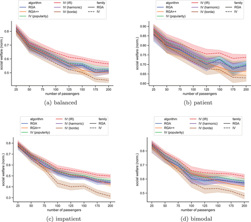
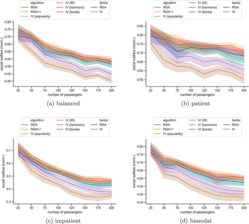
Figure 4. The social welfare, normalized by the number of passengers, in the scenario with $10$ hotspots, for each algorithm. The plots show bands of $95\mathrm{\%}$ confidence intervals.

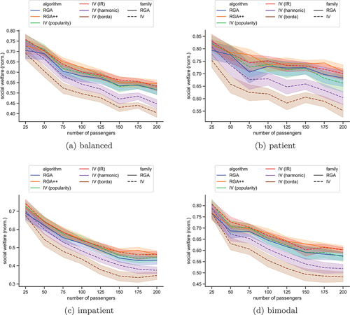
Figure 5. The social welfare, normalized by the number of passengers, in the scenario with 20 hotspots, for each algorithm. The plots show bands of $95\mathrm{\%}$ confidence intervals.

Figure 3 depicts the normalised mean social welfare of the riders when riders’ preferences over the stations are uniform. In this case, the Iterative Voting algorithm, with the instant runoff voting rule, outperforms all others. The same algorithm, with the Borda voting rule, is clearly the worst case – as we will see later, this is a recurring theme. The remaining algorithms admit quite similar performances, with IV with popularity being the second-best algorithm in most cases.

Figures 4 and 5 present the same measure when the station sampling is based on the hotspot idea, as described above. In these scenarios, Borda and harmonic rules are clearly outperformed, while all remaining rules perform quite the same. IV-IR does not yield the best social welfare, as before, although its loss compared to the best case is not large. RGA++ performs the best in most cases now. IV-Borda again performs the worst, and in this case, IV-harmonic follows at a close distance.

5.2. Fairness perspective

To measure fairness, we use the Gini Index (Gini (1912); see also, Moulin (1988)), a popular measure of wealth inequality, which is also used in the transportation literature (Yan & Howe, 2019), and has some precedence in the artificial intelligence literature (Lackner, 2020). Formally, the Gini index is defined as the following ratio:

(3) $\frac{{\sum }_{r_i\in \mathit{N}}{\sum }_{r_j\in \mathit{N}}|U_{r_i}(T_d(r_i),T_a(r_i))-U_{r_j}(T_d(r_j),T_a(r_j))|}{2{\sum }_{r_i\in \mathit{N}}{\sum }_{r_j\in \mathit{N}}{U}_{r_j}(T_d(r_j),T_a(r_j))}$(3)

where $\mathit{N}$ is the number of passenger, and $U_{r_i}$ follows Equation 1(1) $U_{r_i}(T_d,T_a)=U_{r_i}^{\mathit{d}}(T_d)+U_{r_i}^{\mathit{a}}(T_a)=\frac{{\beta }_{r_i}^{|T_d^{\ast }(r_i)-T_d(r_i)|}+{\beta }_{r_i}^{|T_a^{\ast }(r_i)-T_a(r_i)|}}{2}$(1) .

In each experiment, the Gini index is computed among the rider’s utilities, and the mean is presented in Figures 6–8. We recall that a Gini index of $0$ implies total fairness in the sense that all riders receive exactly the same utility, while an index close to $1$ implies total inequality. We also note that the Gini index should be considered in conjecture to our efficiency measures since a low Gini index implies nothing about the efficiency guarantees.⁸

Figure 6. The mean Gini index in the scenario without hotspots, for each algorithm. The plots show bands of $95\mathrm{\%}$ confidence intervals.

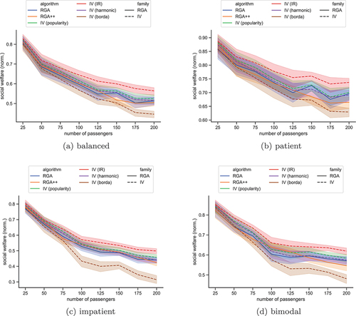
Figure 7. The mean Gini index in the scenario with $10$ hotspots, for each algorithm. The plots show bands of $95\mathrm{\%}$ confidence intervals.

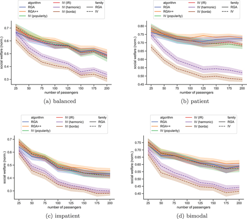
Figure 8. The mean Gini index in the scenario with 20 hotspots for each algorithm. The plots show bands of $95\mathrm{\%}$ confidence intervals.

For uniform spatial preferences (Figure 6) IV-IR returns fairer solutions. In conjecture to our efficiency results, IV-IR is clearly the best-performing algorithm from our proposals. The least fair algorithm is IR-Borda. The remaining algorithms define a middle ground with similar fairness performances.

When the spatial preferences are highly concentrated in a few hotspots, then RGA++ yields a lower Gini index in most cases. IV-Borda and IV-harmonic algorithms appear to be the least fair of all, with IV-harmonic performing slightly better between the two. In Section A in the Appendix, we employ a detailed analysis using Student’s t-test, where we compare each pair of algorithms along all possible scenarios we use.

5.3. Final remarks

As a conclusion to this section, we give some final remarks:

• IV-IR appears to be the best option in the case without hotspots, both with respect to fairness and efficiency. Our detailed analysis in Section A in the Appendix further supports this. Whenever it is not the best algorithm, it is still a reasonable choice, and it performs quite well in the cases of $10$ and $20$ hotspots, although it falls behind the RGA++ algorithm. Due to this, we believe that this algorithm is a good candidate for further investigation. A possible explanation for this success is that IV-IR, at each point, clears up TourNodes, which are undesirable by many riders. Hence, at each point, most riders need to select two choices that are not very bad for them.

• When our experiments use hotspots, the RGA++ algorithm overperforms all the other algorithms, and RGA is a reasonable choice. This is justifiable since there are only a few locations where TourNodes can be scheduled, hence the greedy approach performs well.

• In contrast, IV-Borda provides the worst results, again both with respect to fairness and efficiency, in nearly all cases. Due to these failures, this algorithm should not be considered for practical implementation.

  Rather unsurprisingly, the IV-Borda algorithm fails to perform in both measures: the rule gives a relatively high score to TourNodes, which offers very small value to some riders. For example, consider an instance where roughly half the riders prefer station $\mathit{a}$ for pick-up, half riders prefer station $\mathit{c}$, and a single rider prefers station $\mathit{b}$, and $\mathit{b}$ is closer to $\mathit{a}$ and $\mathit{b}$ than $\mathit{a}$ and $\mathit{b}$ between them, hence this is the second choice for nearly all riders: under Borda rule, location $\mathit{b}$ would be selected as the starting station, and almost all riders will not be fully satisfied. On the contrary, IV-IR, IV-popularity and IV-harmonic will never choose $\mathit{b}$. This decreases the overall sum of utilities and also increases the inequality between the riders. This phenomenon is more apparent in the cases of time-sensitive riders (see Figure 3(c)) and in the hotspot-based sampling, especially when the number of hotspots is small (see Figures 4 and 7).

• The situation is not as clear for the remaining algorithms. Most algorithms perform close to (or better than) RGA, our baseline algorithm. The RGA++ algorithm performs the best (or close to best) with respect to both objectives in highly concentrated spatial preferences. The IV-popularity algorithm is a reasonable choice, especially in the bimodal preferences example. The IV-harmonic algorithm might be useful in the uniform spatial preferences setting but suffers similarly to IV-Borda when a few stations dominate the demand. See Section A in Appendix for details.

• The RGA++ mechanism performs slightly better than RGA, both with respect to fairness and efficiency, in almost all cases explored. The same correlation is observed between IV-IR and IV-popularity.

• As the number of riders increases, the performance decreases in most cases, although some notable exceptions are observed.

• Finally, the changes in time sensitivity affect the relation between our algorithms, but not by much.

6. Related work

This work relates to three lines of research on ridesharing: (1) optimisation-oriented approaches, (2) rider satisfaction and agent-based simulations for ridesharing, and (3) game-theoretical coalition formation and voting techniques in ridesharing. Below, we go through these lines and elaborate on how the presented approach in this work relates to each.

Building on the literature on operations research, ridesharing is traditionally understood as an optimisation problem (see the extensive review of such a view in (Agatz et al., 2012)). This perspective mainly focuses on improving the service from the service providers’ point of view. For instance, the presented method in (Biswas et al., 2017) purely focuses on optimising the service with the main goal of profit maximisation, while the more recent work presented in (van der Tholen et al., 2021) looks at mixed-purpose autonomous vehicles (where goods and riders may share space in a transportation service). Then, the main focus is on the optimal use of the available space where riders and goods are both considered as preference-less entities. We deem that in such approaches, the preference of riders may be sacrificed as the course of a journey is optimised with respect to the service providers’ definition of optimality.

Another line of research (e.g., in Bistaffa et al. (2018)) is focused on providing platforms for simulating ridesharing systems and modelling their behaviour. Such approaches are crucial as they provide a test bed for evaluating different ridesharing algorithms and comparing their performance. Recently, more attention has been given to the satisfaction of riders. For instance, in Levinger et al. (2020), the authors apply data-driven techniques to learn a satisfaction function that is concerned with how riders were satisfied in previously operated ridesharing journeys. Fitting to the curve of “rider behaviour/satisfaction” would be appropriate for predictably similar domains (e.g., when the service is operating in closed settings such as ridesharing within an industrial plant). However, in more unpredictable settings (such as an urban area), bounding the current users of a service to preferences of past users may result in lower satisfaction in comparison to capturing the preferences of current users themselves.

Simulation-based analysis has been used for various topics regarding public transportation and public buses in particular. We briefly present some indicative examples in the following. Dui and Zhang (2021) simulate urban taxi sharing systems. Legêne et al. (2020) use simulations to model the impact of automated vehicles in an urban area. Wang et al. (2023) use simulation to analyse the bus bunching phenomenon, where multiple busses arrive simultaneously at the same bus stop. Sung et al. (2022) use simulations to tackle scheduling problems for electric buses. Moosavi et al. (2020) propose a simulation model to analyse and improve reliability factors, including waiting time. Multi-agent-based simulation has also been used to analyse and improve bus scheduling under different enviroments (Ap Sorratini et al., 2008; Meignan et al., 2007; Urquhart et al., 2019).

Finally, our work is related to contributions that apply game-theoretical coalition formation techniques and voting theory to ridesharing problems (Bistaffa et al., 2015; Cheng et al., 2014; Dennisen & Müller, 2016; Nourinejad & Roorda, 2016). Such approaches are related to our use of voting mechanisms but mainly focus on orthogonal problems in ridesharing or zoom on a different decision point. For instance, in (Cheng et al., 2014), the authors focus on forming rider coalitions based on the amount they are willing to pay, or in (Bistaffa et al., 2015) on how to fairly share the service cost among the riders, while our focus is mainly on how the service can operate in order to maximise rider satisfaction. Then, in both (Nourinejad & Roorda, 2016) and (Dennisen & Müller, 2016), the focus is on how the journey should start and the initiation of the journey (which complements our focus on allowing riders to participate in the route generation process). In (Nourinejad & Roorda, 2016), an agent-based model is presented for matching rider groups to vehicles using auction-based techniques. Then, cost-revenue analysis is applied to evaluate matching mechanisms based on how they ensure the (financial) survival of service providers. Finally, in (Dennisen & Müller, 2016) voting methods are used to decide riders’ coalitions to share a ride. This is orthogonal to our use of voting mechanisms to build a schedule for a ride.

7. Conclusions and future work

In this work, we presented algorithms for preference-aware dynamics ridesharing, used voting mechanisms to allow participation, and evaluated the performance as well as the utilitarian and fairness properties of the algorithms using simulation-based experiments. Such algorithms can be implemented in ridesharing services to improve the satisfaction of riders and, in turn, to foster the financial and environmental benefits of smart mobility.

Another extension to this work will be on how to nudge riders towards environmentally sustainable routes (e.g., to opt for less congested routes that may diverge from the shortest path). To that end, we envisage the applicability of incentive engineering methods (see, e.g., (Iwase et al., 2021; Protopapas et al., 2024)). Such methods necessitate integrating a bargaining phase among computational agents that represent each rider to reach a consensus on a more sustainable trajectory that is acceptable by the riders (Baarslag et al., 2017).

Data access statement

This study was a reanalysis of publicly available data from the NaPTAN dataset (Department for Transport, 2014). Implementations and data derived through the reanalysis undertaken in this study are available from the public GitHub repository at https://github.com/MaxOng99/ECS-Ridesharing.git.

Ethical statement: towards Sustainable and trustworthy smart mobility

We believe that ridesharing services are inherently sociotechnical practices. Thus, designing and developing autonomous systems for operating ridesharing should take into account both the technical and social aspects of the problem. Arguably, focusing merely on AI systems that optimise routes such that merely service providers’ benefit is maximised is an unethical practice that results in lower user satisfaction and, in turn, lower acceptability of AI-based solutions. Our work follows the idea that designing a trustworthy partnership in systems that involve humans and AI systems needs to enable dynamic interactions between the two parts and has to provide means for capturing diverse preferences of humans in the loop (Ramchurn et al., 2021).

Acknowledgments

We thank the anonymous reviewers and participants at ABMUS2022: The 6th International Workshop on Agent-Based Modelling of Urban Systems for their incisive comments that were most useful in revising this paper. The authors acknowledge the use of the IRIDIS High Performance Computing Facility and associated support services at the University of Southampton in the completion of this work. This work was supported by the UK Engineering and Physical Sciences Research Council (EPSRC) through a Turing AI Fellowship (EP/V022067/1) on Citizen-Centric AI Systems (https://ccais.ac.uk/). The authors report there are no competing interests to declare. For the purpose of open access, the authors have applied a Creative Commons Attribution (CC BY) licence to any author-accepted manuscript version arising.

Disclosure statement

No potential conflict of interest was reported by the author(s).

Supplementary material

Supplemental data for this article can be accessed online at https://doi.org/10.1080/17477778.2024.2334826

Additional information

Funding

The work was supported by the UK Engineering and Physical Sciences Research Council [EP/V022067/1].

Notes

1. A detailed discussion on how this work relates to different lines of research on ridesharing appears in Section 5.

2. The initial idea behind this work is presented at the 6th International Workshop on Agent-Based Modelling of Urban Systems (Ong et al., 2022).

3. For this, we used the publicly available Great Britain’s national dataset of public transport access points (bus stops, rail stations, airports, ferry piers, tram/metro/underground stops) (Department for Transport, 2014).

4. in the sense that not all riders have been allocated a departure and arrival time.

5. This is also known as plurality voting.

6. Also known as the Single Transferable Vote rule.

7. see, e.g., König and Grippenkoven (2020) on how the method has been implemented in the context of ridesharing.

8. Indeed, even if all utilities are negligible, then the Gini index would be $0$ if their difference would be equal.

References

- Agatz, N. A. H., Erera, A. L., Savelsbergh, M. W. P., & Wang, X. (2012). Optimization for dynamic ride-sharing: A review. European Journal of Operational Research, 223(2), 295–303. https://doi.org/10.1016/j.ejor.2012.05.028
- Aïvodji, U. M., Gambs, S., Huguet, M.-J., & Killijian, M.-O. (2016). Meeting points in ridesharing: A privacy-preserving approach. Transportation Research Part C: Emerging Technologies, 72, 239–253. https://doi.org/10.1016/j.trc.2016.09.017
- Ap Sorratini, J., Liu, R., & Sinha, S. (2008). Assessing bus transport reliability using micro-simulation. Transportation Planning and Technology, 31(3), 303–324. https://doi.org/10.1080/03081060802086512
- Baarslag, T., Kaisers, M., Gerding, E. H., Jonker, C. M., & Gratch, J. (2017). Computers that negotiate on our behalf: Major challenges for self-sufficient, self-directed, and interdependent negotiating agents. In G. Sukthankar & J. A. Rodríguez-Aguilar (Eds.), Autonomous agents and multiagent systems - AAMAS 2017 workshops, visionary papers (Vol. 10643, pp. 143–163). Springer.
- Badia, H., Argote-Cabanero, J., & Daganzo, C. F. (2017). How network structure can boost and shape the demand for bus transit. Transportation Research Part A: Policy and Practice, 103, 83–94. https://doi.org/10.1016/j.tra.2017.05.030
- Bistaffa, F., Farinelli, A., Chalkiadakis, G., & Ramchurn, S. D. (2015). Recommending fair payments for large-scale social ridesharing. In H. Werthner, M. Zanker, J. Golbeck, & G. Semeraro (Eds.), Proceedings of the 9th ACM Conference on Recommender Systems, RecSys ’15, Vienna, Austria, (pp. 139–146). ACM.
- Bistaffa, F., Rodríguez-Aguilar, J. A., Cerquides, J., & Blum, C. (2018). A simulation tool for large-scale online ridesharing. In E. André, S. Koenig, M. Dastani, & G. Sukthankar (Eds.), Proceedings of the 17th International Conference on Autonomous Agents and MultiAgent Systems, AAMAS ’18, Stockholm, Sweden, (pp. 1797–1799). ACM.
- Biswas, A., Gopalakrishnan, R., Tulabandhula, T., Mukherjee, K., Metrewar, A., & Raja-Subramaniam, T. (2017). Profit optimization in commercial ridesharing. In K. Larson, M. Winikoff, S. Das, & E. H. Durfee (Eds.), Proceedings of the 16th Conference on Autonomous Agents and MultiAgent Systems, AAMAS ’17, São Paulo, Brazil, (pp. 1481–1483). ACM.
- Boutilier, C., Caragiannis, I., Haber, S., Lu, T., Procaccia, A. D., & Sheffet, O. (2012). Optimal social choice functions: A utilitarian view. In Proceedings of the 13th ACM Conference on Electronic Commerce (EC ’12), Valencia, Spain, (pp. 197–214).
- Brandt, F., Conitzer, V., Endriss, U., Lang, J., & Procaccia, A. D. (2016). Handbook of computational social choice. Cambridge University Press.
- Cheng, S., Nguyen, D. T., & Lau, H. C. (2014). Mechanisms for arranging ride sharing and fare splitting for last-mile travel demands. In A. L. C. Bazzan, M. N. Huhns, A. Lomuscio, & P. Scerri (Eds.), International Conference on Autonomous Agents and Multi-Agent Systems, AAMAS ’14, Paris, France, (pp. 1505–1506). IFAAMAS/ACM.
- Dennisen, S. L., & Müller, J. P. (2016). Iterative committee elections for collective decision- making in a ride-sharing application. In A. L. C. Bazzan, F. Klügl, S. Ossowski, & G. Vizzari (Eds.), Proceedings of the Ninth International Workshop on Agents in Traffic and Transportation, ATT 2016, New York City, NY, USA, (Vol. 1678, pp. 1–8).
- Department for Transport. (2014). National Public Transport Access Nodes (NaPTAN). Retrieved October 5, 2021, from https://data.gov.uk/dataset/ff93ffc1-6656-47d8-9155-85ea0b8f2251/national-public-transport-access-nodes-naptan
- Dui, H., & Zhang, C. (2021). Simulations for urban taxi sharing system on routes and passengers with numerical experiments. Journal of Simulation, 15(4), 273–283. https://doi.org/10.1080/17477778.2019.1707130
- Furuhata, M., Dessouky, M., Ordóñez, F., Brunet, M.-E., Wang, X., & Koenig, S. (2013). Ridesharing: The state-of-the-art and future directions. Transportation Research Part B: Methodological, 57, 28–46. https://doi.org/10.1016/j.trb.2013.08.012
- Gini, C. W. (1912). Variabilità e mutuabilità. Contributo allo studio delle distribuzioni e delle relazioni statistiche. C. Cuppini.
- Gupta, A. K., & Nadarajah, S. (2004). Handbook of beta distribution and its applications. CRC press.
- Hasan, M. H., Van Hentenryck, P., Budak, C., Chen, J., & Chaudhry, C. (2018). Community- based trip sharing for urban commuting. Thirty-Second AAAI Conference on Artificial Intelligence AAAI-18, 32(1), 6589–6597. https://doi.org/10.1609/aaai.v32i1.12207
- Iwase, T., Stein, S., & Gerding, E. H. (2021). A polynomial-time, truthful, individually rational and budget balanced ridesharing mechanism. In Z.-H. Zhou (Ed.), Proceedings of the Thirtieth International Joint Conference on Artificial Intelligence, IJCAI-21, Montreal, Canada, (pp. 268–275). International Joint Conferences on Artificial Intelligence Organization.
- Jalali, R., Koohi-Fayegh, S., El-Khatib, K., Hoornweg, D., & Li, H. (2017). Investigating the potential of ridesharing to reduce vehicle emissions. Urban Planning, 2(2), 26–40. https://doi.org/10.17645/up.v2i2.937
- König, A., & Grippenkoven, J. (2020). Modelling travelers’ appraisal of ridepooling service characteristics with a discrete choice experiment. European Transport Research Review, 12(1), 1. https://doi.org/10.1186/s12544-019-0391-3
- Lackner, M. (2020). Perpetual voting: Fairness in long-term decision making. The Thirty- Fourth AAAI Conference on Artificial Intelligence, AAAI-20, 34(2), 2103–2110. https://doi.org/10.1609/aaai.v34i02.5584
- Legêne, M. F., Auping, W. L., Correia, G. H. D. A., & van Arem, B. (2020). Spatial impact of automated driving in urban areas. Journal of Simulation, 14(4), 295–303. https://doi.org/10.1080/17477778.2020.1806747
- Levinger, C., Hazon, N., & Azaria, A. (2020). Human satisfaction as the ultimate goal in ridesharing. Future Generation Computer Systems, 112, 176–184. https://doi.org/10.1016/j.future.2020.05.028
- Meignan, D., Simonin, O., & Koukam, A. (2007). Simulation and evaluation of urban bus- networks using a multiagent approach. Simulation Modelling Practice and Theory, 15(6), 659–671. https://doi.org/10.1016/j.simpat.2007.02.005
- Moosavi, S. M. H., Ismail, A., Yuen, C. W., & Dragan, D. (2020, May). Using simulation model as a tool for analyzing bus service reliability and implementing improvement strategies. Public Library of Science ONE, 15(5), e0232799. https://doi.org/10.1371/journal.pone.0232799
- Moulin, H. (1988). Axioms of cooperative decision making. Cambridge University Press.
- Mourad, A., Puchinger, J., & Chu, C. (2019). A survey of models and algorithms for optimizing shared mobility. Transportation Research Part B: Methodological, 123, 323–346. https://doi.org/10.1016/j.trb.2019.02.003
- Nourinejad, M., & Roorda, M. J. (2016). Agent based model for dynamic ridesharing. Transportation Research Part C: Emerging Technologies, 64, 117–132. https://doi.org/10.1016/j.trc.2015.07.016
- Ong, Y. C., Protopapas, N., Yazdanpanah, V., Gerding, H. E., & Stein, S. (2022). Preference-aware dynamic ridesharing. In M. L. Kieu, K. H. van Dam, J. Thompson, N. Malleson, A. Heppenstall, & J. Ge (Eds.), Proceedings of The 6th International Workshop on Agent- Based Modelling of Urban Systems, ABMUS 2022, Auckland, New Zealand, (p. 66–71).
- Protopapas, N., Yazdanpanah, V., Gerding, E., & Stein, S. (2024). Online decentralised mechanisms for dynamic ridesharing. In Proceedings of the 2024 International Conference on Autonomous Agents and Multiagent Systems, AAMAS ’24, Auckland, New Zealand, IFAAMAS.
- Ramchurn, S. D., Stein, S., & Jennings, N. R. (2021). Trustworthy human-AI partnerships. iScience, 24(8), 102891. https://doi.org/10.1016/j.isci.2021.102891
- Rigas, E. S., Ramchurn, S. D., & Bassiliades, N. (2014). Managing electric vehicles in the smart grid using artificial intelligence: A survey. IEEE Transactions on Intelligent Transportation Systems, 16(4), 1619–1635. https://doi.org/10.1109/TITS.2014.2376873
- Robusto, C. C. (1957). The cosine-haversine formula. The American Mathematical Monthly, 64(1), 38–40. https://doi.org/10.2307/2309088
- Stein, S., & Yazdanpanah, V. (2023). Citizen-centric multiagent systems. In N. Agmon, A. An, A. Ricci, & W. Yeoh (Eds.), Proceedings of the 2023 International Conference on Autonomous Agents and Multiagent Systems, AAMAS ’23, London, United Kingdom, (pp. 1802–1807). ACM.
- Sung, Y.-W., Chu, J. C., Chang, Y.-J., Yeh, J.-C., & Chou, Y.-H. (2022). Optimizing mix of heterogeneous buses and chargers in electric bus scheduling problems. Simulation Modelling Practice and Theory, 119, 102584. https://doi.org/10.1016/j.simpat.2022.102584
- Transport for London. (2021). Buses Performance Data. Retrieved October 8, 2021, from https://tfl.gov.uk/corporate/publications-and-reports/buses-performance-data
- Urquhart, N., Powers, S., Wall, Z., Fonzone, A., Ge, J., & Polhill, J. G. (2019). Simulating the actions of commuters using a multi-agent system. Journal of Artificial Societies and Social Simulation, 22(2), 10. https://doi.org/10.18564/jasss.4007
- van der Tholen, M., Beirigo, B. A., Jovanova, J., & Schulte, F. (2021). The share-a-ride problem with integrated routing and design decisions: The case of mixed-purpose shared autonomous vehicles. In M. Mes, E. Lalla-Ruiz, & S. Voß (Eds.), Computational logistics (pp. 347–361). Springer International Publishing.
- Wang, X., Liu, T., & Xu, M. (2023). Bus bunching simulation based on the lattice Boltzmann model of traffic flow. SIMULATION, 99(2), 183–199. https://doi.org/10.1177/00375497221112915
- Yan, A., & Howe, B. (2019). Fairness in practice: A survey on equity in urban mobility. Quarterly Bulletin of the Computer Society if the IEEE Technical Committee, 42(3), 49–63.
- Zavvos, E., Gerding, E. H., Yazdanpanah, V., Maple, C., Stein, S., & Schraefel, M. C. (2022). Privacy and trust in the internet of vehicles. IEEE Transactions on Intelligent Transportation Systems, 23(8), 10126–10141. https://doi.org/10.1109/TITS.2021.3121125
- Zhang, R., Spieser, K., Frazzoli, E., & Pavone, M. (2015). Models, algorithms, and evaluation for autonomous mobility-on-demand systems. In American Control Conference, ACC 2015, Chicago, IL, USA, (pp. 2573–2587). IEEE.