The magnetic method as a tool to investigate the Werenskioldbreen environment (south-west Spitsbergen, Arctic Norway)

ABSTRACT

We used a novel approach of applying magnetic analyses to investigate the material released from the receding glacier Werenskioldbreen on Spitsbergen, Svalbard, Arctic Norway. Surface sediments were taken from the bay Nottinghambukta and the Werenskioldbreen foreland, along two main proglacial streams. Magnetic analyses, namely the low-field mass magnetic susceptibility, anhysteretic susceptibility mass normalized and hysteresis parameters, served to determine magnetic properties and identify the magnetic composition of the study material. We selected two distinct types of sediments. The first group, consisting of magnetite and pyrrhotite, has more single-domain grains in comparison to the second one, containing only magnetite. In the second group, multi-domain particles dominate. Deposits from the north stream, glacier river and an area close to the estuary of Nottinghambukta include magnetite and pyrrhotite. Magnetite was found in the south stream and in the outside part of the bay. Magnetic composition reflects different source rocks of sediments. This study demonstrates the utility of the magnetic method in analysing the current state of glacier environments.

KEYWORDS:

• Environmental magnetism
• glacier environment
• surface sediments
• Svalbard
• magnetic susceptibility

ABBREVIATIONS:

• κ(T): low-field volume magnetic susceptibility dependence on temperature
• MD: multi-domain particles
• SD: single-domain particles
• χ_ARM: mass-normalized anhysteretic susceptibility
• χ_LF: low-field mass magnetic susceptibility

Introduction

Global climate change has a significant effect on polar regions. The Arctic environment is rapidly changing. Annual and seasonal temperatures have been rising in the Arctic, and sea-ice volume and extent have been declining (Solomon et al. 2007; Kwok et al. 2009). To understand such changes, there is a need to investigate natural archives, such as marine sediments, soil and ice cores, especially in polar regions, where the magnitude of expected changes is the most distinct and rapid (e.g.,Holland & Bitz 2003; Miller et al. 2010; Stocker et al. 2013; Thienpont et al. 2015). Glacier melting is one of the environment’s responses to global climate change; therefore, it is very important to understand this process and its extent through the application of standard and non-standard methods.

Environmental magnetism is a multidisciplinary subject that connects research on a wide range of topics (e.g., Evans & Heller 2003). All materials respond to an applied magnetic field. Iron-bearing minerals are sensitive to environmental processes, which makes magnetic techniques highly useful for detecting signals associated with natural processes. In environmental magnetism, rock and mineral magnetic methods are used to study the formation, transportation, deposition and postdepositional modifications of magnetic minerals under the impacts of a wide range of natural processes (e.g., Liu et al. 2012). Reports documenting the application of the magnetic methods to investigate glacial environment are mainly focused on climatic changes in sedimentary sequences (e.g., Lanci et al. 1999; Sagnotti et al. 2001; Hirt et al. 2003; Hatfield et al. 2016) or ice sequences (e.g., Lanci et al. 2001; Lanci & Delmonte 2013). This paper presents the application of magnetic analyses to the study of the current state of glacier environment. This novel approach can provide new information in the area of glacier study.

Study area

The glacier Werenskioldbreen is located in the south-western part of Wedel Jarlsberg Land on Spitsbergen, Svalbard, Arctic Norway (Fig. 1). The glacier is 9.5 km long (Hagen & Lefauconnier 1995) and covers 44.1 km², of which 61% are glaciated (Ignatiuk et al. 2014). The Werenskioldbreen catchment area includes two main proglacial streams, separated by a medial moraine, and is closed by an ice-cored frontal moraine from the west (Majchrowska et al. 2015). The thickness of Werenskioldbreen is around 100–140 m, with a surface layer of cold ice (50 –100 m) and temperate ice below (Pälli et al. 2003). This polythermal glacier, terminating on land, has been in a state of constant recession since the 1920s (Kosiba 1960).

Figure 1. Lithostratigraphy of the Werenskioldbreen basin, modified after Stachnik et al. (2016). All subdivided units belong to the Heckla Hoek Succession.

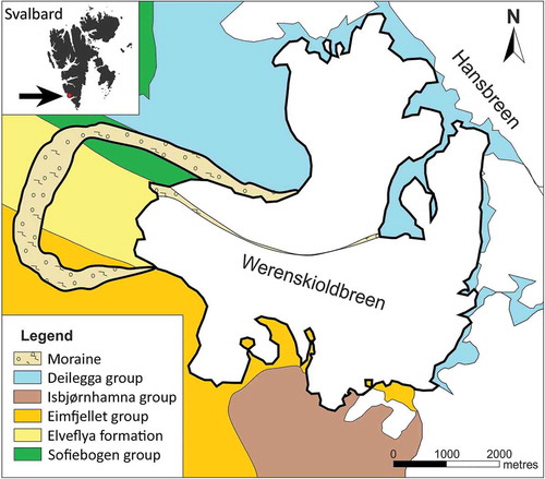
Geologically, Werenskioldbreen is located in the contact zone of three tectonic blocks of the Hecla Hoek Succession (Fig. 1; Czerny et al. 1993). The Hecla Hoek Succession is a collection of rocks older than Devonian, and involved in Caledonian orogenic deformation in Svalbard (Birkenmajer 1990). The Eimfjellet group underlies the southern and south-western part of the glacier and includes amphibolite, quartzite and chlorite schist. The Deilegga group, belonging to the north tectonic block, forms the eastern and northern part of the Werenskioldbreen basin. It is mainly composed of phyllites with quartzite and silt intercalations, and calcareous and chlorite schists (Kieres & Piestrzynski 1992). The Sofiebogen group, consisting of green schists, and muscovite–carbonate–quartz or carbonate–chlorite–quartz schists, is located in the north-western part of the basin. The Sofiebogen group includes the Elveflya formation, which consists of similar rocks. The proglacial area belongs to the Sofiebogen and Eimfjellet groups, where mica–carbonate–quartz and grey calcite marbles dominate (Czerny et al. 1993). The Isbjørnhamna group contains garne–mica schists intercalated with grey marbles alternating with schists, and underlies the area to the south of Werenskioldbreen (Birkenmajer 1990).

The bay Nottinghambukta is a very shallow embayment of the Greenland Sea (only 2.5 m below the lowest tide). The exposed surface can be more than 50% of the bay (Giżejewski 1986). A delta, supplied by the proglacial streams of Werenskioldbreen, progrades into the bay from the east. From the west, it is partially screened from the open sea by the Dunøyane islands. Nottinghambukta is a very young form, having been created by depositional activity of proglacial rivers and, at the same time, essentially influenced by marine processes, such as tides, waves and coastal currents (Kowalska & Sroka 2008).

The research area is lithologically differentiated by the occurrence of different minerals with various magnetic properties (e.g., pyrrhotite, magnetite and hematite). Magnetic properties of sediments are directly associated with the origin of detrital material and can vary depending on the mineralogy of the source rock, especially iron compounds, which makes it possible to determine the source of sediments.

The primary aim of this paper is to provide a description of mineral material released from ice masses during the recession of Werenskioldbreen, through the evaluation of their magnetic signature.

Methods

Sampling

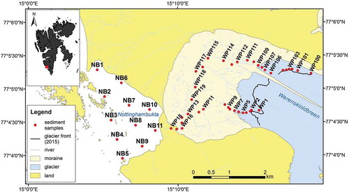
A total of 49 surface sediment samples were taken from the seafloor of Nottinghambukta, along the two main proglacial streams, located in the north and in the south, and from the Werenskioldbreen proglacial river formed by these streams (Table 1, Fig. 2). The streams are separated by a medial moraine and transport what is likely to be different material from the opposite sides of Werenskioldbreen. Specimens were taken close to watercourses, where material had recently been uncovered. Marine sediment collection was performed from a pontoon equipped with the Van Veen grab sampler, from a depth of about 1–3 m. A sample of 1 kg was gathered from each sampling point. Specimens were collected in 2015, transported to a laboratory and stored at −20°C. Before measurements, sediment samples were dried to constant weight.

Table 1. Grouping of investigated samples into sets.

Set of samples	Sample
Nottinghambukta	NB1-11
North stream	WP100-119
South stream	WP1-11
Glacier river	WP12-18

Figure 2. Location map of analysed samples (based on Norwegian Polar Institute maps at http://toposvalbard.npolar.no/). The glacier front was drawn based on the Landsat 8 satellite image from 8 September 2015 (available from the US Geological Survey at https://earthexplorer.usgs.gov/).

Characterization of study material

Studied material was characterized by means of grain-size determination. The analysis of grain size distribution was performed in the Laboratory of Applied Geology of the Institute of Oceanography, University of Gdańsk. Grain size distribution was determined by dry sieving with nylon sieves. This analysis determines the particle size > 0.063 mm. Results of sieve analysis were entered into Gradistat programme (Blott & Pye 2001). Using this programme, we calculated the mean grain size according to the formulas of Folk & Ward (1957). Six types of grain size were separated based on the mean: coarse sand (> 500 µm), medium sand (250–500 µm), fine sand (125–250 µm), very fine sand (63–125 µm), very coarse silt (31–63 µm) and coarse silt (16–31 µm). The last two grain sizes were estimated only theoretically, by calculation.

Preliminary grain size distribution results showed that fine sand occurs close to the estuary in Nottinghambukta (NB9-11). Further away from the estuary (NB1-8), very fine sand and very coarse silt prevail. In the north stream, the main grain size is between coarse silt and medium sand, with very fine sand predominating. Fine and very fine sand dominates in the south stream, with the exception of two samples (medium sand in sample WP1 and coarse sand in WP2), while the glacier river is additionally enriched with a finer fraction (very coarse and coarse silt).

Magnetic methods

Measurements of χ_LF were conducted using the MFK1-FA multi-function Kappabridge instrument (Agico, Czech Republic). Anhysteretic remanence magnetization was measured by means of 2G SQUID cryogenic magnetometer. To acquire anhysteretic remanence magnetization, each sample was exposed to an alternating current magnetic field with peak field amplitude decreasing from 100 to 0 mT and a superimposed direct current bias field of 100 μT. χ_ARM was obtained by dividing the anhysteretic remanence magnetization by the value of the direct current bias field. The χ_ARM parameter served to determine the role of single-domain magnetite for material with one magnetic phase (e.g., magnetite). Both χ_LF and χ_ARM depend also on the concentration of magnetic minerals. Identification of magnetic minerals was based on a thermomagnetic experiment: low-field volume magnetic susceptibility dependence on temperature – κ(T). The evolution of κ(T) experiments was measured using a Kappabridge KLY-3 with high-temperature extension CS-3 (Agico). The experiment was conducted in the air during heating in the 20–700°C temperature range and cooling to 20°C. Hysteresis loop measurements were performed at room temperature, using the Vibrating Sample Magnetometer, produced by Molspin (UK), and vibrational magnetometer Micro-Mag AGFM 2900–02 (USA). Sediment samples used for this experiment weighted 0.3 g and 0.006 g, respectively. Both devices operated at the maximum magnetic field of 1 T. The hysteresis loops allowed for the determination of the coercivity (H_c), saturation remanence (M_rs) and saturation magnetization (M_s). The coercivity of remanence (H_cr) was determined using the curves of subsequent direct current back-field remagnetization of M_rs. Based on these parameters, a Day-Dunlop diagram (Day et al. 1977; Dunlop 2002a, b) was created. The domain state of magnetic grains was inferred from the position of data on the diagram in relation to the corresponding mixing lines.

Magnetic analyses were performed in the Paleomagnetic Laboratory of the Institute of Geophysics, Polish Academy of Sciences, in Warsaw.

Results and discussion

Magnetic analyses

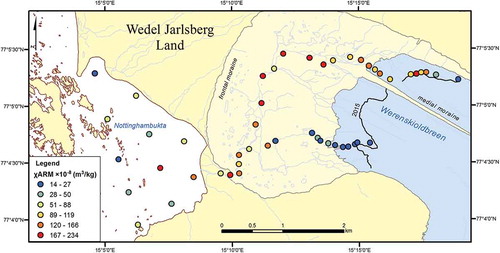
Low-field susceptibility and anhysteretic susceptibility values varied considerably from sample to sample (Figs. 3, 4). Generally, χ_LF values were between 20 and 30 × 10⁻⁸m³/kg. However, the highest χ_LF value for Nottinghambukta (70.81 × 10⁻⁸m³/kg) was obtained for the sample from the southernmost point of the bay (NB5), where boat launching occurred for many years. Pollution by motor oil and other contamination of anthropogenic origin affect χ_LF, usually increasing its value. Only in the middle part of the north stream, high values of 60.64–75.30 × 10⁻⁸m³/kg were detected. χ_ARM values were in the range of 25.47–77.95 × 10⁻⁸m³/kg for Nottinghambukta sediments, except for two specimens (NB8, NB11), which had higher values (χ_ARM> 143 × 10⁻⁸m³/kg). Samples from the north stream achieved the highest χ_ARM values (87 <χ_ARM< 234 × 10⁻⁸m³/kg), except for the first two specimens, for which χ_ARM was about 23–33 × 10⁻⁸m³/kg. By contrast, the south stream was characterized by a rather low χ_ARM values (13.98 – 40.76 × 10⁻⁸m³/kg), up to the area where both streams combine and create a glacier river. Along the glacier river, χ_ARM exceeded 79 × 10⁻⁸m³/kg. The variability seen in χ_LF and χ_ARM results from the different bedrocks eroding along the north and the south streams. The geological unit along the latter – the Elveflya formation – consists mainly of metamorphosed volcaniclastic rocks, while that along the north stream – the Deilegga group – mainly comprises metamorphosed sedimentary rocks (Fig. 1).

Figure 3. Distribution of χ_LF in the investigated area (based on Norwegian Polar Institute maps at http://toposvalbard.npolar.no/).

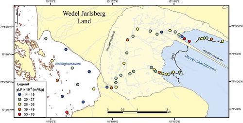
Figure 4. Distribution of χ_ARM in the investigated area (based on Norwegian Polar Institute maps at http://toposvalbard.npolar.no/).

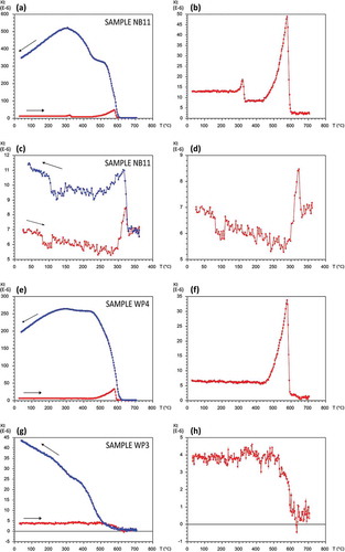
Selected representative examples of the thermomagnetic curves are given in Fig. 5. In Fig. 5a and b, the heating curves have two peaks in temperatures just below 320°C and 590°C, the distinguishing Curie temperatures for pyrrhotite and magnetite, respectively. The first peak below 320°C can be partly due to the Hopkinson effect (Hopkinson 1890) and partly to creating a new magnetic mineral. The pyrrhotite Hopkinson peak is clearly visible on the cooling curve of partial κ(T) analysis (Fig. 5c).The second peak probably results from magnetite formation due to heating. The heating curves also illustrate a plateau of susceptibility between 330°C and 440°C that can be interpreted as the occurrence of initial magnetite (Fig. 5b). The newly formed magnetite dominates the initial magnetic mineralogy during cooling (Fig. 5a). The decrease of κ on the cooling curve between 300°C and room temperature can be attributed to the progressing transformation of the newly formed magnetite. Similar κ(T) curves were reported by Crouzet et al. (2001) in Himalayan metacarbonates and characterized as a Hopkinson peak of pyrrhotite. These are typical curves for most Nottinghambukta specimens, characteristic also of sediments from the north stream and the glacier river. Heating curves of κ(T) for samples from the south stream and a few samples from the bay (NB1, NB3, NB5) are impeded by thermochemical changes above 400°C, which trigger the formation of new magnetite (Fig. 5e). Several κ(T) heating curves are relatively constant, until the temperature reaches 580–590°C, the Curie point of magnetite, where susceptibility decreases to zero (Fig. 5g, h; Dunlop & Özdemir 1997). The cooling curve shows the creation of magnetite at a temperature higher than 590°C. Furthermore, all presented curves show a rather constant susceptibility in the low temperature range (up to 250°C) indicating a minor contribution of paramagnetic minerals to the bulk low-field susceptibility. To sum up, the sediments can be divided into two groups in terms of magnetic mineralogy: samples containing only magnetite and those with both magnetite and pyrrhotite.

Figure 5. κ(T) conducted in the air with heating curves (red) and cooling curves (blue). (a, b) Typical diagrams for most samples of Nottinghambukta, characteristic also of the north stream and the glacier river. (c, d) Partial κ(T) analysis for the NB11 sample. (e, f) Typical diagrams for the south stream, characteristic also of the outside part of the bay. (g, h) Examples of untypical diagrams from the south stream. In the graphs in the right column (b, d, f, h) the heating curves are shown with enlarged scales on the y axes, providing more detail.

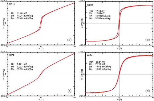
Figure 6 shows examples of hysteresis loops for the samples with (Fig. 6a, b) and without (Fig. 6c, d) pyrrhotite. Specimens with pyrrhotite exhibit a slightly wasp-waisted shape (Fig. 6b). Samples without pyrrhotite (with only magnetite) show a greater contribution of paramagnetic minerals (Fig. 6c) than those with magnetite and pyrrhotite (Fig. 6a). However, loops for both groups of specimens exhibit a ferrimagnetic behaviour.

Figure 6. Example of hysteresis loops for a sample (a, b) with and (c, d) without pyrrhotite. The graphs on the right (b, d) display loops after paramagnetic correction.

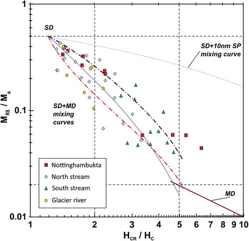
Hysteresis parameters, present on the Day-Dunlop graph, indicate the grain size of magnetic fraction. Sediments under analysis are mainly a mixture of SD and MD particles (Fig. 7). However, samples occur mostly in the upper left part of the graph, where SD grains dominate. Specimens from the outside part of Nottinghambukta (NB1-3, NB5) and those from close to the front of Werenskioldbreen (WP1-2, WP4-9, WP100-101, WP106, WP111) have a greater content of MD particles. This division may be caused by the presence of pyrrhotite in samples from the upper left part of plot. The critical SD grain size for equidimensional pyrrhotite is 1.6 µm (Dunlop & Özdemir 1997). Based on data from Clark (1984), the values of magnetization and coercivity ratios for SD pyrrhotite are 0.407–0.474 and 1.35, respectively. Peters & Dekkers (2003) observed that this mineral affects the position of samples on a Day-Dunlop diagram by shifting it towards SD grains.

Figure 7. Day-Dunlop graph showing the hysteresis magnetization ratio (M_rs/M_s) versus coercivity ratio (H_cr/H_c) (Day et al. 1977; Dunlop 2002a, b). Dotted line represents theoretically calculated mixing curve of single-domain with superparamagnetic grains (SD + 10 nm SP). Dashed curves represent different mixing curves of single–domain and multi–domain particles (SD + MD).

The other indicators of magnetic grain size distribution and mineralogy are χ_ARM versus χ_LF and χ_ARM versus M_rs relations (Fig. 8). The plot of χ_ARM versus χ_LF shows two linear trends (Fig. 8a). A linear trend indicates a generally constant distribution of grain size and mineralogy (King et al. 1982). The two trends represent two groups of samples which differ in mineralogy and grain-size distribution. Division between the studied sets of samples is clearly visible. Most of the Nottinghambukta sediments occur in the initial part of the first trend. The samples from the north stream and the glacier river are presented in the upper part of this trend, where two specimens from the bay (NB8 and NB11) are also placed. Samples from the south stream and a few specimens from the north stream and the Nottinghambukta (WP1-11, WP100-101, WP106-107, NB1-3, NB5) are the basis of the second trend. The group of samples from the first trend is characterized by the 3.25–9.5 range of χ_ARM/χ_LF values, while specimens from the second trend have this ratio mainly between 0.55 and 2.13. According to Peters & Dekkers (2003), these are the typical ranges for SD and MD grains, respectively, assuming that the mixture of magnetite and pyrrhotite demonstrates similar properties of χ_ARM/χ_LF as homogeneous magnetite. It means that pyrrhotite influences χ_ARM value in a similar way as SD magnetite.

Figure 8. Plots of (a) χ_ARM versus χ_LF (King et al. 1982) and (b) anhysteretic magnetic susceptibility versus saturation magnetization (M_rs).

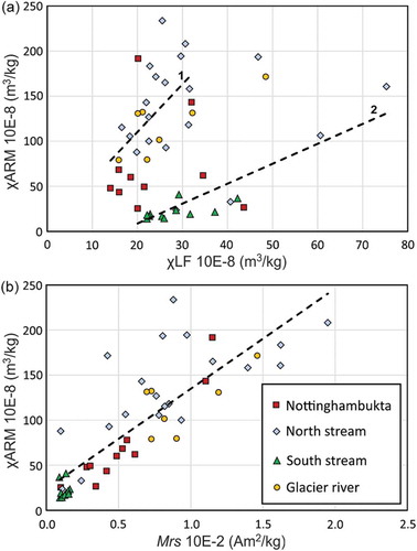
The χ_ARM versus M_rs graph demonstrates concentration of SD grains in relation to the total grain size (Fig. 8b). The relation between χ_ARM and M_rs forms one linear trend. Particular groups of samples occupy different parts of the diagram. Specimens NB1, WP100, WP101 and those from the south stream are clustered at the very beginning of the graph. Next, there is the Nottinghambukta set of samples, except for two specimens (NB8 and NB11), which are in the last group, with sediments from the glacier river and several samples from the north stream. These groups form a linear trend. Samples plotted along this trend differ mainly in concentration. The north stream set of samples is slightly shifted from the line to higher χ_ARM values, indicating higher content of SD grains.

Comparing both plots (Fig. 8), we observe two grain-size trends in χ_ARM versus χ_LF and only one in χ_ARM versus M_rs. It could be the influence of paramagnetic minerals which contribute to low-field susceptibility but not to saturation remanence. Additionally, we see that most sediments from the north stream are clustered in one group, while those from the south stream form a second group. The samples from Nottinghambukta and the glacier river are spread in between. The first group contains material with heterogeneous magnetic properties, whereas the second group exhibits similar and more homogeneous magnetic properties. The geological setting of the studied area suggests that this is probably the result of different parent rocks. Along the south stream, the parent rock is of volcaniclastic origin. In contrast, material transported by the north stream mainly are delivered from metamorphosed sedimentary rocks, which results in a more heterogeneous composition and magnetic properties. Sediments from the glacier river have a mixture of both and flow into Nottinghambukta. The farther from the estuary, the more homogeneous the sediments.

Conclusions

This study demonstrates the novel approach of applying the magnetic method to the analysis of a glacier environment. The magnetic method enables us to distinguish two sets of deposited materials which differ by magnetic mineralogy. The first set consists of a mixture of pyrrhotite and magnetite with predominantly finer grains of SD structure. The second set contains magnetite with larger grains of MD structure. This division allows us to ascribe different parent rock to each set: metamorphosed sedimentary rocks from the northern edge of the glacier to the first set and metamorphosed volcaniclastic rocks from the southern edge to the second set.

Heterogeneous χ_LF distribution along both streams, the river and the bay, independent of the magnetic composition, suggests that various χ_LF values could be caused by changes in concentrations of magnetic minerals due to some inhomogeneity of the parent rock, including another – unknown – source of the investigated material. On the other hand, variations in the speed of glacier melting might be responsible for differentiated sorting of the material. The presented study poses new questions to be addressed in the future.

Acknowledgements

The authors would like to thank Tomasz Gonet for assistance in the collection of samples. The authors are grateful to Pedro Silva, Simo Spassov and an anonymous reviewer for their helpful comments and suggestions to the manuscript.

Disclosure statement

No potential conflict of interest was reported by the authors.

Additional information

Funding

This work was partially financed by funds from the Leading National Research Centre, received by the Centre for Polar Studies for the period 2014-18, and also supported by the Polish Ministry of Science and Higher Education under statutory activities no. 3841/E-41/S/2015.

References

- Birkenmajer K. 1990. Geology of the Hornsund area, Spitsbergen. Geological map 1:75000, with explanations. Katowice: Polish Academy of Sciences, Committee on Polar Research, and Silesian University.
- Blott S.J. & Pye K. 2001. Gradistat: a grain size distribution and statistics package for the analysis of unconsolidated sediments. Earth Surface Processes and Landforms 26, 1237–9.
- Clark D.A. 1984. Hysteresis properties of size dispersed monoclinic pyrrhotite grains. Geophysical Research Letters 11, 173-176.
- Crouzet C., Stang H., Appel E., Schill E. & Gautam P. 2001. Detailed analysis of successive pTRMs carried by pyrrhotite in Himalayan metacarbonates: an example from Hidden Valley, Central Nepal. Geophysical Journal International 146, 607–618.
- Czerny J., Kieres A., Manecki M. & Rajchel J. 1993. Geological map of SW part of Wedel Jarlsberg Land, Spitsbergen 1:25 000. Kraków: Institute of Geology and Mineral Deposits.
- Day R., Fuller M. & Schmidt V.A. 1977. Hysteresis properties of titanomagnetites: grain-size and compositional dependence. Physics of the Earth and Planetary Interiors 13, 260–267.
- Dunlop D.J. 2002a. Theory and application of the Day plot (Mrs/Ms versus Hcr/Hc) 1. Theoretical curves and tests using titanomagnetite data. Journal of Geophysical Research—Solid Earth 107, article no. 2056, doi: 10.1029/2001JB000486.
- Dunlop D.J. 2002b. Theory and application of the Day plot (Mrs/Ms versus Hcr/Hc) 2. Application to data for rocks, sediments, and soils. Journal of Geophysical Research—Solid Earth 107, article no. 2057, doi: 10.1029/2001JB000487.
- Dunlop D.J. & Özdemir Ö. 1997. Rock magnetism: fundamentals and frontiers. Cambridge: Cambridge University Press.
- Evans M.E. & Heller F. 2003. Environmental magnetism: principles and applications of enviromagnetics. San Diego: Academic Press.
- Folk R.L. & Ward W.C. 1957. Brazos River bar: a study in the significance of grain-size parameters. Journal of Sedimentary Petrology 27, 3–26.
- Giżejewski J. 1986. Inter- and subtidal sedimentation in the Nottingham Bay, South Spitsbergen. Acta Geologica Polonica 36, 347–355.
- Hagen J.O. & Lefauconnier B. 1995. Reconstructed runoff from the High Arctic basin Bayelva based on mass-balance measurements. Nordic Hydrology 26, 285–296.
- Hatfield R.G., Reyes A.V., Stoner J.S., Carlson A.E., Beard B.L., Winsor K. & Welke B. 2016. Interglacial responses of the southern Greenland ice sheet over the last 430,000 years determined using particle-size specific magnetic and isotopic tracers. Earth and Planetary Science Letters 454, 225–236.
- Hirt A.M., Lanci L. & Koinig K. 2003. Mineral magnetic record of Holocene environmental changes in Sägistalsee, Switzerland. Journal of Paleolimnology 30, 321–331.
- Holland M.M. & Bitz C.M. 2003. Polar amplification of climate change in coupled models. Climate Dynamics 21, 221–232.
- Hopkinson J. 1890. Magnetic properties of alloys of nickel and iron. Proceedings of the Royal Society of London 48, 292–295.
- Ignatiuk D., Piechota A.M., Ciepły M. & Luks B. 2014. Changes of altitudinal zones of Werenskioldbreen and Hansbreen in period 1990-2008, Svalbard. AIP Conference Proceedings 1618, 275–280.
- Kieres A. & Piestrzynski A. 1992. Ore-mineralization of the Hecla Hoek Succession (Precambrian) around Werenskioldbreen, south Spitsbergen. Studia Geologica Polonica 98, 115–151.
- King J.W., Banerjee S.K., Marvin J.A. & Özdemir Ö. 1982. A comparison of different magnetic methods for determining the relative grain size of magnetite in natural materials: some results from lake sediments. Earth and Planetary Science Letters 59, 404–419.
- Kosiba A. 1960. Some results of glaciological investigations in SW-Spitsbergen carried out during the Polish I.G.Y. Spitsbergen Expedition in 1957, 1958 and 1959. Zeszyty Naukowe Uniwersytetu Wrocławskiego B4. Wrocław: University of Wrocław.
- Kowalska A. & Sroka W. 2008. Sedimentary environment of the Nottinghambukta delta, SW Spitsbergen. Polish Polar Research 29, 245–259.
- Kwok R., Cunningham G.F., Wensnahan M., Rigor I., Zwally H.J. & Yi D. 2009. Thinning and volume loss of the Arctic Ocean sea ice cover: 2003-2008. Journal of Geophysical Research—Oceans 114, C07005, doi: 10.1029/2009JC005312.
- Lanci L. & Delmonte B. 2013. Magnetic properties of aerosol dust in peripheral and inner Antarctic ice cores as a proxy for dust provenance. Global and Planetary Change 110, 414–419.
- Lanci L., Hirt A.M., Lowrie W., Lotter A.F., Lemke G. & Sturm M. 1999. Mineral magnetic record of late Quaternary climatic changes in a high alpine Lake. Earth and Planetary Science Letters 170, 49–59.
- Lanci L., Kent D.V., Biscaye P.E. & Bory A. 2001. Isothermal remanent magnetization of Greenland ice: preliminary results. Geophysical Research Letters 28, 1639–1642.
- Liu Q., Roberts A.P., Larrasoana J.C., Banerjee S.K., Guyodo Y., Tauxe L. & Oldfield F. 2012. Environmental magnetism: principles and applications. Reviews of Geophysics 50, RG4002, doi: 10.1029/2012RG000393.
- Majchrowska E., Ignatiuk D., Jania J., Marszałek H. & Wąsik M. 2015. Seasonal and interannual variability in runoff from the Werenskioldbreen catchment, Spitsbergen. Polish Polar Research 36, 197–224.
- Miller G.H., Alley R.B., Brigham-Grette J., Fitzpatrick J.J., Polyak L., Serreze M.C. & White J.W.C. 2010. Arctic amplification: can the past predict the future?Quaternary Science Reviews 29, 1679–1715.
- Pälli A., Moore J.C., Jania J., Kolondra L. & Glowacki P. 2003. The drainage pattern of Hansbreen and Werenskioldbreen, two polythermal glaciers in Svalbard. Polar Research 22, 355–371.
- Peters C. & Dekkers M.J. 2003. Selected room temperature magnetic parameters as a function of mineralogy, concentration and grain size. Physics and Chemistry of the Earth 28, 659–667.
- Sagnotti L., Macri P., Camerlenghi A. & Rebesco M. 2001. Environmental magnetism of Antarctic Late Pleistocene sediments and interhemispheric correlation of climatic events. Earth and Planetary Science Letters 192, 65–80.
- Solomon S., Qin D., Manning M., Chen Z., Marquis M., Averyt K.B., Tignor M. & Miller H.L. (eds.) 2007. Contribution of Working Group I to the fourth assessment report of the Intergovernmental Panel on Climate Change. Cambridge: Cambridge University Press.
- Stachnik Ł., Majchrowska E., Yde J.C., Nawrot A., Cichała–Kamrowska K., Ignatiuk D. & Piechota A. 2016. Chemical denudation and the role of sulfide oxidation at Werenskioldbreen, Svalbard. Journal of Hydrology 538, 177–193.
- Stocker T.F., Qin D., Plattner G.K., Tignor M., Allen S.K., Boschung J., Nauels A., Xia Y., Bex V. & Midgley P.M. (eds.) 2013. Climate change 2013. The physical science basis. Contribution of Working Group I to the fifth assessment report of the Intergovernmental Panel on Climate Change. Cambridge: Cambridge University Press.
- Thienpont J.R., Korosi J.B., Cheng E.S., Deasley K., Pisaric M.F.J. & Smol J.P. 2015. Recent climate warming favours more specialized cladoceran taxa in western Canadian Arctic lakes. Journal of Biogeography 42, 1553–1565.