A spatiotemporal comprehensive constraint interpolation method for missing values in monthly composite Suomi-NPP VIIRS Cloud Mask images

ABSTRACT

The Earth’s nighttime light imaging data collected by the Visible Infrared Imaging Radiometer Suite Day/Night Band (VIIRS DNB) are severely lost in summer, hindering the further application of VIIRS DNB data. In this article, a spatiotemporal comprehensive constraint interpolation method (SCIM) that accounts for the relative stationarity of temporal nighttime light, spatial correlations and heterogeneity among pixels is designed. Meanwhile, the method considers the seasonal fluctuations in nighttime light radiation, introduces spatial autocorrelation coefficients and spatial heterogeneity coefficients, and solves the problem of missing VIIRS DNB data. First, 8 widely used temporal interpolation methods (TIM) are selected to perform temporal interpolation for missing image data. Second, the existing VIIRS monthly images are used to construct the constraint relationship between time and space, and the pixels that do not meet the constraint conditions in the TIM simulation image are removed. The inverse distance weight (IDW) method is applied to the removed null pixels to obtain the image simulated by the SCIM. Finally, the accuracy of the TIM and SCIM is evaluated. The results show that the accuracy of the SCIM-simulated image is better than that of the TIM-simulated image. The proposed approach improves the quality of the VIIRS DNB dataset.

KEYWORDS:

• VIIRS Cloud Mask
• temporal interpolation methods
• spatiotemporal comprehensive constraint interpolation
• spatial autocorrelation
• inverse distance weight

Highlights

1. Spatiotemporal comprehensive constraint interpolation method for VIIRS vcm image interpolation.

2. A method that accounts for the relative stationarity of temporal nighttime light, spatial correlation and heterogeneity between pixels.

3. Considering the influence of seasonal fluctuation of nighttime light radiation and the stability of urban spatial structure.

4. The spatial autocorrelation coefficient and spatial heterogeneity coefficient are introduced.

5. Comparative analysis of time series interpolation method and spatiotemporal comprehensive constraint interpolation method.

1. Introduction

Nighttime light remote sensing, as an important and active branch of remote sensing application research and development, has received increasing attention in recent years (Chen et al. 2019; Elvidge et al. 2017; 2021, 2022; Li and Li 2015). Unlike traditional optical remote sensing satellites that obtain ground radiation information, nighttime light remote sensing is the acquisition of visible near-infrared electromagnetic wave information emitted from the surface under cloudless conditions at night (Levin et al. 2020). Compared to that in ordinary remote sensing satellite images, the surface light intensity information recorded by nighttime light images can more directly reflect the intensity differences of human activities in different regions (Ma et al. 2014; Zheng et al. 2023) and is therefore widely used in analyses of urbanization processes (Fan et al. 2014; 2019; Imhoff et al. 1997; Ma et al. 2012; Sun et al. 2021), artificial impermeable surface extraction (Guo et al. 2015), the spatial estimation of socioeconomic indicators (Elvidge et al. 2009; Man, Hirakawa, and Hiromichi 2021; Ustaoglu, Bovkır, and Aydınoglu 2021), major event assessment (Elvidge et al. 2020; Tveit, Skoufias, and Strobl 2022), ecological environment assessment (Gaston et al. 2013; Jiang et al. 2022), and other fields.

Nighttime light data obtained from satellite observations has become one of the most widely used geospatial data products in the scientific community. Initially, the Operational Linescan System (OLS) of the US Air Force Defense Meteorological Satellite Program (DMSP) collected low-level imaging data from 1992 to 2013, and the data were compiled into the annual nighttime lighting dataset by the National Geophysical Data Center (NGDC) of the National Oceanic and Atmospheric Administration (NOAA). However, the DMSP data ceased to be updated in February 2014. In 2011, the Suomi National Polar-orbiting Partnership (Suomi NPP) was launched by NOAA and was equipped with the Visible Infrared Imaging Radiometer Suite (VIIRS), which provided a new generation of nighttime light remote sensing data. Compared to the DMSP nighttime light dataset, the VIIRS data showed significant improvements in radiation accuracy, spatial resolution, and geometric quality (Liu et al. 2022); currently, these data are being broadly explored and applied by researchers (Fan et al. 2022).

As a new generation of nighttime light products, VIIRS DNB (Visible Infrared Imaging Radiometer Suite Day/Night Band) data is seriously missing in mid-high latitudes in summer due to stray light pollution. Therefore, since 2014, NOAA has released two DNB monthly synthetic data products, vcm (VIIRS Cloud Mask) and vcmsl (VIIRS Cloud Mask Stray Light), on NGDC. Among them, the vcm product eliminates all the pixels affected by stray light, resulting in a large number of missing values in the product, and resulting in the discontinuous phenomenon of the nighttime light radiation value of the pixels in the product in both time and space (Chen and Cai 2019; Fan et al. 2020). The vcmsl product corrected the pollution data based on the stray light correction method proposed by Mills, Weiss, and Liang (2013), and retains more data in mid to high latitudes in summer. Although the vcmsl product has the advantage of space–time continuity compared with the vcm product, the product still has two problems. First, the product had no data in 2012 and 2013 due to the lack of monthly update Look Up Table, namely the publicly available VIIRS DNB data in the summer of the two years in the mid to high latitudes no data available; second, the data quality of this product is lower than that of vcm product. These issues have had an adverse impact on related research in various fields based on the long-time-series VIIRS DNB dataset.

Considering the above issues, many scholars have conducted research on the interpolation and synthesis of missing pixels in VIIRS DNB data. Zhao et al. (2017) used single exponential smoothing to interpolate missing values in vcm data. However, there are two issues with this approach: first, the original data sequence used was too short (4 months), easily leading to poor interpolation accuracy, and second, single exponential smoothing is only suitable for fitting time series that are stationary and have no trend effects, while the VIIRS DNB monthly data time series are not stationary or linear and include seasonal fluctuations (Levin 2017). Chen et al. (2019) compared the applicability of four interpolation methods, namely, a gray prediction model, cubic Hermite interpolation, a cubic exponential smoothing method, and cubic spline interpolation, with Beijing as an example. Liu et al. (2023) proposed a spatiotemporally constrained interpolation method that accounts for time continuity and the relative stationarity of nighttime lights in the same terrain time series. Additionally, they explored the direct replacement method (DR), least squares linear fitting (Lsm), least squares quadratic polynomial fitting (Lsm2), least squares cubic polynomial fitting (Lsm3), cubic spline interpolation (Spline3), cubic Bezier curve interpolation (Bezier3), the gray prediction method (GFM), the cubic exponential smoothing method (Exponent), and cubic Hermite interpolation (Hermite3). Overall, nine kinds of widely used temporal interpolation methods were compared and analyzed. The above scholars have achieved valuable results in the interpolation of missing pixels in the VIIRS DNB vcm dataset. However, these studies did not account for the seasonal fluctuations in nighttime light radiation, nor did they consider the spatial correlations and heterogeneity among pixels in data at the monthly scale. Therefore, there is still significant room for improvements to the methods for interpolating missing pixel values in the VIIRS DNB vcm dataset.

To solve the above problems, a comprehensive spatiotemporal constraint interpolation method that accounts for the relative stationarity of temporal nighttime light and spatial correlations and heterogeneity among pixels is proposed. Additionally, the influence of seasonal fluctuations in nighttime light radiation is considered, the spatial autocorrelation coefficient and spatial heterogeneity coefficient are introduced, and comprehensive analysis and verification are carried out under multiple time–space constraints, ultimately achieving the construction of an SCIM. With Ningbo City as an example, eight widely used temporal interpolation methods, namely, Bezier3, Dr, Exponent, Hermite3, Spline3, Lsm, Lsm2, and Lsm3, are selected to perform temporal interpolation for missing image data. Second, the existing VIIRS monthly images are used to construct temporal and spatial constraints, which are mainly based on the relative stability characteristics and local correlation characteristics of nighttime light time series, and pixels that do not meet the constraints in TIM-simulated images are removed. IDW is performed for the removed null pixels to obtain the final SCIM simulation result. Finally, the accuracy of TIM and SCIM is evaluated from four aspects: the total brightness value (TDN), absolute values of differences (ADN), number of spatially heterogeneous pixels (HNP), and fitting degree (R²). This article provides new methods and technical guidance for obtaining high-quality and spatiotemporally continuous long-term monthly nighttime light remote sensing images for VIIRS vcm and provides a foundation for the broader application of VIIRS vcm data.

2. Study area and data

2.1. Study area

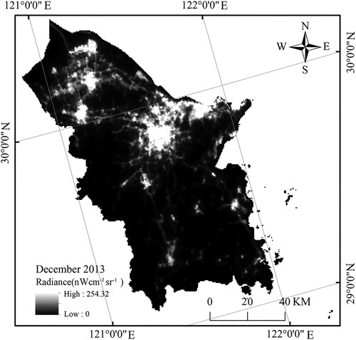
Ningbo, located at 28°51′N-30°33′N, is a prefecture-level city in Zhejiang Province located in the middle and low latitudes of the Northern Hemisphere (Figure 1). It is an important port city along the southeastern coast of China and an economic center, as approved by the State Council, abutting the southern wing of the Yangtze River Delta. As of 2021, the total area of the city was 9816 square kilometers, and as of the end of 2022, the permanent population of the city was 9.618 million. Considering the location of Ningbo in the middle and low latitudes of the Northern Hemisphere, there may be missing VIIRS nighttime light data in some months, which will greatly hinder the rapid assessment of the population and urban development level in the city based on VIIRS nighttime light data. Therefore, constructing an optimal interpolation method to obtain continuous VIIRS monthly nighttime light data for Ningbo is crucial for quickly assessing development.

Figure 1. Study area of Ningbo city.

2.2. VIIRS DNB vcm data

Monthly nighttime light data for VIIRS vcm have been produced since April 2012. In this research, data from April 2012 to December 2022 are downloaded, and the appropriate data are selected for experiments. To facilitate comparative analyses of interpolated and original images and to evaluate the accuracy of the interpolated images, the appropriate data are selected based on the completeness of VIIRS data for all months of the year. Specifically, VIIRS vcm data from the following months are selected for experimental analysis: December 2013, January-December 2014, December 2015, January-December 2016, December 2018, January-December 2019, December 2020, and January-December 2021. Select June data from 2014, 2016, 2019, and 2021 as the data to be interpolated, and use the VIIRS vcm image data from the six months before and after June to interpolate the missing June VIIRS vcm image data. The VIIRS vcm data used in this article were all downloaded from the Earth Observation Group (https://eogdata.mines.edu/products/vnl/).

3. Methods

3.1. Research framework

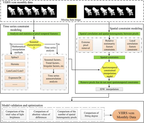
In this article, by designing a spatiotemporally comprehensive constrained interpolation model to fill missing pixel values in monthly VIIRS DNB vcm images, missing pixel values are simulated, and spatiotemporally continuous VIIIRS vcm monthly synthetic datasets are generated. The specific technical framework is shown in Figure 2.

Figure 2. Technical flowchart.

3.2. Seasonal fluctuation characteristics

To investigate whether the VIIRS vcm monthly nighttime light imagery is affected by seasonal fluctuation characteristics, a seasonal fluctuation characterization study of the VIIRS vcm monthly synthetic data is performed. A study of the seasonal fluctuation characteristics of the 2014 VIIRS DNB monthly synthetic data is carried out using the monthly VIIRS data for a total of 11 months from January 2014-May 2014 and July 2014-December 2014, and a study of the seasonal fluctuation characteristics of the 2016 VIIRS DNB monthly synthetic data is carried out using the monthly VIIRS data for a total of 11 months from January 2016-May 2016 and July 2016-December 2016. Similarly, the seasonal fluctuation characteristics of VIIRS vcm monthly synthetic data for 2019 and 2021 are studied. Two factors are used to determine whether the light brightness in the Ningbo area is characterized by obvious seasonal fluctuations: the change in the TDN in the study area in each month and the months of the maximum and minimum values of TDN in each year. The results are shown in Figure 3.

Figure 3. The total value of light brightness in Ningbo city in each month.

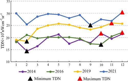
In Figure 3, the TDN in Ningbo city has no obvious seasonal fluctuation characteristics, and there is no obvious law regarding the months of the maximum and minimum values of the TDN in each year. The TDN in Ningbo city displays an increasing trend overall. Therefore, the seasonal fluctuation characteristics of images are not further considered in this paper.

3.3. Temporal interpolation method

Since there is no obvious seasonal fluctuation in light brightness in Ningbo, therefore, this article selects 8 widely used temporal interpolation methods, including Bezier3, Dr., Exponent, Hermite3, Spline3, Lsm, Lsm2, and Lsm3, for temporal interpolation modeling. The Hermite3 interpolation algorithm is implemented in MATLAB R2022a, and other interpolation algorithms are implemented in Microsoft Visual Studio 2019 using the C++ language.

The interpolation principle of Bezier curves is to define the shape of the curve through the initial and final points of the curve and the control points in the middle (Shi and Jin 2013). In this paper, the light data of two adjacent months are used as the starting and ending endpoints of the Bezier curve, and the light data of the other two months adjacent to the two months are used as the control points corresponding to the Bezier curve, and the Bezier curve is drawn according to the endpoints and control points. Due to the fact that the control points of each Bezier curve are adjacent to the starting and ending endpoints of the curve, multiple Bezier curves are smooth at adjacent intersections. The brightness values of adjacent two months’ image pixels form a Bezier curve, and the brightness data of all image pixels form a complete and smooth curve.

Dr is a simple interpolation method that considers all existing data to be accurate and replaces predicted data directly with existing data at the corresponding points. In this paper, the average value of the nighttime light brightness of pixels in May and July in each year is used to replace the nighttime light brightness value of pixels in the corresponding position in June of the corresponding year. The corresponding formula is as follows (1). (1) $P_{\mathrm{n}}^6=(P_n^5+P_n^7)/2(1\le n\le m)$(1) where $P_n^5$ is the light brightness value of the $n$th pixel in the study area in May, $P_n^7$is the light brightness value of the $n$th pixel in the study area in July, $P_n^6$ is the simulated light brightness value of the $n$th pixel in the study area in June, and $m$ is the total number of pixels in the study area.

Exponent is a method for smoothing and predicting time series data. Based on the principle of exponential smoothing, it predicts missing values based on a weighted average of existing data. The predicted value obtained by the cubic exponential smoothing method is the weighted sum of the original sequence, and the closer to the prediction time a value is obtained, the greater the corresponding weight (Zhao et al. 2017). This approach has notable advantages in short-term prediction (Wang et al. 2017) and is suitable for monthly VIIRS DNB data with unstable changes.

Hermite interpolation is one of the most commonly used methods to solve predictive problems in mathematical modeling. At a given node, it requires the function value of the interpolation polynomial to be the same as the original function value. Additionally, the derivative of the interpolation polynomial from the first order to the specified order must be equal to the derivative of the corresponding order of the interpolated function. The Hermite interpolation curve is characterized by shape preservation (Han 2018). Even if the original data are not smooth, the Hermite interpolation result will not exceed the numerical range of the original data (Fritsch and Carlson 1980).

Spline3 is a method used to approximate a set of data points through a smooth curve (Wang and Li 2015). The principle is to divide the entire dataset into multiple cells and use a cubic polynomial for interpolation within each cell so that the interpolation curve has first-order and second-order continuity at each data point. In other words, the interpolation curve passes through each data point and has the same slope and curvature. This continuity ensures the smoothness of the interpolation curve and improves the interpolation accuracy.

Least squares interpolation involves establishing a polynomial function by fitting known data points, such that the sum of squares of the distance from all data points to this function is minimized (Tian 2015). Then, the values of unknown data points are estimated based on the determined polynomial function, and the result can be used to solve the relevant interpolation and curve fitting problems.

3.4. Spatial constraint interpolation method

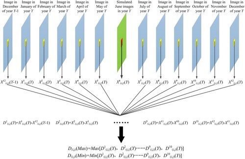
3.4.1. Constraints on the relative stability characteristics

If a country or region has not experienced serious events such as natural disasters, economic collapses, or wars, the lighting brightness in the region should not undergo significant changes in consecutive months (Zhao, Zhou, and Samson 2014). Therefore, this article presents constraints on the relative stationarity characteristics of temporal nighttime light levels, mainly from pixels with significant changes between months and pixels with significant differences between months.

Let ${\mathrm{X}}_{\left(\mathrm{i},\mathrm{j}\right)}$ represent the pixel light brightness value in row $\mathrm{i}$ and column $\mathrm{j}$ of the research area, ${\mathrm{X}}_{\left(\mathrm{i}\mathrm{j}\right)}^{\mathrm{t}}$ represent the pixel light brightness value in row $\mathrm{i}$ and column $\mathrm{j}$ in month $\mathrm{t}$, ${\mathrm{X}}_{\left(\mathrm{i}\mathrm{j}\right)}^{\mathrm{t}}\left(Y\right)$ represent the pixel light brightness value in row $\mathrm{i}$ and column $\mathrm{j}$ in month $\mathrm{t}$ of year $\mathrm{Y}$, ${\mathrm{X}}_{\left(\mathrm{i},\mathrm{j}\right)}\left(\mathrm{Max}\right)$ represent the maximum value of the pixel light brightness value in row $\mathrm{i}$ and column $\mathrm{j}$ of 12 existing images in year $\mathrm{Y}$, and ${\mathrm{X}}_{\left(\mathrm{i},\mathrm{j}\right)}\left(M\mathrm{in}\right)$ represent the minimum value of the pixel light brightness value in row $\mathrm{i}$ and column $\mathrm{j}$ of 12 existing images in year $\mathrm{Y}$. 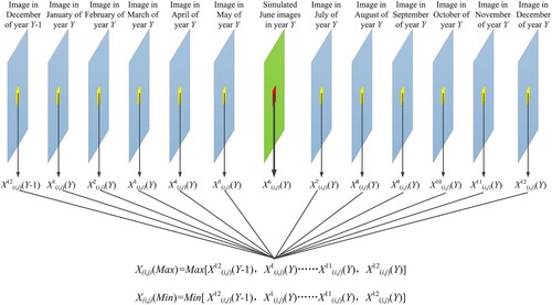If the brightness value of the pixel in row $\mathrm{i}$ and column $\mathrm{j}$ of the image simulated by the TIM in June of year $\mathrm{Y}$ is greater than${\mathrm{X}}_{\left(\mathrm{i},\mathrm{j}\right)}\left(\mathrm{Max}\right)$ or less than ${\mathrm{X}}_{\left(\mathrm{i},\mathrm{j}\right)}\left(M\mathrm{in}\right)$, this pixel is considered a pixel with significant changes between months and needs to be removed. The calculation process for pixels with drastic changes between months is shown in Figure 4.

Figure 4. The calculation process figure of dramatic change pixels in June

Let ${\mathrm{D}}_{\left(\mathrm{i},\mathrm{j}\right)}^{\mathrm{t}}\left(Y\right)$ represent the difference between the brightness values of pixels in row $\mathrm{i}$ and column $\mathrm{j}$ in month $\mathrm{t}$ of year $\mathrm{Y}$ and the brightness values of pixels in row $\mathrm{i}$ and column $\mathrm{j}$ for adjacent months.${\mathrm{D}}_{\left(\mathrm{i},\mathrm{j}\right)}\left(\mathrm{Max}\right)$ represents the maximum value of the difference in lighting brightness in row $\mathrm{i}$ and column $\mathrm{j}$ between adjacent months in year $\mathrm{Y}$, which is the upper limit of the difference.${\mathrm{D}}_{\left(\mathrm{i},\mathrm{j}\right)}\left(\mathrm{Mi}\mathrm{n}\right)$ represents the minimum value of the difference in lighting brightness in row $\mathrm{i}$ and column $\mathrm{j}$ between adjacent months in year $\mathrm{Y}$, which is the lower limit of the difference. If the difference in lighting brightness between the $\mathrm{i}$th row and $\mathrm{i}$th column pixels of the image simulated by the TIM in June of year $\mathrm{Y}$ and the corresponding position pixels of the preceding and following months is not within$[D_{(i,j)}\left(\mathrm{Min}\right)\underset{}{},D_{(i,j)}\left(\mathrm{Max}\right)]$, the pixel is considered to undergo a significant change between months and needs to be removed. The calculation process for pixels with drastic changes in monthly differences is shown in Figure 5.

Figure 5. Calculation process for pixels with dramatic changes in monthly differences.

3.4.2. Constraints on the local correlation characteristics

The first law of geography holds that the information within a spatial unit is similar to that in surrounding units, and the elements within the unit exhibit spatial autocorrelation characteristics. Spatial autocorrelation refers to the potential interdependence of observed data for certain variables within the same distribution area. The second law of geography, the law of spatial heterogeneity (Zhu et al. 2020), states that if a point’s attribute values are different from those of its surroundings, such as a hot or cold point, then that point is a spatially heterogeneous point.

Moran’s I is an important indicator used to measure spatial correlation (Liu et al. 2021). Moran’s I is further divided into global Moran’s I and local Moran’s I. For global Moran’s I, a correlation value is obtained for all elements. For local Moran’s I, a correlation value is obtained for each element. To investigate whether there is spatial autocorrelation and heterogeneity in the pixel light brightness values of VIIRS images in Ningbo city, the global Moran’s I and local Moran’s I are calculated for $3\times 3$ neighborhood pixels for all months of the study year based on VIIRS images. The calculation results are shown in Table 1 and Figure 6. notably, $\mathrm{Moran}{s}^{\mathrm{\prime }}I>0$ represents a positive spatial correlation, and the larger the value is, the more significant the spatial correlation; $\mathrm{Morans}{}^{\mathrm{\prime }}I<0$ represents a negative spatial correlation, and the smaller the value is, the greater the spatial difference. In this paper, the pixels with $\mathrm{Morans}{}^{\mathrm{\prime }}I<0$ are defined as spatial heterogeneous pixels, which need to be eliminated.

Figure 6. Local Moran’s I of the $3\times 3$ neighborhood of VIIRS images in July and August 2014.

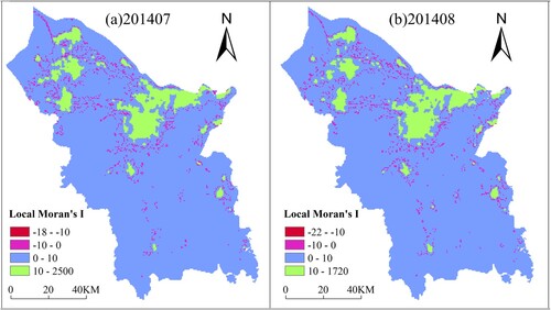
Table 1. The Global Moran’s I for each month of 2014, 2016, 2019 and 2021.

Month	Global Moran’s I in 2014	Global Moran’s I in 2016	Global Moran’s I in 2019	Global Moran’s I in 2021
January	0.892916	0.882883	0.832225	0.848658
February	0.774834	0.879178	0.849597	0.870334
March	0.873147	0.870784	0.916499	0.858178
April	0.911771	0.852261	0.907604	0.840055
May	0.852819	0.890959	0.876389	0.844779
June	0.906374	0.888372	0.89799	0.852179
July	0.877829	0.849194	0.872625	0.795484
August	0.885892	0.885693	0.889694	0.700308
September	0.90604	0.880858	0.912757	0.875363
October	0.879569	0.821109	0.833101	0.875663
November	0.870138	0.867238	0.895201	0.851655
December	0.877551	0.849684	0.899276	0.87659

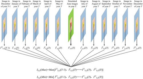
According to Table 1 and Figure 6, the VIIRS image data display obvious spatial autocorrelations. Therefore, the local correlation feature constraint modeling is carried out in this paper to better remove the abnormal pixels in the simulated images by TIM. Let ${\mathrm{I}}_{\left(\mathrm{i},\mathrm{j}\right)}$represent the $3\times 3$ neighborhood local Moran’s I of the row $\mathrm{i}$ and column $\mathrm{j}$ pixels in the study area, ${\mathrm{I}}_{\left(\mathrm{i}\mathrm{j}\right)}^{\mathrm{t}}$ represent the $3\times 3$ neighborhood local Moran’s I of the row $\mathrm{i}$ and column $\mathrm{j}$ pixels in month $\mathrm{t}$, ${\mathrm{I}}_{\left(\mathrm{i}\mathrm{j}\right)}^{\mathrm{t}}\left(Y\right)$ represent the $3\times 3$ neighborhood local Moran’s I of the row $\mathrm{i}$ and column $\mathrm{j}$ pixels in month $\mathrm{t}$ of $\mathrm{Y}$ year, ${\mathrm{I}}_{\left(\mathrm{i},\mathrm{j}\right)}\left(M\mathrm{ax}\right)$ represent the maximum value of the $3\times 3$ neighborhood local Moran’s I of the row $\mathrm{i}$ and column $\mathrm{j}$ pixels for the 12 existing images in $\mathrm{Y}$ year, and ${\mathrm{I}}_{\left(\mathrm{i},\mathrm{j}\right)}\left(M\mathrm{in}\right)$ represent the minimum value of the $3\times 3$ neighborhood local Moran’s I of the row $\mathrm{i}$ and column $\mathrm{j}$ pixels for the 12 existing images in $\mathrm{Y}$ year. If the local Moran’s I of the $3\times 3$ neighborhood of the pixels in the row $\mathrm{i}$ and column $\mathrm{j}$ image in June of year $\mathrm{Y}$ simulated with the TIM is greater than ${\mathrm{I}}_{\left(\mathrm{i},\mathrm{j}\right)}\left(\mathrm{Max}\right)$ or less than ${\mathrm{I}}_{\left(\mathrm{i},\mathrm{j}\right)}\left(M\mathrm{in}\right)$, the pixels are considered locally autocorrelated abnormal pixels and need to be eliminated. The calculation process for local autocorrelated abnormal pixels is shown in Figure 7.

Figure 7. Calculation process for locally autocorrelated abnormal pixels in a $3\times 3$ neighborhood.

3.4.3. Spatial interpolation

Relative stationarity and local correlation feature constraints based on nighttime light series are applied to the June VIIRS image data simulated by the TIM. The June VIIRS image simulated by the TIM may have missing pixels due to the removal of abnormal pixels. In this paper, the missing pixels are interpolated by the IDW method. The IDW method is a distance-based interpolation method based on the principle that things that are closer to each other are more similar than things that are farther away from each other. In the IDW method, it is assumed that each measurement point has a local influence, and this decreases as distance increases. Thus, in this method, higher weights are assigned to points closer to the predicted position. In this paper, the IDW method is used to interpolate the vacant pixels based on the pixels in the $5\times 5$ neighborhood around the vacant pixels.

4. Results

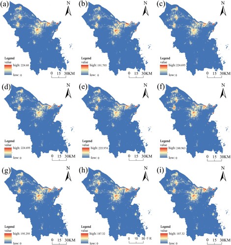
The VIIRS vcm images of Ningbo City in June 2016 simulated by TIM and SCIM are shown in Figures 8 and 9. To verify the accuracy of the TIM and SCIM constructed in this paper, an original VIIRS vcm June image was selected as the reference image. The simulated June image was compared with the original image, and the accuracy of the TIM and SCIM was evaluated from three aspects: TDN, ADN, HNP, and R².

Figure 8. Image simulated by the temporal interpolation methods (TIM). (a)Original image of June 2016 (b)Bezier3 (c)Dr (d)Exponent (e)Hermite3 (f)Spline3 (g)Lsm (h)Lsm2 (i)Lsm3.

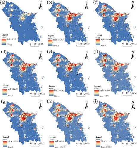
Figure 9. Image simulated by spatiotemporal comprehensive constraint interpolation method (SCIM). (a)Original image of June 2016 (b)Bezier3 (c)Dr (d)Exponent (e)Hermite3 (f)Spline3 (g)Lsm (h)Lsm2 (i)Lsm3.

4.1. Comparison of the total brightness values of lighting

The TDN of the June images simulated by the TIM and SCIM was calculated and compared with the TDN of the original June image. The results are shown in Figure 10.

Figure 10. Comparison of the total brightness values of the original image and simulated images using different methods.

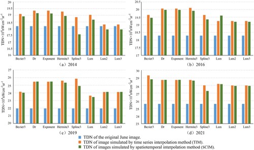
Figure 10 shows that among the eight methods used for time series interpolation, the results of the Lsm2 and Lsm3 methods are the best in 2014, 2016 and 2021, and the results of the Lsm method are the best in 2019. In 2014, the images simulated by the Dr and Exponent methods are the worst, the images simulated by the Hermite3 method are the worst in 2016, the images simulated by the Spline3 method are the worst in 2019, and the images simulated by the Bezier3 method are the worst in 2021. In summary, among the temporal interpolation methods, the Lsm2 and Lsm3 methods perform best, and all temporal interpolation methods simulate images with higher TDN than the original June image.

Comparing the accuracy of TIM and SCIM, it can be seen from Figure 10 that in 2014, except for the Lsm2 and Lsm3 methods, the TDN of images simulated by the SCIM was closer to the TDN of the original June image than the other six temporal interpolation methods; The TDN of images simulated by the SCIM in 2016, 2019, and 2021 are better than those of images simulated by the eight temporal interpolation methods. Additionally, the image simulated by the Spline3 temporal interpolation method displays the greatest improvement in image accuracy after spatiotemporal constraint interpolation, and the images simulated by the Dr and Exponent temporal interpolation methods exhibit the smallest improvement in image accuracy after spatiotemporal constraint interpolation. In summary, in terms of TDN index evaluation, the SCIM is superior to the eight selected temporal interpolation methods.

4.2. Comparison of the absolute values of differences

The ADN between the original June image pixels and the corresponding pixels of the June images simulated by the TIM and SCIM are compared. The ADN is classified into four categories: 0–1, 1–5, 5–10, and > = 10. Additionally, the number of pixels in each category is counted. The number of pixels in each ADN category for each method used in 2014, 2016, 2019, and 2021 is summed, and the results are shown in Table 2 and Table 3.

Table 2. Absolute value of the difference between the original image and images simulated with different temporal interpolation methods.

Methods	Absolute value of the difference				Average difference
	0–1	1–5	5–10	> = 10
Bezier3	123454	31840	6380	3406	0.470
Dr	125643	30380	5746	3311	0.554
Exponent	125641	30380	5749	3310	0.554
Hermite3	124345	30934	6145	3656	0.561
Spline3	119972	32615	7911	4582	0.481
Lsm	127421	30429	5118	2112	0.344
Lsm2	128939	29692	4320	2129	0.325
Lsm3	128939	29692	4320	2129	0.325

Table 3. Absolute value of the difference between the original image and the images simulated with the spatiotemporal comprehensive constraint interpolation method.

Methods	Absolute value of the difference				Average difference
	0–1	1–5	5–10	> = 10
Bezier3	123417	32034	6390	3239	0.410
Dr	125608	30455	5729	3288	0.540
Exponent	125632	30436	5729	3283	0.539
Hermite3	124636	30950	6054	3440	0.508
Spline3	122065	32096	7164	3755	0.357
Lsm	127964	30086	4946	2084	0.331
Lsm2	129270	29467	4236	2107	0.311
Lsm3	129270	29467	4236	2107	0.311

According to Tables 2 and 3, the number of pixels with AND values between 0 and 1 is the highest, and the number of pixels with ADN> = 10 is the lowest. The average AND of the corresponding position pixels between the simulated image and the original image by time series interpolation method and spatiotemporal constraint interpolation method is less than 0.57. Among the 8 temporal interpolation methods, the Lsm2 and Lsm3 interpolation methods perform the best, Spline3 method has the least number of pixels with AND between 0–1 between the simulated image and the original image, and the Hermite3 interpolation method produces the worst average ADN. For the SCIM, the Lsm2 and Lsm3 interpolation methods after considering spatiotemporal constraints perform the best, the Spline3 method after adding spatiotemporal constraints has the lowest number of pixels with ADNs between 0 and 1, and the Dr interpolation method after considering spatiotemporal constraints has the worst average ADN. At the same time, we can also find that the interpolation methods after spatiotemporal constraints provide better simulations of images than do TIM. In terms of the ADN index evaluation, the SCIM method is superior to the eight selected temporal interpolation methods.

4.3. Comparison of the number of spatially heterogeneous pixels

The local Moran’s I in the $3\times 3$ neighborhood of all image pixels in the original June image and the simulated images is calculated, and the number of image elements with negative local Moran’s I values is determined. The results are shown in Figure 11.

Figure 11. Comparison of the number of spatially heterogeneous pixels between the original image and the images simulated using different methods.

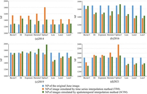
According to Figure 11, there are pixels in the original June image with a negative $3\times 3$ neighborhood local Moran’s I. Based on Figure 6, it can be roughly observed that these pixels are mostly located in the transition zone between pixels with high light brightness values and pixels with low light brightness values. The reason for the negative $3\times 3$ neighborhood local Moran’s I is the sudden decrease or increase in the light brightness values of pixels. Moreover, we find that the HNPs of the images simulated using the SCIM in 2014, 2016, 2019, and 2021 are closer to the HNPs of the original image compared to those obtained with the TIM. In terms of the HNP index evaluation, the SCIM is superior to the TIM.

4.4. Comparison of fitting degree

R² is an easy-to-calculate and very intuitive indicator for measuring the degree of fitting. The closer R² is to 1, the higher the degree of model fitting is. This paper evaluates the quality of the simulated image by calculating the R² of the TIM, SCIM simulated image and the original image. The results are shown in Table 4. At the same time, the scatter diagram of the original image and the images simulated by TIM and SCIM is drawn. The results are as follows: Figures 12 and 13.

Figure 12. Scatter plots of original image and images pixel light brightness simulated by the temporal interpolation methods (TIM) in 2014. (a)Bezier3 (b)Dr (c)Exponent (d)Hermite3 (e)Spline3 (f)Lsm (g)Lsm2 (h)Lsm3.

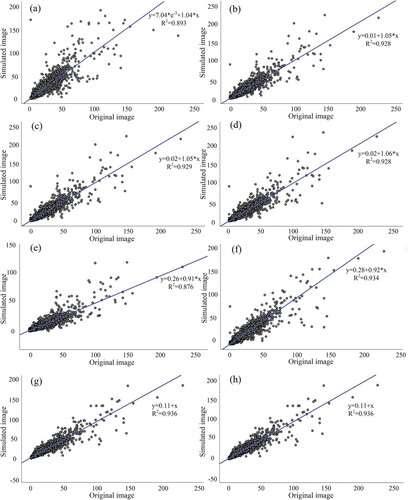
Figure 13. Scatter plots of original image and images pixel light brightness simulated by the spatiotemporal comprehensive constraint interpolation method (SCIM) in 2014. (a)Bezier3 (b)Dr (c)Exponent (d)Hermite3 (e)Spline3 (f)Lsm (g)Lsm2 (h)Lsm3.

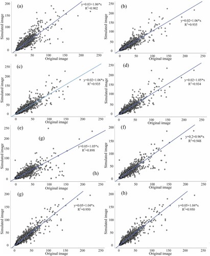
Table 4. The fitting degree (R²) between the simulated image and the original image.

R^2 between the original image and images simulated by different method	Bezier3	Dr	Exponent	Hermite3	Spline3	Lsm	Lsm2	Lsm3
TIM (2014)	0.893	0.928	0.929	0.928	0.876	0.934	0.936	0.936
SCIM (2014)	0.902	0.935	0.935	0.934	0.898	0.948	0.950	0.950
TIM (2016)	0.885	0.896	0.896	0.887	0.845	0.901	0.910	0.910
SCIM (2016)	0.897	0.906	0.906	0.908	0.881	0.907	0.916	0.916
TIM (2019)	0.907	0.915	0.915	0.907	0.889	0.923	0.931	0.931
SCIM (2019)	0.911	0.918	0.918	0.912	0.893	0.934	0.934	0.934
TIM (2021)	0.814	0.818	0.818	0.813	0.763	0.822	0.831	0.831
SCIM (2021)	0.831	0.878	0.878	0.871	0.797	0.875	0.883	0.883

From Table 4, the R² of the images simulated by SCIM and the original image are closer to 1 than the R² of the images simulated by TIM and the original image, indicating that the SCIM simulated image is closer to the original image. In the time series interpolation method and the space–time interpolation method, the R² between the image simulated by Lsm2 and Lsm3 method and the original image is the largest, and the R² between the image simulated by Spline3 method and the original image is the smallest, indicating that the June image simulated by Lsm2 and Lsm3 method is the best, and the June image simulated by Spline3 method is the worst. At the same time, it can be found that except that the R² between the image simulated by the Spline3 method and the original image in 2021 is lower than 0.8, the R² between the image simulated by other methods and the original image is higher than 0.8. The average R² between all simulated images and the original image is 0.8946, indicating that the accuracy of the images simulated by the TIM and the proposed SCIM methods is high.

5. Discussion

As one of the most widely used nighttime lighting data types, VIIRS vcm data are polluted by stray light, resulting in many missing pixels in mid- to high-latitude areas during summer. This has a very serious impact on various fields of research based on the VIIRS vcm dataset. Based on this, this article designs a spatiotemporal comprehensive constraint interpolation method that takes into account the relative stationarity of temporal night light, spatial correlation and heterogeneity between pixels. Moreover, the method considers the seasonal fluctuations in nighttime light radiation and introduces a spatial autocorrelation coefficient and spatial heterogeneity coefficient. Starting from the single-pixel scale, comprehensive analysis and verification are performed by constructing temporal feature constraints based on the relative stationarity of nighttime light patterns and local correlation feature constraints, ultimately achieving the construction of the SCIM. Extensive accuracy verifications were conducted on the images simulated by the TIM and SCIM. The results indicate that the SCIM constructed yields better TDN, ADN, NP, and R² results than the TIM for Ningbo city images.

This article takes Ningbo city as an example, and the SCIM is developed. During the construction process for this method, it was found that the monthly VIIRS vcm images of Ningbo city were not affected by seasonal fluctuation characteristics after verification, and thus, seasonal fluctuation factors were not further considered. Additionally, no verification was performed to confirm that the constructed SCIM is suitable for the interpolation of monthly missing values of VIIRS vcm data in other cities. Therefore, in future research, we will conduct research on multiple cities to analyze whether the monthly VIIRS vcm images of these cities are affected by seasonal fluctuations and to verify the applicability of the SCIM constructed in this paper.

6. Conclusion

VIIRS nighttime light data are widely used geospatial data products that reflect both the location of artificial lighting and the light intensity in an area and have high scientific research value. However, due to stray light pollution, the lack of VIIRS DNB vcm summer data is severe, which hinders the further application of VIIRS data. In this study, an SCIM that accounts for the relative stationarity of temporal nighttime light patterns and spatial correlations and heterogeneity among pixels is provided. Then, comprehensive analyses and validations are performed from three aspects: TDN, ADN, NP, and R². The conclusions are as follows:

1. Among the eight methods of temporal interpolation, the June images simulated by the Lsm2 and Lsm3 methods are best, and all the temporal interpolation methods yield images with higher TDNs than that of the original June image. The image TDNs obtained with the SCIM are closer to the TDN of the original June image than are those simulated by the TIM.

2. The number of pixels with AND values between 0 and 1 is the highest, and the number of pixels with ADN> = 10 is the lowest. The average ADN of the pixels at a corresponding position in the original image and the images simulated the TIM and SCIM is less than 0.57. The ADN of the images simulated by the temporal interpolation method with space–time constraints is better than that of the images simulated with the TIM.

3. There are spatially heterogeneous pixels in the original June image, and the HNPs in the SCIM-simulated image are closer to the HNPs in the original image than those in the TIM-simulated image.

4. The R² of the images simulated by SCIM and the original image are closer to 1 than the R² of the images simulated by TIM and the original image. The R² of the simulated image and the original image is mostly higher than 0.8, and the average R² of all simulated images and the original image is 0.8946.

In summary, the SCIM method accounts for the relative stationarity of temporal nighttime light patterns, the spatial correlations among pixels, and the heterogeneity of VIIRS DNB vcm data. The interpolation accuracy of the SCIM is higher than that of TIM interpolation. The relevant research results provide theoretical and methodological support for obtaining monthly and annual synthetic nighttime light VIIRS DNB vcm datasets with high spatiotemporal continuity and accuracy and are of great importance for improving the application of and research on nighttime light remote sensing images based on long VIIRS DNB vcm time series.

Author contributions

J.F. and Q.L. conceptualized the work. J.F. and Q.L. carried out the analytical modeling and analysis. Q.L. and J.Z. performed the nighttime light data analysis. Q.L. and Y.S. performed the land use data analysis. J.Z. and Y.S. created some graphs and tables. J.F., Q.L. and K.L. designed and conducted the experiments. J.F. and Q.L. wrote the first version of the manuscript. J.F. and J.Z. planned, coordinated, and supervised the work. All authors reviewed the manuscript.

Acknowledgments

We would like to thank the National Geophysical Data Center of the United States and the Earth Observation Group. We appreciate the editors and reviewers for their constructive comments and suggestions.

Disclosure statement

No potential conflict of interest was reported by the author(s).

Data availability statement

The data that support the findings of this study are openly available at https://eogdata.mines.edu/products/vnl/.

Additional information

Funding

This work was supported by the National Natural Science Foundation of China [grant number 42171413]; a grant from State Key Laboratory of Resources and Environmental Information System; the Shandong Provincial Natural Science Foundation [grant number ZR2020MD015 and ZR2020MD018]; the National Key Research and Development Program of China [grant number 2017YFB0503500]; and the Young Teacher Development Support Program of Shandong University of Technology [grant number 4072-115016].

References

- Chen, M. L., and H. Y. Cai. 2019. “Interpolation Methods Comparison of VIIRS/DNB Nighttime Light Monthly Composites: A Case Study of Beijing.” Progress in Geography 38 (01): 126–138. https://doi.org/10.18306/dlkxjz.2019.01.011.
- Chen, D. B., Z. H. Zheng, Z. F. Wu, and Q. L. Qian. 2019. “Review and Prospect of Application of Nighttime Light Remote Sensing Data.” Progress in Geography 38 (02): 205–223. https://doi.org/10.18306/dlkxjz.2019.02.005.
- Elvidge, C. D., K. Baugh, M. Zhizhin, F. C. Hsu, and T. Ghosh. 2017. “VIIRS Night-Time Lights International.” Journal of Remote Sensing 38 (21): 5860–5879. https://doi.org/10.1080/01431161.2017.1342050.
- Elvidge, C. D., T. Ghosh, F. C. Hsu, M. Zhizhin, and M. Bazilian. 2020. “The Dimming of Lights in China During the COVID-19 Pandemic.” Remote Sensing 12 (17): 2851. https://doi.org/10.3390/rs12172851.
- Elvidge, C. D., P. C. Sutton, T. Ghosh, B. T. Tuttle, K. E. Baugh, B. Bhaduri, and E. Bright. 2009. “A Global Poverty Map Derived from Satellite Data.” Computers & Geosciences 35 (8): 1652–1660. https://doi.org/10.1016/j.cageo.2009.01.009.
- Elvidge, C. D., M. Zhizhin, T. Ghosh, F. C. Hsu, and J. Taneja. 2021. “Annual Time Series of Global VIIRS Nighttime Lights Derived from Monthly Averages: 2012 to 2019.” Remote Sensing 13 (5): 922. https://doi.org/10.3390/rs13050922.
- Elvidge, C. D., M. Zhizhin, D. Keith, S. D. Miller, F. C. Hsu, T. Ghosh, S. J. Anderson, et al. 2022. “The VIIRS Day/Night Band: A Flicker Meter in Space?” Remote Sensing 14: 1316. https://doi.org/10.3390/rs14061316.
- Fan, J. F., H. X. He, T. Y. Hu, P. Zhang, X. Yu, and Y. K. Zhou. 2019. “Estimation of Landscape Pattern Changes in BRICS from 1992 to 2013 Using DMSP-OLS NTL Images.” Journal of the Indian Society of Remote Sensing 47 (5). https://doi.org/10.1007/s12524-019-00963-1.
- Fan, J. F., Q. Y. Liu, Z. P. Ren, Z. Chen, W. Q. Li, Y. Yu, and Y. K. Zhou. 2022. “Nighttime Luminosity Transitions are Tightly Spatiotemporally Correlated with Land Use Changes: A Pixelwise Case Study in Beijing, China.” Ecological Indicators 145: 109649. https://doi.org/10.1016/j.ecolind.2022.109649.
- Fan, J. F., T. Ma, C. H. Zhou, Y. K. Zhou, and T. Xu. 2014. “Comparative Estimation of Urban Development in China’s Cities Using Socioeconomic and DMSP/OLS Night Light Data.” Remote Sensing 6 (8): 7840–7856. https://doi.org/10.3390/rs6087840.
- Fan, J. F., P. Zhang, J. H. Chen, B. Li, L. S. Han, and Y. K. Zhou. 2020. “Quantitative Estimation of Missing Value Interpolation Methods for Suomi-NPP VIIRS/DNB Nighttime Light Monthly Composite Images.” IEEE Access 8: 199266–199288. https://doi.org/10.1109/ACCESS.2020.3035408.
- Fritsch, F. N., and R. E. Carlson. 1980. “Monotone Piecewise Cubic Interpolation.” SIAM Journal on Numerical Analysis 17 (2): 238–246. https://doi.org/10.1137/0717021.
- Gaston, K. J., J. Bennie, T. W. Davies, and J. Hopkins. 2013. “The Ecological Impacts of Nighttime Light Pollution: A Mechanistic Appraisal.” Biological Reviews 88 (4): 912–927. https://doi.org/10.1111/brv.12036.
- Guo, W., D. S. Lu, Y. L. Wu, and J. X. Zhang. 2015. “Mapping Impervious Surface Distribution with Integration of SNNP VIIRS-DNB and MODIS NDVI Data.” Remote Sensing 7 (9): 12459–12477. https://doi.org/10.3390/rs70912459.
- Han, X. 2018. “Shape-preserving Piecewise Rational Interpolation with Higher Order Continuity.” Applied Mathematics and Computation 337: 1–13. https://doi.org/10.1016/j.amc.2018.05.019.
- Imhoff, M. L., W. T. Lawrence, D. C. Lawrence, D. C. Stutzer, and C. D. Elvidge. 1997. “A Technique for Using Composite DMSP/OLS “City Lights” Satellite Data to Map Urban Area.” Remote Sensing of Environment 61 (3): 361–370. https://doi.org/10.1016/S0034-4257(97)00046-1.
- Jiang, M. D., L. Chen, Y. Q. He, X. Q. Hu, M. Q. Liu, and P. Zhang. 2022. “Nighttime Aerosol Optical Depth Retrievals from VIIRS Day/Night Band Data.” National Remote Sensing Bulletin 26 (03): 493–504. https://doi.org/10.11834/jrs.20229104.
- Levin, N. 2017. “The Impact of Seasonal Changes on Observed Nighttime Brightness from 2014 to 2015 Monthly VIIRS DNB Composites.” Remote Sensing of Environment 193: 150–164. https://doi.org/10.1016/j.rse.2017.03.003.
- Levin, N., C. C. M. Kyba, Q. Zhang, A. S. D. Miguel, and C. D. Elvidge. 2020. “Remote Sensing of Night Lights: A Review and an Outlook for the Future.” Remote Sensing of Environment 237 (C): 111443. https://doi.org/10.1016/j.rse.2019.111443.
- Li, D. R., and X. Li. 2015. “An Overview on Data Mining of Nighttime Light Remote Sensing.” Acta Geodaetica et Cartographica Sinica 44 (06): 591–601. https://doi.org/10.11947/j.AGCS.2015.20150149.
- Liu, Q. Y., J. F. Fan, Z. Chen, B. Li, and L. S. Han. 2022. “Expansion Analysis of Chengdu-Chongqing Urban Agglomeration Under Nighttime Light Remote Sensing Data Consistency Correction.” Science of Surveying and Mapping 47 (06): 99–108. https://doi.org/10.16251/j.cnki.1009-2307.2022.06.013.
- Liu, Q. Y., J. F. Fan, J. W. Zuo, P. Li, Y. P. Shen, Z. P. Ren, and Y. Zhang. 2023. “A Spatiotemporally Constrained Interpolation Method for Missing Pixel Values in the Suomi-NPP VIIRS Monthly Composite Images: Taking Shanghai as an Example.” Remote Sensing 15 (9): 2480. https://doi.org/10.3390/rs15092480.
- Liu, Z. Y., Y. Fei, H. D. Shi, L. Mo, J. X. Qi, and C. Wang. 2021. “Source Apportionment of Soil Heavy Metals in Rucheng Country of Hunan Province Based on UNMIX Model Combined with Moran Index.” Research of Environmental Sciences 34 (10): 13. https://doi.org/10.13198/j.issn.1001-6929.2021.05.25.
- Ma, T., C. H. Zhou, T. Pei, S. S. Haynie, and J. F. Fan. 2012. “Quantitative Estimation of Urbanization Dynamics Using Time Series of DMSP/OLS Nighttime Light Data: A Comparative Case Study from China’s Cities.” Remote Sensing of Environment 124. https://doi.org/10.1016/j.rse.2012.04.018.
- Ma, T., C. H. Zhou, T. Pei, S. Haynie, and J. F. Fan. 2014. “Responses of Suomi-NPP VIIRS-Derived Nighttime Lights to Socioeconomic Activity in China’s Cities.” Remote Sensing Letters 5 (2): 165–174. https://doi.org/10.1080/2150704X.2014.890758.
- Man, D. C., Tsubasa. Hirakawa, and F. K. Hiromichi. 2021. “Normalization of VIIRS DNB Images for Improved Estimation of Socioeconomic Indicators.” International Journal of Digital Earth 14 (5): 540–554. https://doi.org/10.1080/17538947.2020.1849438.
- Mills, S., S. Weiss, and C. Liang. 2013. “VIIRS Day/Night Band (DNB) Stray Light Characterization and Correction.” Proceedings of SPIE - The International Society for Optical Engineering, 8866. https://doi.org/10.1117/12.2023107.
- Shi, Y., and D. N. Jin. 2013. “Electrocardiogram Pattern Recognition Method Combining Bezier Curve Fitting.” Computer Engineering and Design 34 (04): 1437–1441. https://doi.org/10.16208/j.issn1000-7024.2013.04.011.
- Sun, G. W., M. Z. Zhang, J. F. Fan, Q. Jiang, J. H. Chen, and P. P. Zhang. 2021. “A Comparative Study on the Characteristics of the Urbanization Processes Between China and India from 1992 to 2013 Using DMSP-OLS NTL Images.” Journal of the Indian Society of Remote Sensing 49 (12): 3059–3070. https://doi.org/10.1007/s12524-021-01443-1.
- Tian, S. C. 2015. “The Least Squares Method of Statistical Principles and Applications in Agricultural Pilot Study.” Mathematics in Practice and Theory 45 (04): 124–133. https://kns.cnki.net/kcms/detail/detail.aspx?FileName=SSJS201504017&DbName=CJFQ2015
- Tveit, T., E. Skoufias, and E. Strobl. 2022. “Using VIIRS Nightlights to Estimate the Impact of the 2015 Nepal Earthquakes.” Geoenvironmental Disasters 9 (1): 1–13. https://doi.org/10.1186/s40677-021-00204-z.
- Ustaoglu, E., R. Bovkır, and A. C. Aydınoglu. 2021. “Spatial Distribution of GDP Based on Integrated NPS-VIIRS Nighttime Light and MODIS EVI Data: A Case Study of Turkey.” Environment, Development and Sustainability 23: 10309–10343. https://doi.org/10.1007/s10668-020-01058-5.
- Wang, B. B., and H. J. Li. 2015. “Temperature Compensation of Piezoresistive Pressure Sensor Based on the Interpolation of Third Order Splines.” Chinese Journal of Sensors and Actuators 28 (7). https://doi.org/10.3969/j.issn.1004-1699.2015.07.011.
- Wang, L., Q. Zhang, G. W. Huang, and J. Tian. 2017. “GPS Satellite Clock Bias Prediction Based on Exponential Smoothing Method.” Geomatics and Information Science of Wuhan University 42 (7): 995–1001. https://doi.org/10.13203/j.whugis20150089.
- Zhao, N. Z., F. C. Hsu, G. F. Cao, and E. L. Samson. 2017. “Improving Accuracy of Economic Estimations with VIIRS DNB Image Products.” International Journal of Remote Sensing 38 (21): 5899–5918. https://doi.org/10.1080/01431161.2017.1331060.
- Zhao, N. Z., Y. Y. Zhou, and E. L. Samson. 2014. “Correcting Incompatible DN Values and Geometric Errors in Nighttime Lights Time-Series Images.” IEEE Transactions on Geoscience and Remote Sensing 53 (4): 2039–2049. https://doi.org/10.1109/TGRS.2014.2352598.
- Zheng, Q. M., K. C. Seto, Y. Y. Zhou, S. X. You, and Q. H. Weng. 2023. “Nighttime Light Remote Sensing for Urban Applications: Progress, Challenges, and Prospects.” ISPRS Journal of Photogrammetry and Remote Sensing 202: 125–141. https://doi.org/10.1016/j.isprsjprs.2023.05.028.
- Zhu, A. X., G. N. Lv, C. H. Zhou, and C. Z. Qin. 2020. “Geographic Similarity: Third Law of Geography?” Journal of Geo-Information Science 22 (4): 673–679. https://doi.org/10.12082/dqxxkx.2020.200069.