A new computationally efficient algorithm to generate global fractional vegetation cover from Sentinel-2 imagery at 10 m resolution

ABSTRACT

The multi-angle method in the pixel dichotomy model (PDM) is used to produce fine spatial resolution (FSR) products of fractional vegetation cover (FVC), which involves numerous iterative computations. This phenomenon causes a low computational efficiency for global FVC. Here, we established the multi-angle equations, and simplified the two-stream approximation method to obtain multi-angle reflectance, which calculated the KDM parameters possible. Moreover, to accelerate the calculation of parameters in the multi-angle equations, land cover data were utilized as priority knowledge, which aims to decrease iterative computations to speed up the computational speed. Finally, we proposed an accelerated pixel dichotomy coupled linear kernel-driven model (PDKDM-A). By validating PDKDM-A using field measurements and FVC products, we found that the global FVC computed for various land covers exhibited strong agreement with the field measurements. The root mean square errors (RMSEs) were consistently below 0.150, except for grasslands, croplands, and cropland/natural vegetation mosaics. When comparing FVC products on the same scale, we discovered that the RMSE was less than 0.103, except for deciduous broadleaf forests. Our study demonstrates that PDKDM-A is an efficient algorithm, with the potential to quickly generate accurate global FVC products with fine spatial resolution.

KEYWORDS:

• Multi-angle method
• global FVC
• modified PDM
• high spatial resolution image
• acceleration algorithm

Nomenclature

ENF	=	Evergreen needleleaf forests
DNF	=	Deciduous needleleaf forests
MF	=	Mixed forests
OS	=	Open shrublands
S	=	Savannas
PW	=	Permanent wetlands
UBL	=	Urban and built-up lands
PSI	=	Permanent snow and ice
WB	=	Water bodies
EBF	=	Evergreen broadleaf forests
DBF	=	Deciduous broadleaf forests
CS	=	Closed shrublands
WS	=	Woody savannas
G	=	Grasslands
C	=	Croplands
CNVM	=	Cropland/natural vegetation mosaics
B	=	Barren areas
PDM	=	Pixel dichotomy model
FVC	=	Fractional vegetation cover
SMA	=	Spectral mixing analysis
FSR	=	Fine spatial resolution
VI	=	Vegetation index
NDVI	=	Normalized difference vegetation index
MODIS	=	Moderate resolution imaging spectroradiometer
IGBP-DIS	=	International Geosphere-Biosphere Program Data and Information System
RSM-LC	=	Random sampling method considering sample training of land cover
HP	=	Hemisphere photography
GBOV	=	Ground-Based Observations for Validation
MVC	=	Maximum-value composites

1. Introduction

Vegetation is a fundamental element of terrestrial ecosystems and has a significant impact on the processes of biogeochemical and hydrological cycling (Neilson 1995; Wang et al. 2017). Fractional vegetation cover (FVC) is a vegetation parameter representing the fraction of the land surface covered by green foliage in the vertical projection direction (Liang and Wang 2020; Ma et al. 2023). FVC products are utilized in vegetation research to observe worldwide phenology on both regional and global scales (Chen et al. 2016; Kang et al. 2003; Uptmoor, Pillen, and Matschegewski 2017; White, Thornton, and Running 1997). To analyze phenology at a finer scale, the estimation of FVC from fine spatial resolution (FSR) has become of high interest. Commonly employed algorithms for estimating FVC from remote sensing images consist of (a) the empirical method (Gitelson et al. 2002; Jiapaer, Chen, and Bao 2011), (b) the physical model-based technique (Chopping et al. 2012; Jia et al. 2015; Jia et al. 2016; Wang et al. 2018), (c) spectral mixing analysis (SMA) (Chang and Heinz 2000; Elmore et al. 2000; Harsanyi and Chang 1994; Jia et al. 2015; Jia et al. 2016; Okin 2007; Xiao and Moody 2005), and (d) pixel dichotomy model (PDM) method (Choudhury et al. 1994; Deardorff 1978; Gutman and Ignatov 1998; Wittich and Hansing 1995). The advantages of the algorithm need to consider computational efficiency, i.e. short computational time and high computational accuracy. When considering the combined efficiency of computational time and accuracy, the PDM proves to be more advantageous compared to other methods (Ma et al. 2023). Therefore, the PDM is appropriate for estimating FVC on both regional and global scales. The PDM utilizes the most basic formula of the normalized difference vegetation index (NDVI) to estimate FVC, given by (1) $\mathrm{FVC}={\displaystyle \frac{\mathrm{VI}-V{I}_{min}}{V{I}_{max}-V{I}_{min}},}$(1) where FVC represents the FVC, while VI_min and VI_max represent the maximum NDVI and minimum NDVI, respectively; VI denotes the re-calculated NDVI value with the image. The general form of the PDM is Equation (1). When Equation (1) is analyzed, the key parameters for calculating FVC are VI_min and VI_max.

Currently, (a) the observation data method, (b) the direct analysis method from images, and (c) the multi-angle method have become popular methods to determine VI_min and VI_max. The observation data method is carried out using ground measurement or fine-resolution products, ensuring high computational accuracy (Jiapaer, Chen, and Bao 2011; Ma et al. 2023; Zhang et al. 2013). Due to the lack of physical mechanisms, it is rarely applied to a large scale since it relies on statistical ideas to ensure the accuracy of VI_min and VI_max. To tackle this problem, the direct analysis method employs two techniques to directly obtain VI_min and VI_max from an image. One technique involves clustering analysis (Gutman and Ignatov 1998), while the other technique involves analyzing the long-term changes in land cover using a time series of VI (Zeng et al. 2000). VI_max refers to the NDVI of a scene's vegetation area that has a high leaf area index, and it can be easily acquired (Baret, Jacquemoud, and Hanocq 1993; Donohue, Roderick, and Mcvicar 2008; Ma et al. 2023). VI_min represents the NDVI of the land's ‘background’ (e.g. soil on land, sand or gravel in a desert, or gravel in the Gobi), which can be influenced by factors like components, particle size, and moisture (Ding et al. 2016). The development of the multi-angle method based on an inclined point quadrat (Wilson 1960) was a response to the considerable uncertainty in determining VI_min (Ding et al. 2016; Montandon and Small 2008). The multi-angle method utilizes the multi-angle vegetation index (VI) for the establishment of the multi-angle calculation equation. To determine VI_min and VI_max, this equation is solved using a known principle of zenith angle of 57.5° (Ma et al. 2023; Mu et al. 2018; Song et al. 2017; Song et al. 2022). The inclined point quadrat utilizes this principle, specifically, when the zenith angle is 57.5°, the multi-angle calculation equation can be solved (Baret et al. 2010; Ross 1981; Wilson 1960). When calculating FVC, the multi-angle VI is crucial for the multi-angle method. Therefore, the FSR multi-angle VI is required for the computation of FVC using FSR images. At present, the multi-angle VI is derived by the products of parameters of the linear kernel-driven model (KDM) parameters, specifically MCD43A1 (Ma et al. 2023), which is a medium-coarse spatial resolution image from the moderate resolution imaging spectroradiometer (MODIS). Most of the fine spatial resolution images are in vertical mode, obtaining the FSR multi-angle VI is challenging due to the lack of FSR multi-angle reflectance (Mu et al. 2018; Song et al. 2017). Therefore, it is crucial to determine the multi-angle reflectance by utilizing the FSR image of KDM parameters when employing the multi-angle method for calculating FSR FVC. This phenomenon has become the limitation of the PDM to expand the fine spatial resolution.

At present, there are three methods to calculate KDM parameters, i.e. (a) the fitted method from observation data, (b) the priori field method of FSR image, and (c) the radiative transfer method. The fitted method from observation data are used in the MCD43A1, it requires numerous measured reflectance to fit KDM parameters (Lucht, Schaaf, and Strahler 2000). This method considers BRDF shape from a single land cover type, ignoring the BRDF shape from heterogeneous land cover type. Therefore, the fitted method from observation data are suitable for coarse spatial resolution images with strong homogeneity, but FSR images with anisotropy have a limitation (Strugnell and Lucht 2001; Zhanqing et al. 1996). To further estimate KDM parameters from FSR images, the priori field of FSR images is proposed, which employs a moving window algorithm to invert KDM parameters from KDM (Ma et al. 2023). The moving window algorithm is suitable for estimating KDM parameters from a medium-coarse spatial resolution image on a regional scale, but it lacks computational efficiency (it cannot be computed due to numerous iterations) when estimating FSR FVC globally (Ma et al. 2023). Indeed, global FSR images of KDM parameters require a lot of memory space to pre-process. Despite the computational advantage of cloud platforms, e.g. Google Earth Engine (GEE) or PIE-Engine (Hansen et al. 2013; Teluguntla et al. 2018), it remains challenging to minimize the time in numerous iterative calculations. Therefore, the radiative transfer method is used to address this issue (Briegleb et al. 1986; Briegleb and Ramanathan 1982; Dickinson 1983; Lucht, Schaaf, and Strahler 2000). In the global scale, especially the climate model, the two-stream approximation method is used to calculate reflectance (Sellers 1985). The reflectance is calculated, which implies that can KDM parameters be calculated. However, the two-stream approximation method is still complicated in mathematical form, it is critical to simple two-stream approximation method to accelerate the algorithm.

To address the limitations of computational efficiency for the multi-angle method in estimating global FVC from FSR images, this study simplifies the two-stream approximation to calculate KDM parameters, which breaks away from the moving window algorithm and improves computational speed. Moreover, in the multi-angle method, we employ sample training of land cover to segment the global land area, consequently minimizing numerous iterative computations. Then a novel model called the accelerated pixel dichotomy coupled linear kernel-driven model (PDKDM-A) is proposed. PDKDM-A effectively expands the multi-angle method to calculate the global FVC based on FSR images.

2. Methodology

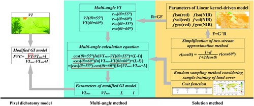
PDKDM-A is the accelerated version of the pixel dichotomy coupled linear kernel-driven model (PDKDM) (Ma et al. 2023), which is more efficient in calculating global FVC. In the PDKDM, the multi-angle equation is key in the multi-angle method, the solution of the multi-angle equation includes two components: obtaining multi-angle VI and calculation of parameters in the multi-angle equation. To obtain multi-angle VI, the KDM parameters are calculated from the FSR images. We simple two-stream approximation method to obtain multi-angle reflectance, which makes the calculation of KDM parameters possible. Moreover, to accelerate the calculation of parameters in the multi-angle equation, the land cover data are used as priority knowledge, which aims to reduce iterative computations to speed up the computational speed. The PDKDM-A is a high-speed calculation algorithm that ensures calculation accuracy, which is very suitable for the timely monitoring of FVC. Figure 1 illustrates the implementation flowchart for PDKDM-A.

Figure 1. Implementation flowchart for the accelerated pixel dichotomy method coupled with the linear kernel-driven model (PDKDM-A).

2.1. Modified pixel dichotomy model

Beer’s law-related FVC can well describe the relationship between radiation and canopy structure to represent the accurate value of FVC (Nilson 1971), the equation of Beer’s law-related FVC is: (2) $\mathrm{FVC}=1-\exp \left(-{\displaystyle \frac{{\mathrm{\Omega }}_{E}G\left({\theta }_i\right)L_{\mathrm{AI}}\left(\mathrm{VI}\right)}{\cos {\theta }_i}}\right)$(2) Here Ω_E is the clumping index. G(θ_i) represents the projection function of the area of leaves in the θ direction, which is referred to as the G function (Miller 1964; Ross 1981), L_AI (leaf area index, LAI) is a function of VI. Since the PDM ignores the radiation change due to the land's ‘background’ and the structure of the canopy in Beer’s law-related FVC, the exclusion of these factors results in certain discrepancies when estimating FVC from FSR images (Ma et al. 2023). In this study, we introduce a modified PDM to tackle deviations caused by the land ‘background’ and canopy structure, according to the derivation in Ma et al. (2023), the modified PDM is: (3) $\mathrm{FVC}={\displaystyle \frac{\mathrm{VI}\left(0^{\circ }\right)-V{I}_{min}+l}{V{I}_{max}-V{I}_{min}+L}}$(3) where l and L are that represent extensive radiation (multiple-scattering) affected by the land's ‘background’ and the structure of the canopy. VI is NDVI in this study, and it is: (4) $\mathrm{VI}={\displaystyle \frac{r_{\mathrm{NIR}}-r_{\mathrm{RED}}}{r_{\mathrm{NIR}}+r_{\mathrm{RED}}}}$(4) where r_NIR and r_RED denote the black-sky albedo in the near-infrared (NIR) and red bands, respectively. In Equation (3), VI(0°) can be obtained directly from an image. In the calculating FVC, the key parameter in the calculation of FVC include VI_min, VI_max, L, and l.

2.2. Multi-angle method

Equation (3) requires the determination of the input parameters, i.e. VI_min, VI_max, L, and l. The Beer’s law-related FVC (Equations (2)) is substituted in Equation (3), with the latter becoming: (5) $\mathrm{In}\left[{\displaystyle \frac{V_{max}-V\left({\theta }_i\right)+\left(L-l\right)}{V_{max}-V_{min}+L}}\right]=-{\displaystyle \frac{{\mathrm{\Omega }}_{E}G\left({\theta }_i\right)L}{\cos {\theta }_i}}$(5) In the inclined point quadrat method, we introduced a finding that when θ_i= 57.5°, G(θ_i) = 0.5 (Baret et al. 2010; Wilson 1960). Here θ_i is solar zenith angle. Mu et al. (2018) utilized angles of 55° and 60° to approximate 57.5° using the multi-angle method. As $G\left({57.5}^{\circ }\right)\approx G\left({55}^{\circ }\right)\approx G\left({60}^{\circ }\right)$, Equation (5) is derived as follows: (6) $\cos {55}^{\circ }\mathrm{In}\left[{\displaystyle \frac{V_{max}-V\left({55}^{\circ }\right)+\left(L-l\right)}{V_{max}-V_{min}+L}}\right]=-{\mathrm{\Omega }}_{E}G\left({55}^{\circ }\right)L$(6) (7) $\cos {60}^{\circ }\mathrm{In}\left[{\displaystyle \frac{V_{max}-V\left({60}^{\circ }\right)+\left(L-l\right)}{V_{max}-V_{min}+L}}\right]=-{\mathrm{\Omega }}_{E}G\left({60}^{\circ }\right)L$(7) Given that $G\left({57.5}^{\circ }\right)\approx G\left({55}^{\circ }\right)\approx G\left({60}^{\circ }\right)$, we have (8) $\begin{array}{rl}& \cos {55}^{\circ }\times \mathrm{In}\left[V{I}_{max}-\mathrm{VI}\left({55}^{\circ }\right)+\left(L-l\right)\right]\\ & -\cos {60}^{\circ }\times \mathrm{In}\left[V{I}_{max}-\mathrm{VI}\left({60}^{\circ }\right)+\left(L-l\right)\right]\\ & =\left(\cos {55}^{\circ }-\cos {60}^{\circ }\right)\times \mathrm{In}\left(V{I}_{max}-V{I}_{min}+L\right)\end{array}$(8) where VI(55°) and VI(60°) represent the NDVI images corresponding to solar zenith angles of 55° and 60°, respectively. The FSR images of VI(55°) and VI(60°) in Equation (8) are key for FSR FVC calculated by PDM. After obtaining FSR images of VI(55°) and VI(60°), the subsequent task involves calculating the four unidentified values in Equation (8): VI_min, VI_max, l, and L. Ultimately, based on the modified PDM, i.e. Equation (3), FVC can be calculated.

2.2.1. Acquiring multi-angle vegetation index

To calculate images of VI(55°) and VI(60°) using Eq.(3), we utilized the r_NIR and r_RED images at solar zenith angles of 55° and 60°, respectively. The images of r_NIR and r_RED at the solar zenith angles of 55° and 60° are calculated from the images of the parameters of the linear KDM, i.e. f_iso, f_vol, and f_geo (Lucht, Schaaf, and Strahler 2000). Hence, the crucial factor in determining the HSR images of VI(55°) and VI(60°) lies in obtaining FSR images of the linear KDM parameters. This study presents the introduction of the linear KDM: (9) $\begin{array}{rl}r\left({\theta }_i\right)& =f_{\mathrm{iso}}\left(g_{0\mathrm{iso}}+g_{1\mathrm{iso}}{\theta }_i^2+g_{2\mathrm{iso}}{\theta }_i^3\right)\\ & +f_{\mathrm{vol}}\left(g_{0\mathrm{vol}}+g_{1\mathrm{vol}}{\theta }_i^2+g_{2\mathrm{vol}}{\theta }_i^3\right)\\ & +f_{\mathrm{geo}}\left(g_{0\mathrm{geo}}+g_{1\mathrm{geo}}{\theta }_i^2+g_{2\mathrm{geo}}{\theta }_i^3\right)\end{array}$(9) where r(θ_i) denotes the black-sky albedo at θ_i,; and g_0iso, g_1iso, g_2iso, g_0vol, g_1vol, g_2vol, g_0geo, g_1geol, and g_2geo are polynomial coefficients of the linear KDM, whose values are presented in Table 1 (Lucht, Schaaf, and Strahler 2000).

Table 1. Polynomial coefficients in the linear kernel-driven model.

Kernel type	g0(term 1)	g1(term 2 θ)	g2(term 3 θ^2)
Isotropic	g0iso = 1	g1iso = 0	g2iso = 0
RossThick	g0vol = −0.007574	g1vol = −0.70987	g2vol = 0.307588
Lisparse-R	g0geo = −1.284909	g1geol = −1.66314	g2geo = 0.041840

Typically, a satellite with FSR images focuses primarily on vertical observation. We let the initial r(θ_i) be a reflectance image with FSR in the vertical observation. Performing an inversion of Equation (9) is necessary to calculate the FSR images for f_iso, f_vol, and f_geo. Unlike the 3 × 3 moving window that requires numerous iterative calculations, this study benefits from enhanced computational efficiency. We introduce an two-stream approximation method (alternative algorithm for the MODIS reflectance product, some study call diurnal cycle modeling) (Briegleb et al. 1986; Dickinson 1983; Liang 2004) to derive the well-posed equations (the number of equations is equal to the unknown (f_iso, f_vol, and f_geo), Equation (11)) (Briegleb et al. 1986; Briegleb and Ramanathan 1982; Lucht, Schaaf, and Strahler 2000). (10) $r\left(\cos {\theta }_i\right)={\displaystyle \frac{1+d}{1+2\mathrm{dcos}{\theta }_i}r\left(\cos {60}^{\circ }\right)}$(10) in which (11) $\begin{array}{cc}\mathrm{NDVI}\le 0.5& d=0.4\\ \mathrm{NDVI}>0.5& d=0.1\end{array}$(11) Equation (10) is a simplified version of two-stream approximation method, d in Equation (10) is obtained by the symbolic simplification in mathematics (Briegleb et al. 1986; Dickinson 1983). Equation (10) is often used in the study of radiation budget, and the relationship between the solar zenith angle and reflectance. Therefore, Equation (10) is called call diurnal cycle modeling (Liang 2004; Minnis and Harrison 1984a; 1984b). FSR images are usually vertical observations, and the solar azimuth angle (θ_i) is known. Therefore, r(cos θ_{i_1}) is a known reflectance of the FSR image, the image of r(cos θ_{i_1}) is substituted into Equation (10), and then the image of r(cos60°) can be calculated. When the image of r(cos60°) is known, Equation (10) is used to calculate the reflectance image of any angle (r(cosθ_{i_2})). Thereafter, the known image of r(cos θ_{i_1}) and two computed images of r(cos60°) and r(cosθ_{i_2}) are subjected to Equation (9), and three unknowns f_iso, f_vol, and f_geo can be established. That is, (12) $\left[\begin{array}{c}r\left(\cos {\theta }_{i\mathrm{\_}1}\right)\\ r\left(\cos {\theta }_{i\mathrm{\_}2}\right)\\ r\left(\cos {60}^{\circ }\right)\end{array}\right]=\left[\begin{array}{ccc}{g}_{\mathrm{iso}}\left({\theta }_{i\mathrm{\_}1}\right)& g_{\mathrm{vol}}\left({\theta }_{i\mathrm{\_}1}\right)& g_{\mathrm{geo}}\left({\theta }_{i\mathrm{\_}1}\right)\\ g_{\mathrm{iso}}\left({\theta }_{i\mathrm{\_}2}\right)& g_{\mathrm{vol}}\left({\theta }_{i\mathrm{\_}2}\right)& g_{\mathrm{geo}}\left({\theta }_{i\mathrm{\_}2}\right)\\ g_{\mathrm{iso}}\left({60}^{\circ }\right)& g_{\mathrm{vol}}\left({60}^{\circ }\right)& g_{\mathrm{geo}}\left({60}^{\circ }\right)\end{array}\right]\left[\begin{array}{c}{f}_{\mathrm{iso}}\\ f_{\mathrm{vol}}\\ f_{\mathrm{geo}}\end{array}\right]$(12) Equation (12) is converted to matrix-vector form and its solution is: (13) $\begin{array}{rl}& F=G^{-1}R\Rightarrow \\ & \left[\begin{array}{c}{f}_{\mathrm{iso}}\\ f_{\mathrm{vol}}\\ f_{\mathrm{geo}}\end{array}\right]=\left[\begin{array}{ccc}{g}_1& g_2& g_3\\ g_4& g_5& g_6\\ g_7& g_8& g_9\end{array}\right]\left[\begin{array}{c}r\left(\cos {\theta }_{i\mathrm{\_}1}\right)\\ r\left(\cos {\theta }_{i\mathrm{\_}2}\right)\\ r\left(\cos {60}^{\circ }\right)\end{array}\right]\end{array}$(13) Here F is the image collection composed of the f_iso image, f_vol image, and f_geo image. (14) $g_1={\displaystyle \frac{\left[g_{\mathrm{vol}}\left(60{}^{\circ }\right)g_{\mathrm{geo}}\left({\theta }_{i\mathrm{\_}2}\right)-g_{\mathrm{geo}}\left(60{}^{\circ }\right)g_{\mathrm{vol}}\left({\theta }_{i\mathrm{\_}2}\right)\right]}{g_{\mathrm{sum}}}}$(14) (15) $g_2={\displaystyle \frac{\left[g_{\mathrm{geo}}\left(60{}^{\circ }\right)g_{\mathrm{vol}}\left({\theta }_{i\mathrm{\_}1}\right)-g_{\mathrm{geo}}\left({\theta }_{i\mathrm{\_}1}\right)g_{\mathrm{vol}}\left(60{}^{\circ }\right)\right]}{g_{\mathrm{sum}}}}$(15) (16) $g_3={\displaystyle \frac{\left[g_{\mathrm{geo}}\left({\theta }_{i\mathrm{\_}1}\right)g_{\mathrm{vol}}\left({\theta }_{i\mathrm{\_}2}\right)-g_{\mathrm{vol}}\left({\theta }_{i\mathrm{\_}1}\right)g_{\mathrm{geo}}\left({\theta }_{i\mathrm{\_}2}\right)\right]}{g_{\mathrm{sum}}}}$(16) (17) $g_4={\displaystyle \frac{\left[g_{\mathrm{geo}}\left({60}^{\circ }\right)g_{\mathrm{iso}}\left({\theta }_{i\mathrm{\_}2}\right)-g_{\mathrm{iso}}\left({60}^{\circ }\right)g_{\mathrm{geo}}\left({\theta }_{i\mathrm{\_}2}\right)\right]}{g_{\mathrm{sum}}}}$(17) (18) $g_5={\displaystyle \frac{\left[g_{\mathrm{geo}}\left({\theta }_{i\mathrm{\_}1}\right)g_{\mathrm{iso}}\left({60}^{\circ }\right)-g_{\mathrm{geo}}\left({60}^{\circ }\right)g_{\mathrm{iso}}\left({\theta }_{i\mathrm{\_}1}\right)\right]}{g_{\mathrm{sum}}}}$(18) (19) $g_6={\displaystyle \frac{\left[g_{\mathrm{iso}}\left({\theta }_{i\mathrm{\_}1}\right)g_{\mathrm{geo}}\left({\theta }_{i\mathrm{\_}2}\right)-g_{\mathrm{geo}}\left({\theta }_{i\mathrm{\_}1}\right)g_{\mathrm{iso}}\left({\theta }_{i\mathrm{\_}2}\right)\right]}{g_{\mathrm{sum}}}}$(19) (20) $g_7={\displaystyle \frac{\left[g_{\mathrm{iso}}\left({60}^{\circ }\right)g_{\mathrm{vol}}\left({\theta }_{i\mathrm{\_}2}\right)-g_{\mathrm{iso}}\left({\theta }_{i\mathrm{\_}1}\right)g_{\mathrm{vol}}\left({60}^{\circ }\right)\right]}{g_{\mathrm{sum}}}}$(20) (21) $g_8={\displaystyle \frac{\left[g_{\mathrm{iso}}\left({\theta }_{i\mathrm{\_}1}\right)g_{\mathrm{vol}}\left({60}^{\circ }\right)-g_{\mathrm{iso}}\left({60}^{\circ }\right)g_{\mathrm{vol}}\left({\theta }_{i\mathrm{\_}1}\right)\right]}{g_{\mathrm{sum}}}}$(21) (22) $g_9={\displaystyle \frac{\left[g_{\mathrm{iso}}\left({\theta }_{i\mathrm{\_}2}\right)g_{\mathrm{vol}}\left({\theta }_{i\mathrm{\_}1}\right)-g_{\mathrm{iso}}\left({\theta }_{i\mathrm{\_}1}\right)g_{\mathrm{vol}}\left({\theta }_{i\mathrm{\_}2}\right)\right]}{g_{\mathrm{sum}}}}$(22)

In which (23) $g_{\mathrm{sum}}=-\left[\begin{array}{c}{g}_{\mathrm{geo}}\left({\theta }_{i\mathrm{\_}1}\right)g_{\mathrm{iso}}\left({\theta }_{i\mathrm{\_}2}\right)g_{\mathrm{vol}}\left({60}^{\circ }\right)-g_{\mathrm{geo}}\left({\theta }_{i\mathrm{\_}1}\right)g_{\mathrm{iso}}\left({60}^{\circ }\right)g_{\mathrm{vol}}\left({\theta }_{i\mathrm{\_}2}\right)\\ -g_{\mathrm{geo}}\left({\theta }_{i\mathrm{\_}2}\right)g_{\mathrm{iso}}\left({\theta }_{i\mathrm{\_}1}\right)g_{\mathrm{vol}}\left({60}^{\circ }\right)+g_{\mathrm{geo}}\left({\theta }_{i\mathrm{\_}2}\right)g_{\mathrm{iso}}\left({60}^{\circ }\right)g_{\mathrm{vol}}\left({\theta }_{i\mathrm{\_}1}\right)\\ +g_{\mathrm{geo}}\left({60}^{\circ }\right)g_{\mathrm{iso}}\left({\theta }_{i\mathrm{\_}1}\right)g_{\mathrm{vol}}\left({\theta }_{i\mathrm{\_}2}\right)-g_{\mathrm{geo}}\left({60}^{\circ }\right)g_{\mathrm{iso}}\left({\theta }_{i\mathrm{\_}2}\right)g_{\mathrm{vol}}\left({\theta }_{i\mathrm{\_}1}\right)\end{array}\right]$(23) Combining Equation (9) and Equation (23), it is possible to calculate the FSR images of VI(55°) and VI(60°). This sub-algorithm is referred to as a non-iterative algorithm.

2.2.2. Calculation of parameters associated with the modified PDM

After calculating the FSR images of VI(55°) and VI(60°), the subsequent task involves computing the four unknowns in Equation (3): VI_min, VI_max, l, and L. To determine the ranges of VI_min, VI_max, l, and L. A 3 × 3 moving window was utilized (Mu et al. 2018), whereby nine pixels in the moving window are used to establish the multi-angle calculation equations to obtain the four unknowns in the center of the moving window. Then, taking one pixel as a step, the entire image is computed through iterative calculations (Ding et al. 2016; Mu et al. 2018; Song et al. 2022). Due to the presence of numerous iterative calculations within the 3 × 3 moving window, the computational efficiency of 3 × 3 moving window algorithm is low level. We utilized a land cover dataset called DISCover from the International Geosphere-Biosphere Program Data and Information System (IGBP-DIS), as shown in Figure 3. To divide the global image into sub-images representing different classes of land cover, we employed the Monte Carlo technique to randomly acquire n reflectance values for the pixels in these sub-images, thus establishing the system of Equation (24). If the number of equations exceeds the number of unknowns, Equation (24) is an over-determined system, which only can find the optimal solution. This method is called the random sampling method considering sample training of land cover (RSM-LC), which uses the idea of distributed calculation. In a previous study by Mu et al. (2018), RSM-LC replaced the 3 × 3 moving window to solve the multi-angle calculation equation, with the following equations: (24) $\begin{array}{cc}\begin{array}{c}\cos {55}^{\circ }\times \mathrm{In}\left[V{I}_{max}-V{I}_{\left(i\right)}\left({55}^{\circ }\right)+\left(L-l\right)\right]\\ -\cos {60}^{\circ }\times \mathrm{In}\left[V{I}_{max}-V{I}_{\left(i\right)}\left({60}^{\circ }\right)+\left(L-l\right)\right]\\ =\left(\cos {55}^{\circ }-\cos {60}^{\circ }\right)\times \mathrm{In}\left(V{I}_{max}-V{I}_{min}+L\right)\end{array}& i\in \left[1,n\right]\end{array}$(24) Considering the performance of cloud computing in terms of computational speed, here we chose 10 training samples in the sub-image of each land cover class. This suggests that the quantity of equations derived from Equation (24) is greater than the unknown number. As a result, Equation (24) is an over-determined system. In the solution of this class of equations, we introduced the following cost functions to seek an optimized solution: (25) $\begin{array}{rl}& min\left\{F={\left(e{q}_1-e{q}_2\right)}^2\right\}\\ & \begin{array}{cc}\mathrm{s}.\mathrm{t}.& \mathrm{\Delta }=\left\{\left[V{I}_{max}-\mathrm{VI}\left({55}^{\circ }\right)+\left(L-l\right)\right]\ge 0\right\}\\ & \mathrm{\Delta }=\left\{\left[V{I}_{max}-\mathrm{VI}\left({60}^{\circ }\right)+\left(L-l\right)\right]\ge 0\right\}\end{array}\end{array}$(25) in which (26) $\begin{array}{rl}& e{q}_1=\cos {55}^{\circ }\times \mathrm{In}\left[V{I}_{max}-\mathrm{VI}\left({55}^{\circ }\right)+\left(L-l\right)\right]\\ & -\cos {60}^{\circ }\times \mathrm{In}\left[V{I}_{max}-\mathrm{VI}\left({60}^{\circ }\right)+\left(L-l\right)\right]\end{array}$(26) (27) $e{q}_2=\left(\cos {55}^{\circ }-\cos {60}^{\circ }\right)\times \mathrm{In}\left(V{I}_{max}-V{I}_{min}+L\right)$(27) Here VI_min, VI_max, l, and L in Equation (24) have certain physical meanings with certain value ranges referring to previous studies (Ding et al. 2016; Gutman and Ignatov 1998; Montandon and Small 2008; Mu et al. 2018). Considering the limitations of iterative computations carried out on cloud platforms, we adopted prior knowledge to obtain the value ranges of VI_min, VI_max, l, and L, as shown in Table 2.

Table 2. Value range of VI_min, VI_max, l, and L based on prior knowledge.

	Minimum	Maximum	Step
VImin	0.0	0.15	0.05
VImax	0.85	1.0	0.05
l	0	0.2	0.05
L	0	0.1	0.05

3. Validation data

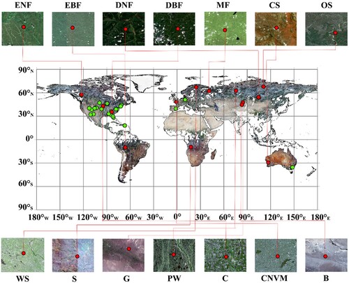
To show the performance of PDKDM-A in the estimation of global FVC, we adopted three methods: the validation with in-situ data, the validation of product data, and the comparative validation. In the field measurements, we used Copernicus Ground-Based Observations for Validation (GBOV). In the validation of product data, the FVC simulated by PDKDM-A and FVC products (PROBA-V) considering temporal and spatial variation was used to analyze the difference. In the comparative validation, we selected two common algorithms, i.e. PDKDM and radiative transfer model (PROSAIL)+back-propagation artificial neural network (BPNNs). In addition, we also used PDKDM-A to estimate monthly global FVC in 2019, and analyzed the global phenology composed of FVC. To estimate global FVC, we selected Level-2A images from Sentinel-2 with a spatial resolution of 10 × 10 m. Since Level-2A images of Sentinel-2 are surface reflectance, there was no need for any pre-processing. The cloud pixels, snow pixels and bad pixels, which influenced study on a global scale. Hence, we eliminated the snow pixel, cloud pixels and pixels of poor quality (Figure 2). The specific descriptions are shown below.

Figure 2. Synthesized Sentinel-2 images composed of RGB band on July 10th–20th, 2021. Here the field-measured plots are represented by green points, while the red points indicate the selected plots for comparing the FVC calculated by PDKDM-A with FVC products (PROBA-V). The upper and lower panels display sub-images of the areas chosen for spatial comparison between the FVC calculated by PDKDM-A and the FVC products. The land cover symbols are the same as in Figure 3. Please be aware that, because of the size, several nearby points are represented by a solitary green point.

3.1. In-situ data

We selected Copernicus Ground-Based Observations for Validation (GBOV) as the measurement source for global land products, which can be accessed at: https://land.copernicus.eu/global/gbov. The GBOV service provides high-quality, in-situ measurements across multiple years, which are widely used to validate land products, including top-of-canopy reflectance, surface albedo, fraction of absorbed photosynthetically active radiation (FAPAR), leaf area index (LAI), FVC, land surface temperature, and soil moisture. For this study, we selected the FVC between 2019 and 2020 across all locations offered by the GBOV dataset (depicted as green dots in Figure 2). These data sets are measured in 20 × 20 m plots, which use hemisphere photography (HP) or the LAI-2000 device. To comprehensively validate FVC, we first compared the different vegetation types. Subsequently, we selected several representative areas (Table 3), and compared them with the different vegetation types on time series (see Figure 3). The FVC measurements served as a benchmark for validating the FVC calculated by PDKDM-A.

Figure 3. Global land cover data in 2019.

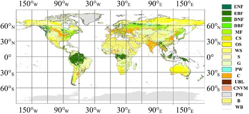
Table 3. Coordinate points for the validation of time series between the FVC calculated by PDKDM-A and field-measured data.

Land cover	Longitude	Latitude	Land cover	Longitude	Latitude
ENF	32.95070	−87.39600	EBF	17.96804	−66.86713
DBF	45.50350	−89.58731	MF	46.23430	−89.54092
CS	31.91142	−110.8375	OS	28.12833	−81.43427
G	28.12833	−81.43427	CNVM	39.57016	−1.288502

3.2. Product data of remote sensing

Currently, most FVC products comprise medium-coarse spatial resolution data, while FSR products are lacking. Hence, we performed an up-scaling procedure for the FSR FVC computed by PDKDM-A to compare it with widely utilized FVC products (Mu et al. 2015). In the choice of FVC product, we selected PROBA-V. In PROBA-V, FVC was estimated by using the machine learning algorithm from Sentinel-3 images with a spatial resolution of 300 m. This product can be accessed at https://land.copernicus.eu/global/products/fcover. To validate the accuracy of the FVC calculated by PDKDM-A in various vegetation types, we selected 14 representative sub-images from PROBA-V. The selection of these sub-images was based on the land cover data obtained from the Terra and Aqua MODIS Land Cover Type Version 6 (MCD12Q1 V6) (Figure 3). To validate the accuracy of the FVC calculated by PDKDM-A in the time series, we selected representative plots in each sub-image (red points in the sub-images in Figure 2). The coordinates of these points are shown in Table 4. Finally, the temporal and spatial PROBA-V was used as a reference FVC to validate the FVC calculated by PDKDM-A.

Table 4. Coordinate points for time series validation between the FVC calculated by PDKDM-A and PROBA-V.

Land cover	Longitude	Latitude	Land cover	Longitude	Latitude
ENF	−122.44069	57.58715	EBF	−66.23577	−10.21319
DNF	104.62585	54.20436	DBF	−83.53032	35.33409
MF	41.17381	62.08672	CS	117.13017	−29.47304
OS	110.95714	67.75252	WS	24.70378	67.17738
S	17.73188	−9.58411	G	84.50550	47.40364
PW	75.71846	62.75972	C	−94.74344	43.13848
CNVM	−0.89423	48.34098	B	83.25493	44.59965

3.3. Comparison of validated data

PDKDM-A is an accelerated version of PDKDM and PROSAIL + BPNNs has a high computational accuracy (Ma et al. 2023; Weiss and Baret 2016). Therefore, we chose these two algorithms to compare the differences between them and PDKDM-A. In the PROSAIL + BPNNs, the radiative transfer model use PROSAIL model, which assumes that the canopy is semi-infinite medium and very suitable for the crops (Jacquemoud et al. 2009; Ma et al. 2021; Verhoef 1984). PDKDM was first designed for desert vegetation (Ma et al. 2023). Therefore, the farmland and the desert were selected to analyze the differences between the two algorithms. The set of parameters in PDKDM can refer to Ma et al. (2023). The PROSAIL + BPNNs was coupled into Sentinel-2 ToolBox in the Sentinels Application Platform (SNAP) (Weiss and Baret 2016). Therefore, we used SNAP to estimate FVC. Then, FVC estimated by the PROSAILL + BPNNs was used as a ‘surrogate truth’ to validate PDKDM-A.

4. Results

4.1. Validation with in situ data

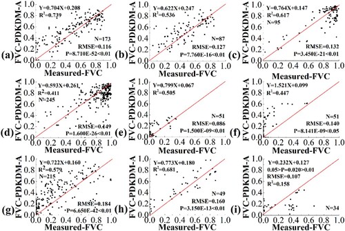
Figure 4 shows the comparison of the FVC calculated by PDKDM-A and the field-measured FVC for different land covers from 2019 to 2020. Typically, the deviations are less than 0.150, except for grasslands, croplands, and cropland/natural vegetation mosaics, which have root mean square errors (RMSEs) ranging from 0.150 to 0.20 in Figure 4(g–i). The FVC of closed shrublands estimated by PDKDM-A and the FVC products of closed shrublands show the strongest agreement in these findings (RMSE = 0.086, Figure 4(e)). The disparities between the FVC calculated by PDKDM-A and the FVC products are the most significant (Figure 4(i)). In these results, the deviation of shrubs (average RMSE = 0.113 in Figure 4(e,f)) are the smallest, followed by forests (average RMSE = 1.310 in Figure 4(a–d)) and farmland (average RMSE = 1.590 in Figure 4(h,i)), and finally grassland (average RMSE = 1.840 Figure 4(g)).

Figure 4. Comparison between the FVC calculated by PDKDM-A and field-measured FVC for different land covers. The types of forests include: (a) Evergreen needleleaf forests; (b) evergreen broadleaf forests; (c) deciduous broadleaf forests; (d) mixed forests; (e) closed shrublands; (f) open shrublands; (g) grasslands; (h) croplands; and (i) cropland/natural vegetation mosaics.

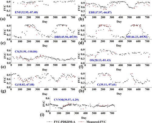
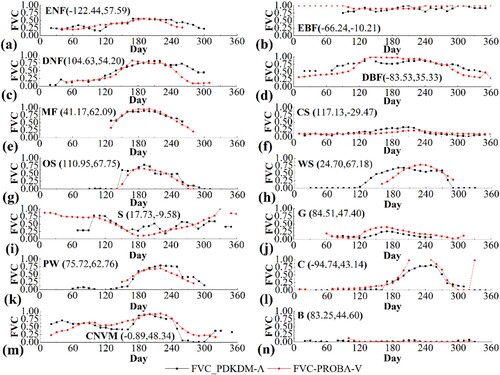
Figure 5 shows the seasonal changes between the FVC calculated by PDKDM-A and the field-measured FVC. The FVC calculated by PDKDM-A and the FVC products exhibit the highest level of consistency in relation to seasonal variations. The phenology of deciduous broadleaf forests and mixed forests is obvious, because the obvious the curve of phenology is showed in Figure 5(c,d). In Figure 5(a,b,e,i), the phenology is not particularly obvious. In grasslands, there are minor disparities in the FVC determined by PDKDM-A and the field-measured FVC (Figure 5(g)). However, the overall trend remains consistent between the two.

Figure 5. Seasonal changes were compared between the FVC calculated by PDKDM-A and the field-measured FVC for various land covers. The types of forests include: (a) Evergreen needleleaf forests; (b) evergreen broadleaf forests; (c) deciduous broadleaf forests; (d) mixed forests; (e) closed shrublands; (f) open shrublands; (g) grasslands; (h) croplands; and (i) cropland/natural vegetation mosaics. Figure 8 shows the results across a two-year period.

4.2. Comparative validation of FVC product

Figures 6–12 show the qualitative comparison among the FSR RGB image, FSR FVC estimated by PDKDM-A from Sentinel-2 images, up-scaling images for FSR FVC estimated by PDKDM-A, and FVC products (PROBA-V) in the different land covers. These results divided into seven categories, i.e. evergreen forests (Figure 6), deciduous forests (Figure 7), shrublands (Figure 8), savannas/grasslands (Figure 9), permanent wetlands (Figure 10), croplands (Figure 11) and barren areas (Figure 12). In the evergreen forests, the FVC estimated PDKDM-A in the evergreen broadleaf forests is better than that of FVC in the evergreen needleleaf forests (Figure 6). Similar phenomena also showed in Figure 13(a,b), e.g. the points in the density plots of evergreen broadleaf forests are concentrated on the 1: 1 line. In the deciduous forests, the FVC estimated by PDKDM-A in the mixed forest is the best (Figure 7(q–x)). The RMSE is 0.074 for mixed forest, which has the highest computational accuracy (Figure 13(e)). In the shrublands, the FVC of open shrublands estimated by PDKDM-A is better FVC of closed shrublands estimated by PDKDM-A (Figure 8(g,h,o,p) and Figure 13(f,g)), which implies that that PDKDM-A simulation low FVC in the shrublands have good accuracy. Similarly, the FVC of savannas estimated by PDKDM-A is better FVC of grasslands estimated by PDKDM-A, the consistency of Figure 9(w,x) is slightly different in the savannas/grasslands. In the permanent wetlands, the RMSE is 0.061 in the permanent wetlands (Figure 13(j)). Overall, the estimated FVC in the permanent wetland is still good. Finally, FVC estimated using PDKDM-A in the barren areas also has a good result (Figures 12 and 13(n)).

Figure 6. Comparing the FVC estimated using PDKDM-A with the FVC products (PROBA-V) for the evergreen forests. (a), (e), (i) and (m) are the images of needleleaf forests composed of RGB band. (b), (f), (j) and (n) are FSR FVC estimated by PDKDM-A from Sentinel-2 images. (c), (g), (k) and (o) are up-scaling images for FSR FVC estimated by PDKDM-A. (d), (h), (l), (p) are FVC products (PROBA-V). (a-h) Evergreen needleleaf forests and (i-p) evergreen broadleaf forests.

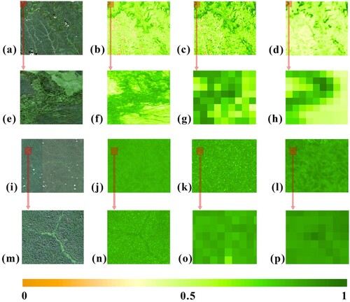
Figure 7. Comparing the FVC estimated using PDKDM-A with the FVC products (PROBA-V) for the deciduous forests. (a), (e), (i), (m), (q) and (u) are the images of deciduous forests and mixed forests composed of RGB band. (b), (f), (j), (n), (r) and (v) are FSR FVC estimated by PDKDM-A from Sentinel-2 images. (c), (g), (k), (o), (s) and (x) are up-scaling images for FSR FVC estimated by PDKDM-A. (d), (h), (l), (p), (t) and (x) are FVC products (PROBA-V). (a-h) Deciduous needleleaf forests, (i-p) deciduous broadleaf forests, and (q-x) mixed forests.

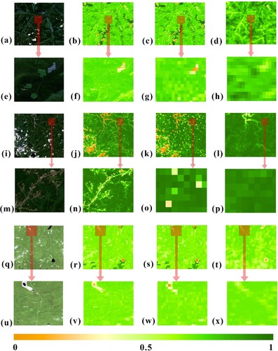
Figure 8. Comparing the FVC estimated using PDKDM-A with the FVC products (PROBA-V) for the shrublands. (a), (e), (i) and (m) are the images of shrublands composed of RGB band. (b), (f), (j) and (n) are FSR FVC estimated by PDKDM-A from Sentinel-2 images. (c), (g), (k) and (o) are up-scaling images for FSR FVC estimated by PDKDM-A. (d), (h), (l), (p) is FVC products (PROBA-V). (a-h) closed shrublands and (i-p) open shrublands.

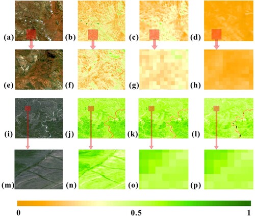
Figure 9. Comparing the FVC estimated using PDKDM-A with the FVC products (PROBA-V) for the savannas and the grasslands. (a), (e), (i), (m), (q) and (u) are the images of savannas and grasslands composed of RGB band. (b), (f), (j), (n), (r) and (v) are FSR FVC estimated by PDKDM-A from Sentinel-2 images. (c), (g), (k), (o), (s) and (x) are up-scaling images for FSR FVC estimated by PDKDM-A. (d), (h), (l), (p), (t) and (x) are FVC products (PROBA-V). (a-h) Woody savannas, (i-p) savannas, and (s-t) grasslands.

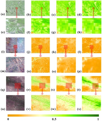
Figure 10. Comparing the FVC estimated using PDKDM-A with the FVC products (PROBA-V) for the permanent wetlands.

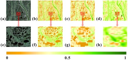
Figure 11. Comparing the FVC estimated using PDKDM-A with the FVC products (PROBA-V) for the croplands. (a), (e), (i), and (m) are the images of croplands composed of RGB band. (b), (f), (j), and (n) are FSR FVC estimated by PDKDM-A from Sentinel-2 images. (c), (g), (k), and (o) are up-scaling images for FSR FVC estimated by PDKDM-A. (d), (h), (l), and (p) are FVC products (PROBA-V). (a-h) croplands and (i-p) cropland/natural vegetation mosaics.

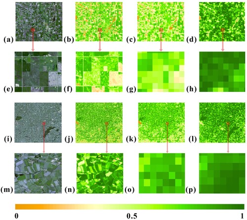
Figure 12. Comparing the FVC estimated using PDKDM-A with the FVC products (PROBA-V) for the barren areas.

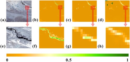
Figure 13. Density plots comparing the up-scaling images for FSR FVC estimated by PDKDM-A and FVC products (PROBA-V). Types of forests include: (a) Evergreen needleleaf forests; (b) evergreen broadleaf forests; (c) deciduous needleleaf forests; (d) deciduous broadleaf forests; (e) mixed forests; (f) closed shrublands; (g) open shrublands; (h) woody savannas; (i) savannas; (j) grasslands; (k) permanent wetlands; (l) croplands; (m) cropland/natural vegetation mosaics; and (n) barren areas.

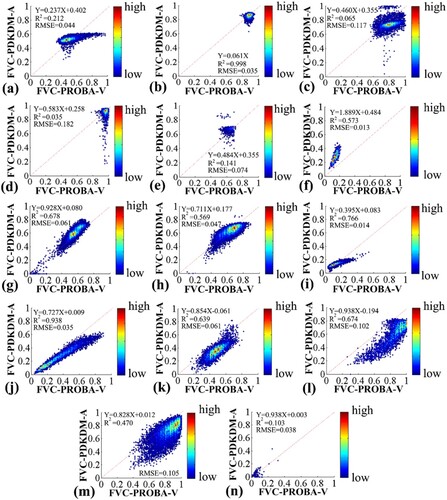
In Figures 6–7 and 13, the FVC of evergreen broadleaf forests and barren areas exhibit the highest consistency when compared to the field-measured data. In these results, there are still a few minor deviations between the FVC calculated by PDKDM-A and the FVC products for deciduous (Figure 7(a–p)) and heterogeneous vegetation landscapes (Figure 8(a–h)). Among the various types of land covers, evergreen broadleaf forests and deciduous broadleaf forests exhibit the greatest FVC, with values reaching as high as 0.900 (Figures 6 and 7). By contrast, barren areas have the lowest FVC, close to 0 (Figure 12). These results show that the accuracy of FVC estimated by PDKDM in the different land covers is different. The results of FVC calculated by PDKDM-A in the shrubs are superior to those in the grasslands, forests, and farmland, i.e. average RMSE = 0.034 in Figures 13(f–i) > RMSE = 0.035 in Figure 12(j) > average RMSE = 0.038 in Figure 13(a–e) > average RMSE = 0.104 in Figure 13(l,m). These results show that the accuracy of PDKDM in different land coverage is different.

Figure 14 shows the comparison of the FVC calculated by PDKDM-A and the FVC products in terms of seasonal changes. In these results, the FVC calculated by PDKDM-A is highly consistent with the FVC products. The FVC calculated by PDKDM-A has the highest computational accuracy in mixed forests (Figure 14(c)). The agreement between the FVC determined by PDKDM-A and the relevant FVC product is poor in closed shrublands and open shrublands, e.g. the phenology composed by FVC of closed shrublands estimated by PDKDM-A is later than that of the relevant FVC product in seasonal changes (Figure 14(f)). The FVC of open shrublands estimated by PDKDM-A exhibits a slight fluctuation in season compared to the corresponding FVC product (Figure 14(g)). In general, Figure 14 additionally shows the dynamics of vegetation growth. The growing season (SOS) begins at 120 days, while the end of the season (EOS) in the phenology occurs at 300 days, except for evergreen broadleaf forests and barren areas.

Figure 14. Comparison between the FVC calculated by PDKDM-A and FVC products (PROBA-V) in terms of seasonal changes. Types of forests include: (a) Evergreen needleleaf forests; (b) evergreen broadleaf forests; (c) deciduous needleleaf forests; (d) deciduous broadleaf forests; (e) mixed forests; (f) closed shrublands; (g) open shrublands; (h) woody savannas; (i) savannas; (j) grasslands; (k) permanent wetlands; (l) croplands; (m) cropland/natural vegetation mosaics; and (n) barren areas.

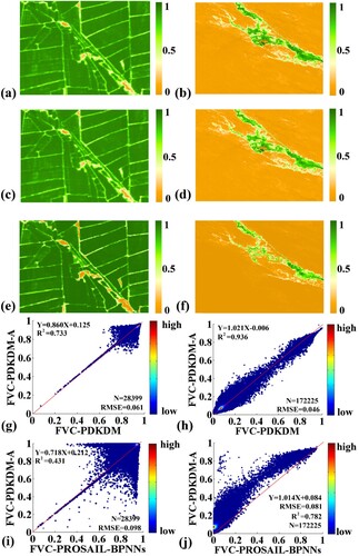
4.3. Comparative validation with PDKDM and PROSAIL + BPNNs

PDKDM-A is the accelerated version of PDKDM. Figure 15 shows the comparison results among FVC estimated by PDKDM-A and FVC estimated by PDKDM, FVC estimated by PROSAIL + BPNNs. From qualitative analysis, FVC in the croplands estimated by PDKDM-A and FVC in the croplands estimated by PDKDM have high consistency (Figure 15(a,b)). Similarly, FVC in the desert estimated by PDKDM and FVC in the desert estimated by PDKDM-A also showed higher consistency (Figure 15(c,d)). From quantitative analysis, FVC points with high density estimated by PDKDM-A and PDKDM are located on the 1: 1 line. The FVC in the croplands is above 0.9 (Figure 15(e)), and the FVC in the desert area is below 0.1 (Figure 15(f)). The difference between the FVC estimate by PDKDM-A and that of the estimate by PDKDM is less than 0.062, i.e. RMSE = 0.061 in Figure 15(e) and RMSE = 0.046 in Figure 15(f). Similarly, FVC estimated by PDKDM-A and FVC estimated by BPNNs also show the high consistency, but there are slight differences in the desert (Figure 15(j)). FVC estimated by BPNNs is slightly lower than FVC estimated by PDKDM-A, especially the especially between 0.2 and 0.8 in the FVC. The total deviation is not obvious (RMSE < 0.782). These results imply that the calculation accuracy among PDKDM-A, PDKDM, PROSAIL + BPNNs is very close, and the PDKDM-A accelerates the computational speed while ensuring a certain accuracy.

Figure 15. Comparison between FVC estimated by PDKDM and FVC estimated by PDKDM-A. (a) FVC in the croplands estimated by PDKDM, (b) Croplands FVC estimated by PDKDM-A, (c) FVC in the desert estimated by PDKDM, (d) FVC in the desert estimated by PDKDM-A, (e) FVC in the croplands estimated by PROSAIL + BPNNs in the Sentinel-2 ToolBox, (f) Croplands FVC estimated by PROSAIL + BPNNs in the Sentinel-2 ToolBox, (g) density plots comparing the FVC in the croplands calculated by PDKDM and PDKDM-A, (h) density plots comparing the FVC in the desert calculated by PROSAIL + PDKDM and PDKDM-A. (i) density plots comparing the FVC in the croplands calculated by PROSAIL + BPNNs and PDKDM-A, (j) density plots comparing the FVC in the desert calculated by BPNNs and PDKDM-A.

4.4. Change in fractional vegetation cover

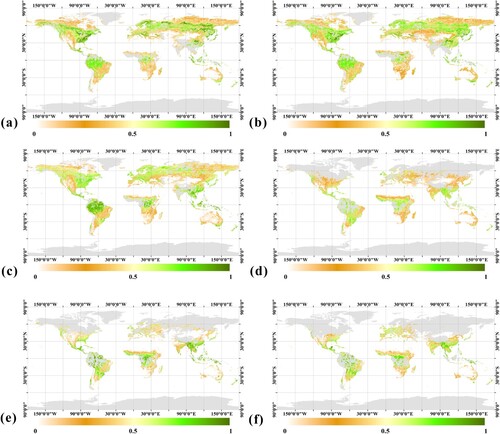
Figures 16 and 17 show the global FVC calculated by PDKDM-A in 2019 used valid pixels; these FVC data have a spatial resolution of 10 m and a time resolution of 1 month. At 60°N, the gray transforms to yellow, then green, and finally back to gray. The gray indicates that there are no high-quality pixels at 60°N from January-April and November to December. The main reason is that the snow pixel was removed in the pre-processing. Analyzing the land cover data in Figure 3, 60°N corresponds to deciduous broadleaf forests and mixed forests, which are boreal coniferous forests. These results demonstrate that the changes in the FVC of boreal coniferous forests at 60°N are the most significant in the phenology. The area of maximum value of the FVC and the peak of FVC during the phenological stage of growth is in July (Figure 17(a)). After July, this FVC gradually decreases. In addition, the seasonal changes in the FVC of tropical rainforests (near the Equator) are not significant (green area in Figures 16 and 17). In Figures 16 and 17, the gray area is very large in tropical rainforests, indicating FSR images are lack in this area. In the temperate zone, the FVC on the west coast of the mainland (an area controlled by subpolar westerlies) and the east coast of the mainland (an area controlled by a monsoon) changes with the season, the Northern Hemisphere becoming green, and the Southern Hemisphere becoming yellow. In the Arctic Circle, the map shows gray in January and December, which further indicates that most of this area is covered with snow and ice currently. In general, PDKDM simulates the change of FVC in the global vegetation.

Figure 16. Global FVC with a spatial resolution of 10 m and a time resolution of 1 month in the first half of 2019. The months of the year are: (a) January; (b) February; (c) March; (d) April; (e) May; (f) June.

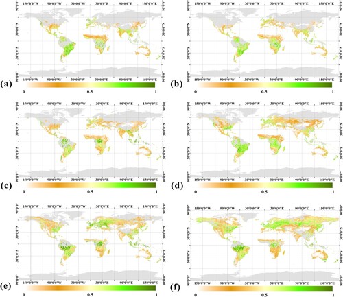
Figure 17. Global FVC with a spatial resolution of 10 m and a time resolution of 1 month in the second half of 2019. The months of the year are: (a) July; (b) August; (c) September; (d) October; (e) November; and (f) December.

Furthermore, in terms of computational time, PDKDM-A requires less time for the calculation of the global FVC (approximately two minutes as shown in Table 5). This suggests that the algorithm successfully accomplishes its objective of being computationally efficient. Because the pixels in the image are influenced by clouds, snow, and quality, snow pixels, cloud pixels and poor-quality pixels are removed in pre-processing. Like phenology, the valid pixel changes with the seasons, which presented a form of cosine function in 2019. The valid pixels are the highest in July, it can be close to 80% (Figure 18(a)). The reason for this is that there are differences in the land area of the two hemispheres of the north and south. Although many tropical areas are influenced by clouds and snow, it has caused less valid pixels. From the valid pixels, FVC <25% is the largest, which is changed by season (Figure 18(b)). These results also imply that the large area of global land is still mainly low FVC.

Figure 18. Proportion of valid pixel for FVC and FVC in the different levels for valid pixels. (a) Proportion of valid pixels for the estimation of FVC in land surface area, (b) FVC in the different levels for the valid pixels of the estimation of FVC in land surface area.

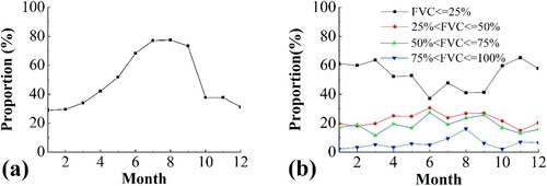
Table 5. Computational time statistics of PDKDM-A for global FVC with a spatial resolution of 10 m and a time resolution of 1 month.

Month	Time (second)	Month	Time (second)
January	113	February	117
March	121	April	147
May	143	June	135
July	177	August	160
September	128	October	141
November	114	December	158

Note: PDKDM-A was implemented using Google Earth Engine.

5. Discussion

5.1. Advantages of PDKDM-A in terms of calculation efficiency

The empirical method, the physical model-based technique, the SMA, and PDM are the most commonly methods at present (Ma et al. 2023; Mu et al. 2018). The experience method usually has high calculation accuracy on a small scale, which rarely is used to calculate global FVC due to lack of physical mechanism. The physical model-based technique is used to calculate the global FVC. The physical model-based technique usually involves machine learning, which needs to produce a dataset by physical model and retrieval FVC from pixel by pixel. Therefore, the physical model-based technique is used to calculate the global FVC which costs a lot of time. The SMA and PDM are a good choice considering computational efficiency. However, SMA involves the complex matrix to solve the linear equation system, which increases mathematics complexity to calculate global FVC. Compared with SMA, PDM is an algorithm with low mathematical complexity and high computational efficiency. Therefore, it is very suitable for the calculation of global FVC.

In PDM, the parameters in the PDM or modified PDM (Equation (1) or Equation (3)) are key. Multi-VI used 3 × 3 moving window algorithms to calculate the parameters (VI_min and VI_max in Equation (1)) of each pixel in the PDM (Mu et al. 2018). The calculation speed of Multi-VI is very slow. Therefore, PDM was modified to modified PDM considering the radiation change. 3 × 3 moving window algorithms were further modified to chessboard block + Monte Carlo method to calculate the parameters (VI_min, VI_max, l, and L in Equation (3)) of the chessboard area in the modified PDM. The pixel dichotomy coupled linear kernel-driven model (PDKDM) was proposed to estimate FVC (Ma et al. 2023). However, for the inversion of global FVC from the FSR image, this improvement in the PDKDM is not perfect. Because the calculation of global FVC involved numerous pixels. Based on a certain calculation accuracy, PDKDM needs to be further optimized to accelerate the computational speed.

In this study, we attempted to simplify the large amount of iterative calculation required in the multi-angle method. Then, PDKDM-A was proposed. PDKDM-A employed RSM-LC to calculate the parameters (VI_min, VI_max, l, and L in Equation (3)) of land cover in the modified PDM (Section 2.2.2). The innovation of computational speed makes PDKDM-A calculate the global FVC in only about 2 minutes based on GEE (see Table 5), which implies that PDKDM-A has an advantage in the computational time. In this study, PDKDM-A demonstrated a quick computational speed while maintaining the high accuracy in the calculations (RMSE < 0.062 in Figure 15). For instance, the differences between the FVC calculated by PDKDM-A and the measured FVC were generally less than 0.150, except for grasslands, croplands, and cropland/natural vegetation mosaics, where the RMSEs ranged from 0.150 to 0.200 as shown in Figure 4(g–i). In addition, the FVC calculated by PDKDM-A demonstrated considerable consistency with the applicable FVC product, e.g. the difference between the FVC calculated by PDKDM-A and the relevant FVC product was less than 0.100 for most land covers (Figure 13(a,b,e–k,n), although there were some exceptions (Figure 5(c,d,l,m)). Therefore, given its comprehensive calculation efficiency (based on its computational accuracy and the time it requires), PDKDM-A can be considered an excellent algorithm suitable for estimating global FVC.

5.2. Algorithm design of advantages and improvement in PDKDM-A

Most FSR satellites are obtained from vertical mode, and the reflectance of the pixels in the images is also a variable of vertical direction. Therefore, the NDVI calculated by such reflectance is also variable in the vertical direction. In PDKDM-A, to calculate FSR FVC, the modified PDM needs to be solved. Therefore, the four parameters in Equation (3) are required: VI_min, VI_max, l, and L. To solve these four parameters applied to the FSR issue, the inversion of linear KDM (Equations (10)–(23)) is key. In PDKDM, the iterative algorithm with a 2 × 2 moving window is used (Ma et al. 2023). In this algorithm, four pixels can be calculated at one time to solve an overdetermined system, i.e. the number of equations is greater than the number of unknowns, Equation (B-6) in Ma et al. (2023). Therefore, the computational speed of the entire image is very slow. In this study, we introduced a simplified version of the two-stream approximation method to establish a mathematical relationship between the vertical reflectance and the reflectance at various angles (Equation (10)). Then, well-posed equations were established to avoid iteration calculation to calculate the image at one time. Because most FSR satellites are mostly vertical modes, Equation (10) is used to imply that we can calculate other angle reflectance based on vertical reflectance. The above two technological breakthroughs make the FSR global FVC rapid calculation possible.

The estimation of global FVC from FSR images using the multi-angle method has been infrequently employed in prior studies. In response, we have constituted an attempt to apply this method to estimate global FVC from FSR images. PDKDM-A is the new multi-angle method in the PDM. While PDKDM-A has the capability to compute global FVC using FSR images, these images are susceptible to the influence of cloud pixels and bad pixels (Gray in Figures 16 and 17). In contrast to medium-coarse space resolution images, FSR images cover small scenes in the land. Therefore, several pixels are lost in the medium-coarse spatial resolution, which in turn means that dozens of FSR images are lost, too, resulting in the enduring and serious issue of discontinuous FVC. The number of high-quality pixels is less than 80% of the land surface area (Figure 18(a)). When the sun is located southern hemisphere from November to February, many land areas in the northern hemisphere have snow and rain in winter (Gray and white in Figure 16(a–b) and Figure 17(e–f)). Therefore, the number of high-quality is less from November to February than in other months (Figure 18(a)). In addition, the most of the global FVC is less than 0.25 in the valid pixels (Figure 18(a)), the tropical rainforest has a thicker cloud, which leads to a lack of valid pixels. This phenomenon further implies that most of the global vegetation is in a dry state.

In previous studies, a method based on the PROSAIL + BPNNs is gathered in Sentinel-2 ToolBox to estimate FVC from Sentinel-2 (Weiss and Baret 2016). A learning dataset was generated based on the PROSAIL. The pre-processing is very troublesome, which results in the computational time being very slow. Therefore, the FVC estimated by Sentinel-2 ToolBox from Sentinel-2 image only be applied to a small scale and it is hard to be apply the fast estimate of FVC on a global scale. In addition, the difference of FVC is between 0.2 and 0.8 estimated by PDKDM-A and PROSAIL + BPNNs, because the learning dataset required by BPNNs was produced based on the PROSAIL model. The PROSAIL model assumes that the canopy is semi-infinite medium, which is very suitable for crops, and it is not suitable for deserted vegetation (Jacquemoud et al. 2009; Verhoef 1984). Therefore, there are slight differences in the desert (Figure 15(j)). However, in the study by Weiss and Baret (2016), the characterization of the heterogeneity of the pixel environment needs to be considered in the fusion algorithm of time and space. In the future, we will study this issue and propose a fusion algorithm of time and space (Feng et al. 2006; Hilker et al. 2009; Li et al. 2017, 2020; Wang et al. 2021; Zhang et al. 2018; Zhu et al. 2010) to repair the FSR FVC products.

5.3. Accuracy of FVC in different land cover

Our algorithm is very suitable for estimating heterogeneous canopies in different land covers. The calculation accuracy of shrublands estimated by PDKDM-A is high when compared to grasslands, forests, and farmland. This includes closed shrublands, open shrublands, woody savannas, and savannas in Figure 13(f–i) (mean RMSE = 0.034) and Figure 4(e,f) (mean RMSE = 0.107). The primary reason is that our algorithm is based on the PDM, which was developed to account for mixed scenes composed of vegetation and ‘background.’ Such mixed scenes are like heterogeneous canopies. Furthermore, to improve the physical mechanism in our modeling, we utilize the graphical method to modify the PDM considering radiation changes caused by the canopy structure and land ‘background’ (L and l in (Ma et al. 2023)). The accuracy of calculating the FVC of shrublands was further enhanced by this treatment. Figure 14 shows that the precision of grasslands and forests was slightly lower compared to shrublands, but still less than 0.185, specifically with a mean RMSE of 0.035 in grasslands see Figure 14(j); RMSE = 0.184 in grasslands, see Figure 4(g); mean RMSE  = 0.038 in forests, see Figure 7(a–e); and mean RMSE = 0.130 in forests, see Figure 4(a–d). Therefore, the FVC calculated by PDKDM-A exhibited high calculation accuracy in shrublands, grasslands, and forests. The PDKDM-A can be used to estimate the FVC for most major vegetation types. Analyzing Figure 3, one can see that 90% of the vegetation at the global scale comprises shrubs, grasslands, and forests.

Additionally, the accuracy of PDKDM-A will decrease when FVC with non-green leaves was estimated. This phenomenon is particularly obvious in the FVCs of croplands, see Figure 4(i) and Figure 14(l,m). In the heading-flowering period, some colorful flowers of wheat open (July 10th–20th in Figure 2). Compared with FVC with green leaves, the accuracy of FVC with non-green leaves is lower (RMSE = 0.102 in Figure 4(i)). The primary reason is that our algorithm is affiliated with PDM, which was designed and developed based the NDVI. NDVI is designed by red band and near-infrared band, which recognizes is relatively poor in the non-green leaves. PDMs developed based on this index, which is established based on the green leaves. Therefore, modified PDM has computational deviation to estimate FVC. The non-green canopy is less widely distributed across the world; hence it can be ignored from the estimation of global FVC.

Moreover, to speed up the computational speed, we have considered priority knowledge to reduce the dataset generated from the range of parameters of the modified PDM (VI_min, VI_max, l, and L). Compared with PDKDM, the loss of calculation accuracy of PDKDM-A is not obvious (Figure 15(e,f)). Considering the computational speed, this study directly uses the dataset of land cover coupled in the cloud platform, i.e. MCD12Q1 V6 (Figure 3). MCD12Q1 V6 is the product of land cover with a spatial resolution of 500 m. The spatial resolution between MCD12Q1 V6 and FVC estimated by PDKDM-A is inconsistent, which is also the source of computational deviation. However, MCD12Q1 V6 is coupled to the cloud platform, which makes the computational process more convenient. Considering the computational time and computational accuracy, the dataset coupled in the cloud platform is the best choice.

6. Conclusion

In addition to computational accuracy, the computational speed is also very important in the inversion of remote sensing. In this study, based on the PDKDM, we introduced the two-stream approximation method and RSM-LC to quickly solve the multi-angle equation, and proposed a PDKDM-A aimed at reducing the iteration calculations in the previous multi-angle method. We validated the method using field-measured data and a comparison of validated data. The FVC calculated by PDKDM-A demonstrated high accuracy when compared to the data measured in the field. Furthermore, we identified a high level of consistency between the FVC calculated by PDKDM and FVC products. These results show that PDKDM-A can be successfully applied to estimate global FVC and has the capability to estimate FVC due to its remarkable calculation efficiency. PDKDM-A is implemented on the Google Earth Engine (https://code.earthengine.google.com/9f46a5a1a8a7f8496f07f40096dfeea8), which can quickly calculate the global FVC and provide an important tool for the real-time monitoring of the vegetation.

Acknowledgements

The authors appreciate the editors and anonymous reviewers for their valuable suggestions.

Disclosure statement

No potential conflict of interest was reported by the author(s).

Data availability statement

The data supporting the findings of this study are estimated from the Google Earth Engine. Restrictions apply to the availability of these data, which were used under the license for this study. Data are available from the author, [email protected].

Correction Statement

This article has been corrected with minor changes. These changes do not impact the academic content of the article.

Additional information

Funding

This study was supported in part by the National Natural Science Foundation of China [grant number 42201390], in part by the University of Basic Scientific Business Fees for Scientific Research Projects in the Xinjiang Uygur Autonomous Region [grant number XJEDU2022P014]; in part by the Ph.D. Starts Funds, Xinjiang University [grant number 620321021]; in part by the Postdoctoral Research Foundation of China [grant number 2021M702748]; in part by the Open Project of Key Laboratory in the Xinjiang Uygur Autonomous Region [grant number 2023D04051]; in part by the Tianchi Doctoral Program in the Xinjiang Uygur Autonomous Region [grant number TCBS202127]; in part by the International Cooperation Scientific Research Project of the Ministry of Education ‘Chunhui Plan’ [grant number HZKY20220609]; in part by the State Key Laboratory of Desert and Oasis Ecology, Xinjiang Institute of Ecology and Geography, Chinese Academy of Sciences [grant number G2023-02-05], General Project of the Central Asian Research Institute from Xinjiang University [grant number 24FPY003].

References

- Baret, F., B. de Solan, R. Lopez-Lozano, K. Ma, and M. Weiss. 2010. “GAI Estimates of Row Crops from Downward Looking Digital Photos Taken Perpendicular to Rows at 57.5° Zenith Angle: Theoretical Considerations Based on 3D Architecture Models and Application to Wheat Crops.” Agricultural and Forest Meteorology 150: 1393–1401. https://doi.org/10.1016/j.agrformet.2010.04.011.
- Baret, F., S. Jacquemoud, and J.-F. Hanocq. 1993. “The Soil Line Concept in Remote Sensing.” Remote Sensing Reviews 13: 281–284.
- Briegleb, B. P., P. Minnis, V. Ramanathan, and E. Harrison. 1986. “Comparison of Regional Clear-Sky Albedos Inferred from Satellite Observations and Model Computations.” Journal of Climate and Applied Meteorology 25: 214–226. https://doi.org/10.1175/1520-0450(1986)025<0214:CORCSA>2.0.CO;2.
- Briegleb, B., and V. Ramanathan. 1982. “Spectral and Diurnal Variations in Clear Sky Planetary Albedo.” Journal of Applied Meteorology 21: 1160–1171. https://doi.org/10.1175/1520-0450(1982)021<1160:SADVIC>2.0.CO;2.
- Chang, C.-I., and D. C. Heinz. 2000. “Constrained Subpixel Target Detection for Remotely Sensed Imagery.” IEEE Transactions on Geoscience and Remote Sensing 38: 1144–1159. https://doi.org/10.1109/36.843007.
- Chen, M., E. K. Melaas, J. M. Gray, M. A. Friedl, and A. D. Richardson. 2016. A New Seasonal-Deciduous Spring Phenology Submodel in the Community Land Model 4.5: Impacts on Carbon and Water Cycling Under Future Climate Scenarios. Global Change Biology.
- Chopping, M., M. North, J. Chen, C. B. Schaaf, J. B. Blair, J. V. Martonchik, and M. A. Bull. 2012. “Forest Canopy Cover and Height from MISR in Topographically Complex Southwestern US Landscapes Assessed with High Quality Reference Data.” IEEE Journal of Selected Topics in Applied Earth Observations and Remote Sensing 5: 44–58. https://doi.org/10.1109/JSTARS.2012.2184270.
- Choudhury, B. J., N. U. Ahmed, S. B. Idso, R. J. Reginato, and C. S. T. Daughtry. 1994. “Relations Between Evaporation Coefficients and Vegetation Indices Studied by Model Simulations.” Remote Sensing of Environment 50: 1–17. https://doi.org/10.1016/0034-4257(94)90090-6.
- Deardorff, J. W. 1978. “Efficient Prediction of Ground Surface Temperature and Moisture with Inclusion of a Layer of Vegetation.” Journal of Geophysical Research: Oceans 83: 1889–1903. https://doi.org/10.1029/JC083iC04p01889.
- Dickinson, R. E. 1983. “Land Surface Processes and Climate—Surface Albedos and Energy Balance.” In Advances in Geophysics, edited by B. Saltzman, 305–353. Amsterdam: Elsevier.
- Ding, Y., X. Zheng, K. Zhao, X. Xin, and H. Liu. 2016. “Quantifying the Impact of NDVIsoil Determination Methods and NDVIsoil Variability on the Estimation of Fractional Vegetation Cover in Northeast China.” Remote Sensing 8: 29. https://doi.org/10.3390/rs8010029.
- Donohue, R. J., M. L. Roderick, and T. R. Mcvicar. 2008. “Deriving Consistent Long-Term Vegetation Information from AVHRR Reflectance Data Using a Cover-Triangle-Based Framework.” Remote Sensing of Environment 112: 2938–2949. https://doi.org/10.1016/j.rse.2008.02.008.
- Elmore, A. J., J. F. Mustard, S. J. Manning, and D. B. Lobell. 2000. “Quantifying Vegetation Change in Semiarid Environments: Precision and Accuracy of Spectral Mixture Analysis and the Normalized Difference Vegetation Index.” Remote Sensing of Environment 73: 87–102. https://doi.org/10.1016/S0034-4257(00)00100-0.
- Feng, G., J. G. Masek, M. R. Schwaller, and F. F. Hall. 2006. “On the Blending of the Landsat and MODIS Surface Reflectance: Predicting Daily Landsat Surface Reflectance.” IEEE Transactions on Geoscience and Remote Sensing 44: 2207–2218. https://doi.org/10.1109/TGRS.2006.872081.
- Gitelson, A. A., Y. J. Kaufman, R. Stark, and D. Rundquist. 2002. “Novel Algorithms for Remote Estimation of Vegetation Fraction.” Remote Sensing of Environment 80: 76–87. https://doi.org/10.1016/S0034-4257(01)00289-9.
- Gutman, G., and A. Ignatov. 1998. “The Derivation of the Green Vegetation Fraction from NOAA/AVHRR Data for Use in Numerical Weather Prediction Models.” International Journal of Remote Sensing 19: 1533–1543. https://doi.org/10.1080/014311698215333.
- Hansen, M. C., P. V. Potapov, R. Moore, M. Hancher, S. A. Turubanova, A. Tyukavina, D. Thau, et al. 2013. “High-Resolution Global Maps of 21st-Century Forest Cover Change.” Science 342: 850–853. https://doi.org/10.1126/science.1244693.
- Harsanyi, J. C., and C. I. Chang. 1994. “Hyperspectral Image Classification and Dimensionality Reduction: An Orthogonal Subspace Projection Approach.” IEEE Transactions on Geoscience and Remote Sensing 32: 779–785. https://doi.org/10.1109/36.298007.
- Hilker, T., M. A. Wulder, N. C. Coops, J. Linke, G. Mcdermid, J. G. Masek, G. Feng, and J. C. White. 2009. “A New Data Fusion Model for High Spatial- and Temporal-Resolution Mapping of Forest Disturbance Based on Landsat and MODIS.” Remote Sensing of Environment 113: 1613–1627. https://doi.org/10.1016/j.rse.2009.03.007.
- Jacquemoud, S., W. Verhoef, F. Baret, C. Bacour, P. J. Zarco-Tejada, G. P. Asner, C. François, and S. L. Ustin. 2009. “PROSPECT+SAIL Models: A Review of Use for Vegetation Characterization.” Remote Sensing of Environment 113: S56–S66. https://doi.org/10.1016/j.rse.2008.01.026.
- Jia, K., S. Liang, X. Gu, F. Baret, X. Wei, X. Wang, Y. Yao, L. Yang, and Y. Li. 2016. “Fractional Vegetation Cover Estimation Algorithm for Chinese GF-1 Wide Field View Data.” Remote Sensing of Environment 177: 184–191. https://doi.org/10.1016/j.rse.2016.02.019.
- Jia, K., S. Liang, S. Liu, Y. Li, Z. Xiao, Y. Yao, B. Jiang, et al. 2015. “Global Land Surface Fractional Vegetation Cover Estimation Using General Regression Neural Networks from MODIS Surface Reflectance.” IEEE Transactions on Geoscience and Remote Sensing 53: 4787–4796. https://doi.org/10.1109/TGRS.2015.2409563.
- Jiapaer, G., X. Chen, and A. Bao. 2011. “A Comparison of Methods for Estimating Fractional Vegetation Cover in Arid Regions.” Agricultural and Forest Meteorology 151: 1698–1710. https://doi.org/10.1016/j.agrformet.2011.07.004.
- Kang, S., S. W. Running, J. H. Lim, M. Zhao, C. R. Park, and R. Loehman. 2003. “A Regional Phenology Model for Detecting Onset of Greenness in Temperate Mixed Forests, Korea: An Application of MODIS Leaf Area Index.” Remote Sensing of Environment 86: 232–242. https://doi.org/10.1016/S0034-4257(03)00103-2.
- Li, W., F. Baret, M. Weiss, S. Buis, R. Lacaze, V. Demarez, J. F. Dejoux, M. Battude, and F. Camacho. 2017. “Combining Hectometric and Decametric Satellite Observations to Provide Near Real Time Decametric FAPAR Product.” Remote Sensing of Environment 200: 250–262. https://doi.org/10.1016/j.rse.2017.08.018.
- Li, X., G. M. Foody, D. S. Boyd, Y. Ge, Y. Zhang, Y. Du, and F. Lin. 2020. “SFSDAF: An Enhanced FSDAF That Incorporates Sub-Pixel Class Fraction Change Information for Spatio-Temporal Image Fusion.” Remote Sensing of Environment 237: 111537. https://doi.org/10.1016/j.rse.2019.111537.
- Liang, S. L. 2004. Quantitative Remote Sensing of Land Surfaces. Hoboken: John Wiley-Sons, Inc.
- Liang, S., and J. Wang. 2020. “Preface to the Second Edition.” In Advanced Remote Sensing (Second Edition), edited by S. Liang and J. Wang, 477–510. Amsterdam: Elsevier.
- Lucht, W., C. B. Schaaf, and A. H. Strahler. 2000. “An Algorithm for the Retrieval of Albedo from Space Using Semiempirical BRDF Models.” IEEE Transactions on Geoscience and Remote Sensing 38: 977–998. https://doi.org/10.1109/36.841980.
- Ma, X., J. Ding, T. Wang, L. Lu, H. Sun, F. Zhang, X. Cheng, and I. Nurmemet. 2023. “A Pixel Dichotomy Coupled Linear Kernel-Driven Model for Estimating Fractional Vegetation Cover in Arid Areas from High-Spatial-Resolution Images.” IEEE Transactions on Geoscience and Remote Sensing 61: 4406615.
- Ma, X., L. Lu, J. Ding, F. Zhang, and B. He. 2021. “Estimating Fractional Vegetation Cover of Row Crops from High Spatial Resolution Image.” Remote Sensing 13: 3874. https://doi.org/10.3390/rs13193874.
- Miller, J. B. 1964. “An Integral Equation from Phytology.” Journal of the Australian Mathematical Society 4: 397–402. https://doi.org/10.1017/S1446788700025210.
- Minnis, P., and E. F. Harrison. 1984a. “Diurnal Variability of Regional Cloud and Clear-Sky Radiative Parameters Derived from GOES Data. Part I: Analysis Method.” Journal of Applied Meteorology and Climatology 23: 993–1011.
- Minnis, P., and E. F. Harrison. 1984b. “Diurnal Variability of Regional Cloud and Clear-Sky Radiative Parameters Derived from GOES Data. Part II: November 1978 Cloud Distributions.” Journal of Climate and Applied Meteorology 23: 1012–1031. https://doi.org/10.1175/1520-0450(1984)023<1012:DVORCA>2.0.CO;2.
- Montandon, L. M., and E. E. Small. 2008. “The Impact of Soil Reflectance on the Quantification of the Green Vegetation Fraction from NDVI.” Remote Sensing of Environment 112: 1835–1845. https://doi.org/10.1016/j.rse.2007.09.007.
- Mu, X., S. Huang, G. Yan, W. Song, and G. Ruan. 2015. “Validating GEOV1 Fractional Vegetation Cover Derived from Coarse-Resolution Remote Sensing Images Over Croplands.” IEEE Journal of Selected Topics in Applied Earth Observations and Remote Sensing 8: 439–446. https://doi.org/10.1109/JSTARS.2014.2342257.
- Mu, X., W. Song, Z. Gao, T. R. Mcvicar, R. J. Donohue, and G. Yan. 2018. “Fractional Vegetation Cover Estimation by Using Multi-Angle Vegetation Index.” Remote Sensing of Environment 216: 44–56. https://doi.org/10.1016/j.rse.2018.06.022.
- Neilson, R. P. 1995. “A Model for Predicting Continental-Scale Vegetation Distribution and Water Balance.” Ecological Applications 5: 362–385. https://doi.org/10.2307/1942028.
- Nilson, T. 1971. “A Theoretical Analysis of the Frequency of Gaps in Plant Stands.” Agricultural Meteorology 8: 25–38. https://doi.org/10.1016/0002-1571(71)90092-6.
- Okin, G. S. 2007. “Relative Spectral Mixture Analysis — A Multitemporal Index of Total Vegetation Cover.” Remote Sensing of Environment 106: 467–479. https://doi.org/10.1016/j.rse.2006.09.018.
- Ross, J. 1981. The Radiation Regime and Architecture of Plant Stands. Berlin Heidelberg: Springer.
- Sellers, P. J. 1985. “Canopy Reflectance, Photosynthesis and Transpiration.” International Journal of Remote Sensing 6 (8): 1335–1372. https://doi.org/10.1080/01431168508948283.
- Song, W., X. Mu, T. R. McVicar, Y. Knyazikhin, X. Liu, L. Wang, Z. Niu, and G. Yan. 2022. “Global Quasi-Daily Fractional Vegetation Cover Estimated from the DSCOVR EPIC Directional Hotspot Dataset.” Remote Sensing of Environment 269: 112835. https://doi.org/10.1016/j.rse.2021.112835.
- Song, W., X. Mu, G. Ruan, Z. Gao, L. Li, and G. Yan. 2017. “Estimating Fractional Vegetation Cover and the Vegetation Index of Bare Soil and Highly Dense Vegetation with a Physically Based Method.” International Journal of Applied Earth Observation and Geoinformation 58: 168–176. https://doi.org/10.1016/j.jag.2017.01.015.
- Strugnell, N. C., and W. Lucht. 2001. “An Algorithm to Infer Continental-Scale Albedo from AVHRR Data, Land Cover Class, and Field Observations of Typical BRDFs.” Journal of Climate 14: 1360–1376. https://doi.org/10.1175/1520-0442(2001)014<1360:AATICS>2.0.CO;2.
- Teluguntla, P., P. S. Thenkabail, A. Oliphant, J. Xiong, M. K. Gumma, R. G. Congalton, K. Yadav, and A. Huete. 2018. “A 30-m Landsat-Derived Cropland Extent Product of Australia and China Using Random Forest Machine Learning Algorithm on Google Earth Engine Cloud Computing Platform.” ISPRS Journal of Photogrammetry and Remote Sensing 144: 325–340. https://doi.org/10.1016/j.isprsjprs.2018.07.017.
- Uptmoor, R., K. Pillen, and C. Matschegewski. 2017. “Combining Genome-Wide Prediction and a Phenology Model to Simulate Heading Date in Spring Barley.” Field Crops Research 202: 84–93. https://doi.org/10.1016/j.fcr.2016.08.006.
- Verhoef, W. 1984. “Light Scattering by Leaf Layers with Application to Canopy Reflectance Modeling: The SAIL Model.” Remote Sensing of Environment 16: 125–141. https://doi.org/10.1016/0034-4257(84)90057-9.
- Wang, B., K. Jia, S. Liang, X. Xie, X. Wei, X. Zhao, Y. Yao, and X. Zhang. 2018. “Assessment of Sentinel-2 MSI Spectral Band Reflectances for Estimating Fractional Vegetation Cover.” Remote Sensing 10: 1927.
- Wang, Q., K. Peng, Y. Tang, X. Tong, and P. M. Atkinson. 2021. “Blocks-removed Spatial Unmixing for Downscaling MODIS Images.” Remote Sensing of Environment 256: 112325. https://doi.org/10.1016/j.rse.2021.112325.
- Wang, H., I. C. Prentice, T. F. Keenan, T. W. Davis, I. J. Wright, W. K. Cornwell, B. J. Evans, and C. Peng. 2017. “Towards a Universal Model for Carbon Dioxide Uptake by Plants.” Nature Plants 3: 734–741. https://doi.org/10.1038/s41477-017-0006-8.
- Weiss, M., and F. Baret. 2016. S2toolbox Level 2 Products: Lai, Fapar, Fcover. Avignon:. Institut National de la Recherche Agronomique (INRA).
- White, M. A., P. E. Thornton, and S. W. Running. 1997. “A Continental Phenology Model for Monitoring Vegetation Responses to Interannual Climatic Variability.” Global Biogeochemical Cycles 11: 217–234. https://doi.org/10.1029/97GB00330.
- Wilson, J. W. 1960. “Inclined Point Quadrats.” New Phytologist 59: 1–7. https://doi.org/10.1111/j.1469-8137.1960.tb06195.x.
- Wittich, K., and O. Hansing. 1995. “Area-averaged Vegetative Cover Fraction Estimated from Satellite Data.” International Journal of Biometeorology 38: 209–215. https://doi.org/10.1007/BF01245391.
- Xiao, J. F., and A. Moody. 2005. “A Comparison of Methods for Estimating Fractional Green Vegetation Cover Within a Desert-to-Upland Transition Zone in Central New Mexico, USA.” Remote Sensing of Environment 98: 237–250. https://doi.org/10.1016/j.rse.2005.07.011.
- Zeng, X., R. E. Dickinson, A. Walker, M. Shaikh, R. S. Defries, and J. Qi. 2000. “Derivation and Evaluation of Global 1-km Fractional Vegetation Cover Data for Land Modeling.” Journal of Applied Meteorology 39: 826–839. https://doi.org/10.1175/1520-0450(2000)039<0826:DAEOGK>2.0.CO;2.
- Zhang, Y., G. M. Foody, F. Ling, X. Li, Y. Ge, Y. Du, and P. M. Atkinson. 2018. “Spatial-temporal Fraction map Fusion with Multi-Scale Remotely Sensed Images.” Remote Sensing of Environment 213: 162–181. https://doi.org/10.1016/j.rse.2018.05.010.
- Zhang, X., C. Liao, J. Li, and Q. Sun. 2013. “Fractional Vegetation Cover Estimation in Arid and Semi-Arid Environments Using HJ-1 Satellite Hyperspectral Data.” International Journal of Applied Earth Observation and Geoinformation 21: 506–512. https://doi.org/10.1016/j.jag.2012.07.003.
- Zhanqing, L., J. Cihlar, Z. Xingnian, L. Moreau, and L. Hung. 1996. “The Bidirectional Effects of AVHRR Measurements Over Boreal Regions.” IEEE Transactions on Geoscience and Remote Sensing 34: 1308–1322. https://doi.org/10.1109/36.544556.
- Zhu, X., J. Chen, F. Gao, X. Chen, and J. G. Masek. 2010. “An Enhanced Spatial and Temporal Adaptive Reflectance Fusion Model for Complex Heterogeneous Regions.” Remote Sensing of Environment 114: 2610–2623. https://doi.org/10.1016/j.rse.2010.05.032.