Evaluating the reliability of bi-temporal canopy height model generated from airborne laser scanning for monitoring forest growth in boreal forest region

ABSTRACT

The discrepancies in data across different phases and the unexplored optimal spatial resolution present challenges when using multi-temporal canopy height models to accurately discern actual forest growth. In this study, we evaluated the reliability of bi-temporal CHMs to characterize growth changes in a boreal natural forest over a four-year period. A maximum mosaic method was introduced to construct a CHM from various flight strips, aimed at minimizing data alignment errors. Subsequently, the canopy height and height changed derived from six different height percentile metrics and five spatial resolutions were evaluated. The results showed that higher resolution (e.g., < 2 m) and lower height metrics (e.g., 85th height percentile) consistently underestimated. Tree growth correlation with individual segmentation surpassed field-measurements at all resolutions and height metrics. for the optimal resolution and height metrics, the results suggest that using a 95th height percentile the 10 m scale effectively represents both canopy height ($R_{2012}^2$ = 0.95, $\mathrm{RMS}{E}_{2012}$ = 0.88 m, $\mathrm{rRMS}{E}_{2012}$ = 5.83%; $R_{2016}^2$ = 0.96, $\mathrm{RMS}{E}_{2016}$ = 1.11 m, $\mathrm{rRMS}{E}_{2016}$ = 6.91%) and height changes ($R^2$ = 0.59, $\mathrm{RMSE}$ = 0.86 m, $\mathrm{rRMSE}$ = 18.38%). This study demonstrates the necessity of carefully evaluating data characteristics and resolutions when employing multi-temporal CHM for forest dynamics monitoring.

KEYWORDS:

• Multi-temporal
• forest canopy height change
• canopy height model
• spatial scale

1. Introduction

Forest growth dynamics function as a vital indicator of variability within forest architecture and functionality, encompassing phenomena such as ecological succession, disturbances, anthropogenic activities, and evolving climatic patterns (Coops 2015). The precise analysis and elucidation of arboreal transformations and their determinants, coupled with the adoption of appropriate stewardship approaches, are indispensable for augmenting tree vitality and informing effective silvicultural practices (Ndamiyehe Ncutirakiza et al. 2024).

Airborne laser scanning (ALS), an easily accessible and invaluable instrument, has been widely employed in forestry research, enabling researchers to estimate and delineate forest characteristics across large areas (Michałowska and Rapiński 2021; White Joanne et al. 2016). Multi-temporal ALS data enhances the analysis of forest dynamics, enabling prompt and precise evaluations of the forest assets, thus markedly supporting the management of forest resources (Dalponte et al. 2019; Zhao et al. 2018). The utilization of multi-temporal ALS data transcends mere detection of geometric altitude variations, affording high-precision spatial information in three dimensions (Dong and Chen 2017). Consequently, the collection of multi-temporal ALS data for a given area potently facilitates the examination of forest growth patterns (Asokan and Anitha 2019; Q. Guo, Su, and Hu 2023). Over the past few decades, multi-temporal ALS had been applicated in various studies investigating forest change, demonstrating superior feasibility and performance in forest attribute analysis (Matti, Erik, and Jari 2014). These studies have confirmed that multi-temporal ALS data can be utilized to predict deforestation, growth, anthropogenic and natural disturbances, aboveground biomass, forest stock volume, carbon sequestration, and a host of other parameters (Dalponte et al. 2019; Zhao et al. 2018; Z. Qi et al. 2023).

Ideally, to precise the detection of tree growth changes, it is desirable to delineate each individual tree from the ALS point cloud using an individual tree segmentation (ITS) algorithm. Such segmentation aids in the extraction of tree heights for change analysis, whether conducted on a tree-by-tree basis or at the stand level (X. Yu et al. 2010; Zhou et al. 2021). The ITS approach has been widely acknowledged for its accuracy in characterizing the canopy height and height change, particularly in conifer forests where clear demarcations exist between individual tree crowns. This method enables the precise identification of tree apex for deriving the height of each tree, providing sufficient point cloud density. Despite its significant advantages, ITS approach encounters limitations in dense canopies where individual trees resist easy segmentation (Q. Liu et al. 2021). Moreover, the computational demands for segmentation, particularly in methods directly reliant on the point cloud, necessitate considerable processing time (Pang et al. 2021). An alternative approach involves utilizing the area-based approach (ABA) to extract certain LiDAR-derived height metrics for characterizing canopy height, for example, maximum height, height percentiles. The ABA encompasses the extraction of specific height metrics to delineate the canopy vertical structure. This method leverages point cloud metrics derived from LiDAR data to model forest characteristics, including mean height, basal area, and volume (Li et al. 2022). Through the analysis of the spatial distribution and attributes of the point cloud, the Area-Based Approach (ABA) can yield invaluable insights into the vertical architecture of the forest canopy. The LiDAR-derived canopy height model (CHM) is a widely utilized technique for mapping and monitoring forest canopy elevation across extensive areas (Lang et al. 2023). It provides a visual depiction of the spatial distribution of canopy heights, and multi-temporal CHMs have been instrumental in examining canopy height dynamics and addressing forest ecological concerns (Beese et al. 2022). The image format of CHM also facilitates the application of image-based algorithms for further processing, such as deep learning (Tolan et al. 2024), or the generation from structure from motion (SfM) photogrammetry (Yupan Zhang et al. 2022).

In the research application of detecting forest height changes using multi-temporal CHMs, while the point cloud density and phenological of the CHMs influence the analysis of canopy height variations (Guerra-Hernández et al. 2024), it is even more critical to note that there has been a lack of investigation into the accurate representation of canopy height by CHMs at different spatial scales, as well as how ΔCHM reflects height changes at different scales. Despite the exploration of utilizing multi-temporal CHMs for constructing site index models, investigating tree growth, AGB changes, and exploring the sensitivity to spatial scales, these studies have been limited to ground plot scales and have not been reflected in remote sensing data (Ochal, Socha, and Pierzchalski 2017; Socha et al. 2020).

This study demonstrated the characterization of forest height change at different spatial scales through bi-temporal ALS-derived CHMs. We evaluated the accuracy of detecting tree height changes using CHMs at six different elevation metrics and five spatial resolutions, and analyzed their limitations and reliabilities. The main objectives of the study thus to (1) explore the reliability of obtaining accurate tree top height (TH) measurements using ALS data with low point cloud density; (2) analyze the accuracy of using CHM to assess canopy growth at different scales.

2. Materials and methods

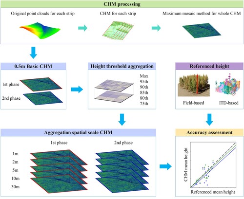
The process diagram of the study is shown in Figure 1. We processed the initial point cloud data to generate CHMs strip by strip, followed by the application of a maximum mosaic method to composite panoramic CHM. The difference in CHMs between two distinct periods served as the basis for detecting variations in canopy height over the four years. Subsequently, field measurement data and individual tree segmentation (ITS) results were leveraged to evaluate the accuracy of CHM-based tree height and height changes.

Figure 1. Flowchart of the data analysis methodology.

2.1. Study area

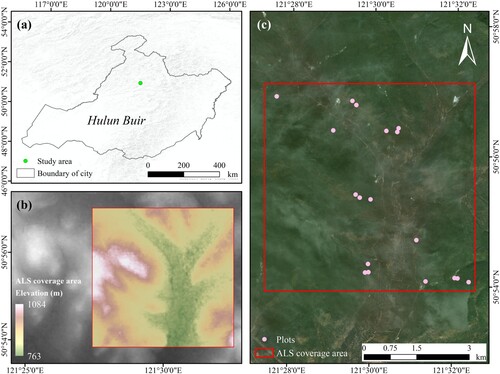
The study area is located in the Genhe forest area in Northeastern China (50° 51′ ∼ 50° 57′ N, 121° 27′ ∼ 121°39′ E). This area is located in the cold temperate continental monsoon climate zone, which exhibits distinct mountainous climatic features. The range of elevation is between 650 and 1269 m. The annual mean precipitation is 450 ∼ 550 mm. And the annual mean temperature is −5.4°C. In terms of whole topography and geomorphology, the river valleys are wide and slight grade with gradients less than 15° comprise over 80% of the region, making the terrain relatively flat (H. Yu and Zhang 2021). The study area has a high forest coverage of approximately 75%, with a complex forest vegetation type and vertical structure. The forest type is mainly coniferous forest. The dominant tree species is Dhurian larch (Larix gmelinii). Other main tree species include white birch (Betula platyphlla) and aspen (populous davidiana) (Huang and Lian 2015).

The natural forest of Greater Khingan Mountains region is an important forest resource industry in China (Yuan et al. 2018). It is also a key forest carbon stock pool in China and highlights its importance in ecological construction strategy and even as an important ecological green barrier for Northeast Asia (W. Gao et al. 2019). Moreover, the Greater Khingan Mountains region is also one of the regions with a high frequency of forest fires in China (F. Guo et al. 2017) (Figure 2).

Figure 2. The study site is located in the Hulun Buir City, Inner Mongolia Autonomous Region, China. The coverage area is indicated by the red frame. It spans a distance of 5700 m from south to north and 5800 m from west to east.

2.2. Data acquisitions

2.2.1. Field plot data

In this research, 17 plots were established in August 2013 and re-measured in August 2016. The field data is from the Dataset of Forest Basic Structural Parameters of the Genhe Experimental Area (Tian et al. 2015). The tree species were Larix gmelinii and Betula platyphylla. Before conducting the experiment, taking into account the characteristics of the complex terrain area combined with high-resolution remote sensing images and digital elevation products, a method of setting up plots based on the south slope, north slope, and different slope was adopted. The investigators of this project were organized to survey the whole experimental area and set up sample plots considering forest type and age. In terms of investigation, square plots were set. The four corners of each plot were positioned by differential global positioning system (DGPS) (GeoXH6000 hand-held receiver and ProXRT base station developed Trimble Inc., USA), and the quadrangle boundaries were measured with a tape. The differential total accuracy was between 0.5 and 0.8 m. The tree height and branch height were measured by laser altimeter (TruPulse® 200 developed by Laser Tech, USA). The crown width (east–west direction and south–north direction) and the relative coordinates of X and Y of the trees in the plot were measured by the tape. The diameter at breast height (DBH) of each tree was measured with a DBH ruler, which all living trees with a DBH greater than 5 cm were measured (Table 1).

Table 1. The airborne laser scanning system parameters.

Species	Plot size (m^2)	number	DBH (cm)	Height (m)
Larix gmelinii	45 × 45	9	8.8 ± 37.7	9.1 ± 37.51
Betula platyphylla	45 × 45	2	10.5 ± 43.0	11.5 ± 22.3
Coniferous mixed forest	45 × 45	3	14.0 ± 43.0	12.6 ± 30.92
Coniferous and broad-leaved mixed forest	45 × 45	3	9.0 ± 31.1	8.15 ± 19.75

Note: x ± y, x is the median of the tree parameters for each tree species, y is the maximum value by which this parameter fluctuates up or down

2.2.2. Airborne remote sensing data acquisitions

Two ALS data were acquired at the same time during August and September in 2012 and 2016 respectively. The datasets consist of LiDAR and CCD data. More detailed devices information in Tables 2 and 3.

Table 2. The airborne laser scanning system parameters.

ALS parameters	Acquisition time
	August 30th, 2012	August 28th, 2016
Aircraft	Yun-5	Yun-5
Flight speed	220 km/h	220 km/h
Flight altitude	2700 m	2200 m
Laser scanning sensor	Leica ALS60	Riegl LMS-Q680i
Wavelength	1064 nm	1550 nm
Laser pulse frequency	200 KHz	200 KHz
Average point density	5.6 pts/m^2	3.2 pts/m^2
Laser beam divergence	0.22 mrad	0.5 mrad
Scan angle	±35°	±30°

Table 3. The airborne CCD system parameters.

CCD parameters	Acquisition time
	August 30th, 2012	August 28th, 2016
CCD sensor	Leica RCD105	IGI DigiCAM-60
Wavelength	RGB	RGB
Resolution	0.5 m	0.5 m
Focal length	60 mm	50 mm
Field of view	55.3°	56.2°
Pixel size	6.8 μm	6 μm

2.3. Methods

2.3.1. ALS data processing

The ALS data from each flight strip was respectively processed using the lidR package for R (Roussel Jean-Romain et al. 2020). First, we preprocessed the ALS data, which includes validating, clipping, noise reduction and ground filtering. Noise removal was performed using statistical outlier removal (SOR) algorithm (Carrilho, Galo, and Santos 2018), while ground and non-ground point classification was carried out using cloth simulation (CSF) algorithm (W. Zhang et al. 2016). The digital terrain model (DTM) was generated using the triangulated irregular network (TIN) algorithm, and the normalized point cloud was obtained by subtracting the pre-processed point cloud from the DTM. Based on the normalized point cloud, the CHM was generated using the Pitfree algorithm (Khosravipour et al. 2014). Both the DTMs and the CHMs were generated with a spatial resolution of 0.5 m. At the same time, the point cloud corresponding to the plots is clipped. We used modified local maximum filter (LMF) algorithm lmfx to detect the tree tops of individual trees and then applying the segmentation algorithm dalponte2016 to depict tree crowns (Dalponte and Coomes 2016; Popescu and Wynne 2004).

2.3.2. CHM generation and mosaic

Strip mosaicking is a crucial step in extracting valuable information from the point cloud of the entire observation area (Blaszczak-Bak, Janicka, and Sobieraj-Zlobinska 2016; Ene et al. 2018). This necessity arises due to factors such as flight altitude, scanning angle of the ALS system, and the narrowness of the swaths (Yongjun Zhang et al. 2015; J. Liu et al. 2018). By mosaicking the ALS point clouds from different flight lines, the density of the point cloud within overlapping areas significantly increases. However, slight discrepancies may exist between adjacent strips, potentially impacting the accuracy of the generated CHM and subsequent estimations of forest parameters (You et al. 2018). Conversely, eliminating duplicate points inadvertently lead to the loss of some valuable information.

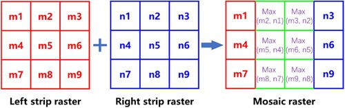
Considering the aforementioned factors, we opted for a methodology capable of generating a seamless CHM. Individual CHMs were first generated for each flight strip, followed by their seamless mosaicking to create a comprehensive CHM, thereby ensuring consistent reference throughout the analysis. Notably, the maximum value mosaicking operation was employed during the mosaicking process. This step is independent of lidR. This maximum mosaic method prioritizes the higher pixel value within the overlapping raster dataset, as illustrated in Figure 3.

Figure 3. Illustration of mosaic operators for maximum. In the overlapping area of the two raster datasets, each pixel is compared between the two rasters to determine the maximum value, which is then used as the value in the resulting mosaic.

2.3.3. Spatial scale aggregation strategy for reveal tree heights

From the normalized point cloud, generating 0.5 m CHMs provides detailed canopy height information and spatial details (Socha et al. 2020). Considering the data coverage and the impact of different scales on canopy height change analysis, we selected five spatial resolutions: 1, 2, 5, 10, and 30 m to evaluate their impact on the estimation of tree height and its change. These resolutions are sufficient to reveal the patterns and relationships of canopy height changes at different scales and time intervals. During the resampling process, we also compared several height metrics, including the maximum value (Hmax), as well as the 75th, 80th, 85th, 90th and 95th percentiles (H75, H80, H85, H90, H95). By combining different resampling scales and height percentile, we subtracted the CHMs from two periods to obtain the difference CHM (ΔCHM) and compared the sensitivity of canopy height differences under different scales and height metrics.

2.3.4. Canopy height variation analysis and accuracy assessment

We extracted the average value of CHMs corresponding to the field plots and compared it with the field-based measurements and ITS-based measurements. Subsequently, the canopy height variation was calculated by subtracting CHM for the 2012 from CHM for the 2016 (Equation (1)). Moreover, we employed analysis of variance (ANOVA) to explore the effects of different height percentile and spatial scales on the accuracy of tree height extracted from the CHM. We evaluated the accuracy of the estimations by using the coefficient of determination (R²), root mean square error (RMSE) and relative RMSE (rRMSE). The values of R², RMSE and rRMSE were calculated as follows: (1) $\begin{array}{c}\mathrm{\Delta }\mathrm{CHM}=\mathrm{CH}{\mathrm{M}}_{2016}-\mathrm{CH}{\mathrm{M}}_{2012}\end{array}$(1) (2) $\begin{array}{c}{R}^2=1-{\displaystyle \frac{{\sum }_{i=1}^n{(y_i-{\hat{y}}_i)}^2}{{\sum }_{i=1}^n{(y_i-\overline{y})}^2}}\end{array}$(2) (3) $\begin{array}{c}\mathrm{RMSE}=\sqrt{{\displaystyle \frac{1}{n}\sum _{i=1}^n{(y_i-{\hat{y}}_i)}^2}}\end{array}$(3) (4) $\begin{array}{c}\mathrm{rRMSE}=\sqrt{{\displaystyle \frac{{\displaystyle \frac{1}{n}{\sum }_{i=1}^n{(y_i-{\hat{y}}_i)}^2}}{{\sum }_{i=1}^n{({\hat{y}}_i)}^2}}}\times 100\text{\%}\end{array}$(4) where: n is the number of field plots, i is the field plots number, $y_i$ is the field-based arithmetic mean height for plot i, ${\hat{y}}_i$ is the predicted height for plot i, $\overline{y}$ is the mean field plot value for all plots.

2.3.5. Assessment of CHM quality

In order to compare and validate the effectiveness of the CHM processing strategy proposed in this paper and its impact on the quality of the CHMs, we also adopted the conventional method to process the data accordingly. The conventional method is to merge all point cloud data together to generate a CHM. The comparison enables an effective assessment of the reliability of proposed method and their impact on the quality of the CHM product.

3. Results

3.1. CHM-based tree height

Figures 4 and 5 illustrated the average tree height estimated from CHM under various spatial scales and height metrics, alongside corresponding values obtained through individual tree segmentation (ITS) and field measurements for the 17 sample plots. From Figure 4, it is evident that as the height percentile increases, there is a gradual increase in the values of R², RMSE, and rRMSE. As can be seen, the fitting accuracy of two phases data exhibit varying performance across different spatial scales and height metrics. 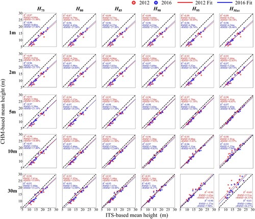According to the statistical assessment metrics, the H90 height percentile with the 5 m spatial scale exhibits the best performance in 2012 ($\mathrm{RMS}{E}_{2012}$ = 2.84 m, $\mathrm{rRMS}{E}_{2012}$ = 22.39%), while 5 m with H85 exhibits the best performance in 2016 ($\mathrm{RMS}{E}_{2016}$ = 2.40 m, $\mathrm{rRMS}{E}_{2016}$ = 17.93%). The most striking observation to emerge from Figure 5 is that the performance of R², RMSE, and rRMSE surpasses that of Figure 4. According to the analysis, it can be observed that 10 m with H95 exhibits the best performance. While the R² value is highest for 5 m with Hmax ($R_{2012}^2$ = 0.98, $R_{2016}^2$ = 0.97), the RMSE and rRMSE values are lowest for 10 m with H95 ($\mathrm{RMS}{E}_{2012}$ = 0.88 m, $\mathrm{rRMS}{E}_{2012}$ = 5.83%, $\mathrm{RMS}{E}_{2016}$ = 1.11 m, $\mathrm{rRMS}{E}_{2016}$ = 6.91%).

Figure 4. Based on different height metrics, comparison of CHM-based and field-based average height estimation results at different resolutions for 2012 and 2016.

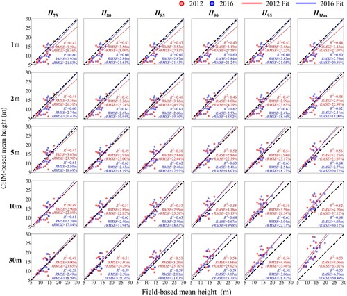
Figure 5. Based on different height metrics, comparison of CHM-based and ITS-based average height estimation results at different resolutions for 2012 and 2016.

3.2. The results of difference CHM variations and accuracy

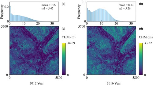
The CHMs, generated with a 0.5 m resolution, revealed significant changes in tree canopy height between 2012 and 2016, as shown in Figure 6. It can also be observed that the average canopy height changed by 1.61 m from 2012 to 2016. The higher proportion of shorter trees and lower canopy in both time periods reflects variations in the vertical structure of the forest within the study area. In 2012, the distribution of canopy height was mainly concentrated in low vegetation, while in 2016, the histogram showed a bimodal distribution. The distribution of canopy heights exhibited a pronounced concentration around 10 meters, indicative of the vertical structure of the forest and the growth dynamics of the vegetation during the period.

Figure 6. (a) and (b) represent the frequency distributions of canopy height for the years 2012 and 2016, respectively. (c) and (d) represent the CHMs for the years 2012 and 2016, respectively.

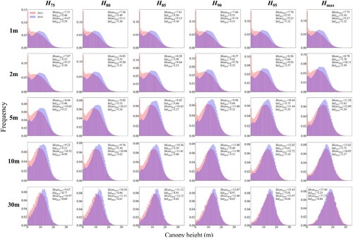
Figure 7 provided an overview of the frequency distribution of canopy heights, including six height percentiles at five resolutions, capturing the canopy vertical structure across two phases. It can be seen from Figure 7 that the standard deviations and average of canopy height for both time periods exhibited a gradually increase with increasing height percentile. It is interesting to note that ultra-low canopy height accounted for a very high proportion in 2012 at the scale of 1–10 m resolution. Additionally, as the scale increased, the shape of crown height frequency distribution approached that of a normal distribution, the proportions of low canopy height more and more less. The overall probability density for 2016 appears to be shifted towards the right compared to 2012, and the peak for 2016 is also higher than that of 2012, indicating forest growth changes.

Figure 7. Based on different height metrics, the frequency distributions of CHMs at different resolutions for the years 2012 and 2016. The red and blue bars represent 2012 and 2016, respectively.

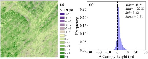
Figure 8 presented the difference between CHM (ΔCHM) and frequency distribution between two periods. It can be observed from Figure 8(a) that there were some fragmentary areas showing negative variations, reflecting noticeable reductions in crown height. However, the majority of areas exhibited increases in canopy height. The results of the statistical analysis are shown in Figure 8(b). It is apparent from average value of 1.61 m that significant growth in canopy height from 2012 to 2016, but standard deviation value shows significant differences in whole study area and there is uneven growth.

Figure 8. (a) Variation in canopy height across the entire study area by two 0.5 m CHMs. (b) The ΔCHM canopy height distribution. The dashed line represents zero value.

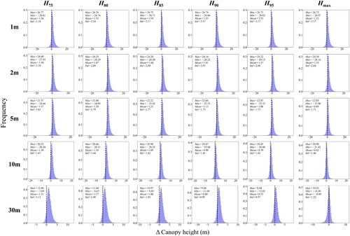
Figure 9 shows the ΔCHM and frequency distribution of six height metrics at five resolutions between two periods. In Figure 9 a clear downward trend can be observed in the average value as the height percentile increases. Conversely, the max, mean and standard deviation show a decreasing trend, while the min shows an increasing trend as the spatial scale increases. From the graph, we can also see that the proportion of negative values increased as the spatial scale increased. The increase in the proportion of negative values was not significant at scales of 1 and 2 m, but it became more noticeable at 10 and 30 m. At the 30 m scale, there was a particularly significant increase in the proportion of negative values. Especially, the proportion of negative values accounts for a half approximately at 30 m with Hmax. Overall, the proportion of positive values was greater than that of negative values.

Figure 9. Histogram of difference canopy height frequency distributions based on six height percentile aggregation at five spatial scale. The dashed lines represent zero values.

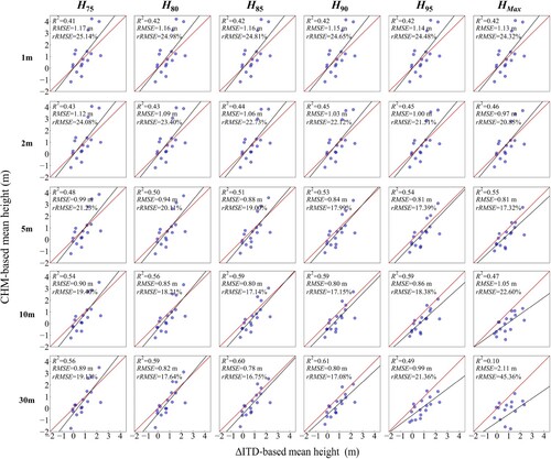
Tables 4 and 5 illustrated the average tree height growth estimated from ΔCHM under various spatial scales and height metrics, alongside corresponding difference values obtained through individual tree segmentation (ITS) and field measurements for the 17 sample plots.

Table 4. Based on different height metrics, comparison of ΔCHM-based and Δfield-based arithmetic mean height estimation results at different resolutions.

Resolution (m)	Assessment Index	Height percentile
		H75	H80	H85	H90	H95	Hmax
1	R^2	0.0025	0.0025	0.0025	0.0024	0.0024	0.0024
	RMSE	1.95	1.94	1.93	1.93	1.92	1.91
	RRMSE	35.07%	34.95%	34.83%	34.71%	34.60%	34.48%
2	R^2	0.0020	0.0019	0.0019	0.0018	0.0017	0.0014
	RMSE	1.90	1.88	1.85	1.83	1.80	1.78
	RRMSE	34.28%	33.82%	33.36%	32.94%	32.50%	31.99%
5	R^2	0.0014	0.0010	0.0009	0.0005	0.0003	0.0007
	RMSE	1.81	1.76	1.71	1.64	1.59	1.54
	RRMSE	32.52%	31.61%	30.72%	29.62%	28.65%	27.74%
10	R^2	0.0003	0.0001	0.0000	0.0000	0.0017	0.0046
	RMSE	1.73	1.67	1.60	1.55	1.50	1.52
	RRMSE	31.11%	30.04%	28.85%	27.96%	27.07%	27.40%
30	R^2	0.0004	0.0024	0.0047	0.0094	0.0076	0.0198
	RMSE	1.70	1.60	1.52	1.44	1.49	2.47
	RRMSE	30.55%	28.83%	27.29%	25.97%	26.83%	44.50%

Table 5. Based on different height metrics, comparison of ΔCHM-based and ΔITS-based arithmetic mean height estimation results at different resolutions.

Resolution (m)	Assessment Index	Height percentile
		H75	H80	H85	H75	H95	max
1	R^2	0.41	0.42	0.42	0.42	0.42	0.42
	RMSE	1.17	1.16	1.16	1.15	1.14	1.13
	RRMSE	25.14%	24.98%	24.81%	24.65%	24.48%	24.32%
2	R^2	0.43	0.43	0.44	0.45	0.45	0.46
	RMSE	1.12	1.09	1.06	1.03	1.00	0.97
	RRMSE	24.08%	23.40%	22.73%	22.12%	21.51%	20.85%
5	R^2	0.48	0.50	0.51	0.53	0.54	0.55
	RMSE	0.99	0.94	0.88	0.84	0.81	0.81
	RRMSE	21.23%	20.11%	19.00%	17.99%	17.39%	17.32%
10	R^2	0.54	0.56	0.59	0.59	0.59	0.47
	RMSE	0.90	0.85	0.80	0.80	0.86	1.05
	RRMSE	19.40%	18.21%	17.14%	17.15%	18.38%	22.60%
30	R^2	0.56	0.59	0.60	0.61	0.49	0.10
	RMSE	0.89	0.82	0.78	0.80	0.99	2.11
	RRMSE	19.13%	17.64%	16.75%	17.08%	21.36%	45.36%

As depicted in Tables 4 and 5, when compared to the results obtained using the difference ITS-based (ΔITS-based) approach, the outcomes derived from the difference field-based (ΔField-based) approach are less satisfactory. Additionally, the most notable observation from Tables 4 and 5 is that the RMSE values are consistently below 2 m, with the exception of 30 m with Hmax. Especially for the ΔITS-based approach, except for 30 m with Hmax, the RMSE values are below 1.2 m, which demonstrates the reliability of using ALS point clouds for direct detection of canopy height variation. According to the statistical assessment metrics, the 30 m with H90 exhibits the best performance in ΔField-based approach (RMSE = 1.44 m, rRMSE = 203.07%), while 30 m with H85 exhibits the best performance in ΔITS-based approach (RMSE = 0.78 m, rRMSE = 91.97%).

3.3. The results of ANOVA

ANOVA was employed to evaluate the impact of height percentile and spatial scale on the CHM. Initially, we conducted one-way ANOVA for each factor to examine their potential effects on the CHM. Subsequently, we performed a two-way ANOVA to determine whether the interaction between two factors significantly influenced the CHM. Table 6 displays the statistical measures, including mean values, of CHM for the sample plots at each resolution and height percentile. Table 7, on the other hand, presents the results of the ANOVA analysis at a significance level of 0.05. The ANOVA results indicate that the calculated F-statistic values for both height percentile and spatial scale are higher than their respective F probability values. The finding suggests that both individual factors and their interaction have a significant effect on the CHM’s characterization of canopy height variation. As shown in Table 6, at height percentiles of H80 and above, the mean values increase by at least 0.5 m as spatial scale increases within the same height percentile. The results emphasized the importance of considering both height percentile and spatial resolution when utilizing dual-time-phase CHM to characterize canopy height change. Selecting the appropriate height percentile and spatial scale is essential for enhancing the accuracy of canopy height change estimation.

Table 6. Statistical parameters of mean values at different resolutions and height percentiles of the CHM raster corresponding to the data from the two sample periods.

Height percentile	Resolution (m)	Number of samples	Mean (m)	Standard deviation (m)	Standard error of mean (m)	Variance (m^2)
H75	1	34	11.10	3.84	0.66	14.71
H75	2	34	11.46	3.87	0.66	14.97
H75	5	34	12.27	4.01	0.69	16.04
H75	10	34	12.91	4.02	0.69	16.12
H75	30	34	13.47	4.04	0.69	16.31
H80	1	34	11.15	3.84	0.66	14.73
H80	2	34	11.63	3.88	0.67	15.08
H80	5	34	12.60	4.02	0.69	16.13
H80	10	34	13.37	4.04	0.69	16.29
H80	30	34	13.95	4.03	0.69	16.25
H85	1	34	11.19	3.84	0.66	14.75
H85	2	34	11.79	3.89	0.67	15.10
H85	5	34	12.96	4.02	0.69	16.18
H85	10	34	13.87	4.06	0.70	16.47
H85	30	34	14.50	4.03	0.69	16.28
H90	1	34	11.24	3.84	0.66	14.78
H90	2	34	11.95	3.89	0.67	15.15
H90	5	34	13.37	4.04	0.69	16.29
H90	10	34	14.44	4.06	0.70	16.48
H90	30	34	15.18	4.07	0.70	16.60
H95	1	34	11.29	3.85	0.66	14.80
H95	2	34	12.13	3.90	0.67	15.23
H95	5	34	13.86	4.05	0.70	16.44
H95	10	34	15.19	4.06	0.70	16.51
H95	30	34	16.16	4.22	0.72	17.81
Hmax	1	34	11.34	3.85	0.66	14.82
Hmax	2	34	12.34	3.91	0.67	15.32
Hmax	5	34	14.58	4.09	0.70	16.77
Hmax	10	34	16.59	4.13	0.71	17.03
Hmax	30	34	19.64	4.88	0.84	23.83

Table 7. ANOVA statistic of the effect of spatial resolution and height percentile on the CHM at the 0.05 significance level.

	ANOVA components	Degree of freedom	Mean square	F statistic	F probability
Height percentile	Model	5	156.41	8.36	0.00
	Error	1014	18.71
	Total	1019
Resolution	Model	4	626.59	36.87	0.00
	Error	1015	16.99
	Total	1019
Two-way	Height percentile	5	156.41	9.71	0.00
	Resolution	4	626.59	38.90	0.00
	Interaction	20	25.95	1.61	0.04
	Model	29	131.29	8.15	0.00
	Error	990	16.11
	Total	1019

3.4. Comparison of ΔCHM consistency between the two strategies

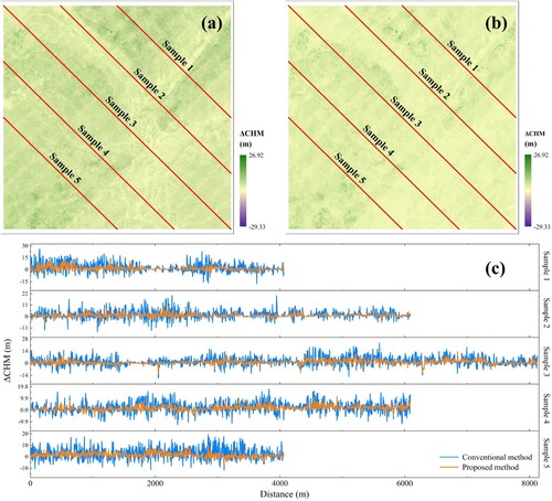
After obtaining CHMs using both the conventional and the proposed methods, we calculated the ΔCHMs. We analyzed the profiles of the ΔCHMs for each of the five selected sampling strips. As shown in Figure 10, there is a significant difference between the two methods of generating CHM. We selected five sampling strips with different length to extract ΔCHM profiles. The proposed method exhibits more stable, while the conventional method shows more drastic.

Figure 10. Five sampling strips comparing the consistency of ΔCHM generated by the two strategies. (a) Conventional method-derived 0.5 m ΔCHM. (b) Proposed method-derived 0.5 m ΔCHM. (c) Comparison of ΔCHM profiles for 5 sampling strips.

4. Discussion

4.1. The impact of point cloud density and height metrics on detecting variations in canopy height

Previous studies had consistently revealed an underestimation of canopy height from LiDAR scanning, point cloud density is one of the most important factors in canopy height underestimation (Fradette et al. 2019; Lefsky et al. 2002). Ideally, researchers hope that the point cloud density is large enough to fully capture the detailed three-dimensional information from the canopy to the ground. However, in scenarios with sparse point cloud density, the inadequate sampling will lead to the omission or scarcity of laser points on the upper portions of canopies. Consequently, canopy height may be underestimated, presenting difficulties in evaluating forest growth patterns. In Hawryło et al. study, they employed low-altitude ALS to detect top height with a density of 597 pts/m² (points per square meter). They discovered that employing ALS data enables a direct measurement of TH at stand-level in this manner (Hawryło et al. 2024). This result illustrates the importance of point cloud density in accurately measuring tree height using ALS data.

Height percentile is highly sensitive to canopy height estimation, which is a variable commonly used in modeling of stand parameters estimation in previous studies (Adnan et al. 2021; Cao et al. 2019). The higher height percentile metrics (such as H95, H99, H100) usually represent the vertical structure extending from the top of the tree and above the canopy. Therefore, the height percentile can provide more information about the growth status and competition of trees (Qu et al. 2018). However, in the general ALS data, insufficient sampling results in missing or fewer laser points in the upper part of the canopy. Higher height percentiles (such as H99, H100) indicate the selection of a small proportion of points located at the highest part of the canopy, which may lead to insufficient sample size, uneven spatial coverage and lack of representativeness. The study primarily focused on forest canopy height change, particularly the upper structure, and the high percentile already represents the canopy height change well. Therefore, we did not further analyze the lower height percentile and its change. It is important to note that the growth of understory plants can also be reflected in the lower percentile. Furthermore, if the point cloud density is low, selecting the lower height percentile may not accurately reflect changes in canopy height.

In summary, by selecting appropriate height percentiles for research, we can obtain results that are representative of canopy changes and have certain statistical significance. Similar to the findings of Socha et al. study, the use of the H99 to measure TH will lead to an underestimation of TH increments in multi-temporal ALS data (Socha et al. 2017; 2020). And in Hawryło et al. study, they also found that if ALS data alone is used without field measurements, the reliable measurement of TH can be achieved through the utilization of either the ITS or the LiDAR-derived Max metric (Hawryło et al. 2024).

We selected a field plot to illustrate this. From the highlighted points in Figure 11(a) and (b), it can be seen that the ITS-based was quite different from the field-based. The highlighted plot illustrates a decrease in canopy height variation based on the ITS-based approach, while the field-based approach demonstrates an increase. Besides, From the highlighted point in Figure 11(c), it can be seen that ITS-derived max height shows a decrease. This variation suggested that the second phase of ALS data did not capture the TH. The plot consists of a mixed forest of Larix gmelinii and Betula platyphylla. Our ground survey data revealed that the tallest tree was a Larix gmelinii within this plot. It is challenging for LiDAR to accurately detect and measure the top height of coniferous trees.

Figure 11. (a) The mean height of field-based in plots in 2012 and 2016. (b) The mean height of ITS-based in plots in 2012 and 2016. (c) The max height of LiDAR-derived in plots in 2012 and 2016. (d) (e) The highlighted plot in (a) (b) (c) corresponds to the CHM in 2012 and 2016. (f) The highlighted plot corresponds to the point cloud in 2012 and 2016, three representative sub-regions were selected in (i) (ii) (iii).

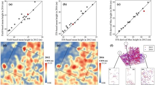
When the same tree shows little growth, the pulses hit the tree at different altitudes during the two observation times. This makes it challenging to determine whether there is real growth or loss (Figure 11 (f)). We refer to this situation as pseudo-growth or pseudo-loss, as it can create a misleading impression of tree growth or decline. Although the LiDAR-derived max height decreased, there was an increase in crown width within indicative of tree growth (Figure 11(d) and (e)).

4.2. Analysis of temporal changes in canopy height

The unique geographical features of the study area make it one of the sensitive areas responsive to global climate change (Q. Zhang et al. 2023). Forest logging is one of the main disturbances in this forest region. Prior to the 1990s, the forested areas in Northeast China experienced long-term logging practices, resulting in significant loss of pristine forests. However, since the 1990s, the government has implemented policies to protect forest ecological resources and imposed restrictions on logging activities in the Northeast China forest region (Yuzhen Zhang and Liang 2014). The Genhe Forest Region ceased all commercial logging activities in April 2015 (Y. Liu et al. 2023). During the period from 2012 to April 2015, there were still small-scale logging operations taking place, resulting in a noticeable reduction in canopy height in localized areas (Figure 12(A)).

Figure 12. Four representative sub-regions to explore the possible factors of canopy height change in the study area. (i) and (ii) are CHM in 2012 and 2016; (iii) and (iv) are CCD images in 2012 and 2016; (v) and (vi) are point cloud height profiles in 2012 and 2016; (vii) is CHM height frequency distribution statistics, the red line and blue line respectively represent 2012 and 2016. (a) indicates the presence of logging; (b) indicates less growth; (c) indicates forest road development; (d) indicates more growth.

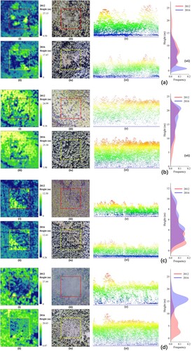
Under the background of implementing the Natural Forest Protection Project, the Greater Khingan Mountains forest region has carried out large-scale artificial afforestation to replace harvested areas with new forests. This includes reforestation efforts on logging sites (Qiu et al. 2020). This conservation project has also facilitated positive changes in forest coverage within the study area (Sun and Tian 2019). In addition to natural tree growth, the management practices in the forest region also have an impact on the variation in canopy height. Larix gmelinii is one of the main dominant tree species in this forest region. However, due to long-term management practices, larch plantations are often managed for fast-growing and high-yield purposes (G. Qi et al. 2013). The average annual growth rate of larch plantations exceeds 0.60 m (Jia et al. 2021), and after reaching canopy closure, the average annual growth can reach around 0.8–1 meter (Mao et al. 2022) (Figure 12(B,D)).

Obvious forest road construction can be seen through CHM and CCD images (Figure 12(C)). In addition to harvesting and policies, human disturbance factors also include forest landscape construction and development. After the full implementation of the natural forest resource protection project and the policy of stopping commercial logging, the region will no longer rely on wood to generate income. The region will be transformed into eco-tourism, and tourism such as parks and scenic spots will be built. Road construction in forest area is mainly for forest fire monitoring and prevention and tourism resources development (Shi et al. 2022).

We identified areas where significant changes in canopy height by comparing bi-temporal CHM. Combining known anthropogenic and natural factors in the area reveals the possible influence of these factors on CHM variation. The findings provide a scientific basis for understanding changes in canopy height, which will help us to better predict and manage future forest changes and improve our understanding of forest ecosystems.

4.3. The impact of aggregation scales on detecting canopy height

At a larger spatial scale, a pixel contains more canopies, understory and ground information. While at smaller spatial scales, more local variations, spatial heterogeneity and significant local height differences can be observed. Figure 9 showed that the frequency distribution of difference canopy height at different resolution, we can obviously see that there is a lot of negative values, especially 10 m with Hmax and 30 m with Hmax. In summary, at the 30 m scale, a significant number of pixels are aggregated. In 2016, due to lower point cloud density, the Max aggregation method did not capture the higher positions of the canopy. This is evident in the ΔCHM, where pixels with negative values indicate that the Max value at the 30 m scale in 2016 is lower than in 2012. When using the Max aggregation method, negative values are also most prevalent when aggregating pixels at other scales. Smaller scales have fewer aggregated pixels and less cumulative error, while larger scales have more aggregated pixels and greater cumulative error. In addition, point cloud density also affects the retrieval of understory vegetation and lower height shrub information. In cases of low point cloud density, insufficient information about lower height vegetation is captured, resulting in negative values after performing the difference operation on the two CHMs.

On the other hand, Figure 7 illustrates that the canopy height frequency distribution of the two periods CHMs at different scales. The larger scales filter out high-frequency variation signals, resulting in the loss or smoothing of surface details, including terrain features and vegetation structural differences. At the same time, this filtering also reduces the impact of noise and outliers. However, such as 30 m scale cannot accurately reflect the canopy height distribution. Hence, the selection of suitable scales and height percentile is crucial for accurately estimating changes in canopy height.

Furthermore, Sharma et al. pointed out that the determination of TH depends on the size of the plot and the number of trees within the plot (Sharma, Amateis, and Burkhart 2002). Figure 4 and Table 4 showed that the results were not good. This discrepancy indicates a large variability between the field-measured data and the CHM, as well as some sampling errors. The average height calculated based on field data is obtained by measuring the tree height of all individual trees within the sample plot and taking the arithmetic mean. Besides, the errors of field measurements from two time periods also contribute to the unreliability of the difference field-based results. For CHM, even at a fine scale like 1 and 2 m, each pixel contains complex information. Some pixels only have canopy, while others mix both canopy and ground. We set the size of the sample plot as 45 × 45 m, at the 30 m, the corresponding CHM for the field plot contains on 1–2 pixels. However, by aggregating the height percentiles and maximum values, we make use of the canopy information as much as possible and avoid interference from ground information. This also indicates the results of Tables 4 and 5, where the 30 m scale aggregate more canopies, thus exhibiting higher accuracy in characterizing canopy height differences than other scales. In Qi et al. study, they mapped the aboveground carbon density variation based on bi-temporal ALS data at 30 m scale (Z. Qi et al. 2023). But in summary, the reliability of characterizing canopy height variation through the 30 m resolution CHM remains insufficient.

From the perspective of inventory, we excluded trees with DBH less than 5 cm during our measurements. Additionally, in some plot surveys and scientific studies, only living trees within the plot are recorded, excluding small DBH trees, dead trees, and fallen trees (Kershaw Jr et al. 2016). However, this also affects the calculation of average canopy height for the plot. The point cloud data in LiDAR scanning are random and can adequately capture the spatial variability within the plot (Z. Qi et al. 2023; Zhao et al. 2018). Nevertheless, the situation is different for tree height estimation. Therefore, in order to accurately describe the canopy height within specific forest environments during field inventory, it is advisable to measure every tree, including those with DBH less than 5 cm. This also shows the advantages of ALS in characterizing forest growth and variation by providing a wide range of continuous data coverage. In our dataset, the individual tree measurements were only recorded once, which has an uncertain effect on the validation of the results. According to the experiment of Persson et al., the contribution of measurement error to the total variance is almost negligible (Persson 2022). Moreover, the investigators involved in the ground measurements were experienced, so it can be assumed that the measurement error had little impact on this study. However, in future experiments, a multiple measurement strategy and new statistical methods should be adopted to take into account the uncertainty of the field measurements in the statistical analyses, especially when validating such analyses of multi-temporal canopy height variations.

On the other hand, we assessed the performance of CHM and ΔCHM at different height percentile and spatial scales using Field-based and ITS-based reference values. As the scale increases, the performance of CHM in estimating canopy height from underestimation to overestimation (Figures 4 and 5), whereas the performance of ΔCHM in estimating canopy height changes from overestimation to underestimation (Tables 4 and 5). In this study area, it is challenging to observe tree tops through field measurements, resulting in underestimation. ITS relies on point cloud information, and inadequate point cloud density leads to underestimation when identifying tree tops from the point cloud. Evaluating canopy height through ITS at a large spatial scale poses computational challenges, consuming significant time and resources. In contrast, CHM can be performed at multiple scales, reducing the ITS complexity. Therefore, overall, CHM is more advantages for assessing canopy height and its changes over multiple temporal periods.

Based on the comprehensive analysis of the results, it seems that 10 m scale is a good choice. In Socha et al. study, they evaluated the effects of different height percentile metrics and grid cell sizes on the trajectory of site index models developed based on bi-temporal ALS data. They found that the grid size did not affect the tree growth trajectory obtained by the model. Regardless of the grid size, the model trajectories obtained by the given TH estimation method are almost the same. In addition, they found that using 50 m grid to estimate stand TH can reduce model fitting residuals. However, 10 m grid can also be applied in remote sensing applications. Calculating TH using 10 m grid can reduce errors caused by local variations in site conditions and average random errors (Socha et al. 2017; 2020).

At the same time, in our results, we also found that the 5 m scale performance was notably satisfactory (Figure 4), with a few metrics even surpassing the 10 m scale. Zhao et al. simply stated the choice of 5 m was due to the trade-off between spatial details and heterogeneity within the grid in their research (Zhao et al. 2018). For our study area, previous studies had also shown similar choice. Gao et al. and Hu et al. also used 5 m resolution for mapping plant area density (PAD) and leaf area index (LAI) in the area (G. Gao et al. 2023; Hu et al. 2018), 5 m scale could effectively represent the variations in canopy height across large forest areas while preserving detailed features. However, they did not explain why they chose 5 m. Our results would provide a reference for canopy height mapping in other similar environments.

4.4. The impacts of stripes overlap on generating CHM

The quality of the ALS-derived CHM is also closely related to strips overlap. Appropriate strip overlap enhances data acquisition efficiency and reduces areas with missing data. For bi-temporal ΔCHM calculation, accurate representation of canopy height variation requires that the two CHMs are accurately co-registered (pixel by pixel aligned) (X. Yu et al. 2006). The purpose is to ensure that the pixels match and the difference operation accurately expresses the canopy height change, however, as shown in Figure 8(a), there are some stripes. The single-phase CHM is normal as shown in Figure 6. However, stripes appeared after the differential calculation.

The generation of striation is attributed to errors existing between flight strips. As a complex system comprising multiple hardware components, such as the aircraft platform, position and orientation system (POS), and laser scanning sensors, the ALS system is susceptible to cumulative errors among its various parts. These inter-component errors result in offsets between corresponding points across different flight strips, consequently compromising the accuracy of the point cloud data. Although the ALS data were acquired on similar dates in the two periods, there are differences due to variations in flight altitude and LiDAR equipment used. Additionally, there are differences between flight paths during both acquisitions, along with some errors between adjacent strips.

In our approach, we accounted for the vertical errors present between flight strips by implementing a strip-wise processing strategy for the point cloud data. Each flight strip’s point clouds were normalized to generate individual CHMs, which were then merged to form an entire CHM. This method effectively reduces the vertical errors between flight strips to some extent. By normalizing within each strip, the data within individual strips are rendered relatively consistent, establishing a common vertical reference frame for the point cloud data of each strip. It facilitates a more straightforward observation of canopy height. After the merging, these deviations are not readily apparent in the single-period CHM. However, as absolute height differences between flight strips persist, these discrepancies are carried over into the combined CHM. Consequently, when calculating the ΔCHM, these variations show as striping artifacts.

In many previous forestry studies of multi-temporal ALS, the process of generating CHM only describes algorithm, but does not describe CHM derived from multiple strips. The general practice is to merge all point clouds to obtain an entire CHM, and also by harmonizing multi-temporal DEM, a relatively reliable DEM is obtained as a benchmark, and the DSM is subtracted from the benchmark DEM to obtain CHM (Cao et al. 2016; Økseter et al. 2015; Riofrio et al. 2022; X. Yu et al. 2004). However, the harmonizing result will also be affected by factors such as point cloud density, side overlap rate, interpolation algorithm and ground point segmentation algorithm.

In practice, it is difficult for the flight platform to achieve consistent or similar flight parameters when obtaining data many times, which affects the quality of multi-temporal ALS data. Fradette et al. proposed a method to reduce the deviation between DEM and CHM based on LiDAR data, which reduced the average deviation from 0.70 to 0.02 m (Fradette et al. 2019). However, the forest environment in different regions is also different, and the transferability of the method is not clear. We adopt the strategy of generating CHM and then splicing by strips, which can reduce the height error between strips to a certain extent, so as to obtain more accurate canopy height information. As depicted in Figure 10, the ΔCHM derived from our proposed method exhibits reduced fluctuation and increased stability in canopy height variations. The result shows the reliability of our approach, which is generating the entire CHM through strip-wise processing of the data.

In summary, errors in flight strips directly affect the reliability and effectiveness of CHMs in applications such as detecting canopy height variations and analyzing forest structure. Therefore, in future research, it is advisable to establish obvious markers on roads and within forested areas as reference objects for point cloud data registration. Additionally, it is essential to evenly distribute ground control points across the terrain to ensure precise processing of ALS data. After fine flight strips matching, the resultant CHM may be a more precise representation of canopy height, and multi-temporal CHMs may be a more accurate demonstration of canopy height variations.

On the other hand, we chose the way to take the maximum value between the overlapping pixels on the CHM grid mosaic. The maximum value composite method is most commonly used to use NDVI to monitor vegetation phenological characteristics. It can eliminate possible anomalies or errors in the data and find out whether the vegetation changes significantly in a specific period of time (Cheng et al. 2023). For land use, for forest areas, among all the divided land use types, maximum synthesis can make forests take precedence over other types (He et al. 2021; Wijedasa et al. 2012). According to the height statistics of Figure 5, most of the height is concentrated between about 5–15 meters. Most of the study area is forest and there are few buildings. Taking the maximum value can ensure the selection of higher object features in the overlapping area, which helps to avoid the problem of local terrain feature loss or blurring caused by data loss or sensor error. And taking the maximum value will give priority to the top height of the canopy measured at a higher position, thereby increasing the ability to observe details and changes in the vertical direction.

Additionally, in overlapping regions between strips, point cloud density increases significantly compared to non-overlapping areas which results in distinct characteristics. These differences can have an impact on extracting forest structural parameters within specific regions. You et al. studied the effects of strips overlap on the estimation of forest structural parameters by ALS data. By comparing and analyzing the average overestimation results of the stands at each height percentile, it was found that the original LiDAR point cloud data had the lowest estimation accuracy, and the separation of overlapping points along the adjacent flight strips could effectively improve the estimation accuracy of the average height of the stands (You et al. 2018). In our study, we did not discuss the advanced processing of point cloud data, such as strip registration, removal of overlapping points, and other associated procedures. Although the presence of overlapping points does exert some influence on the estimation of forest height, we contend that these points actually enhance the characterization of the forest's vertical structure. Moreover, we suggest that regions with high point cloud density and significant overlap warrant closer examination. Future research should focus on refining the processing of point cloud data in these areas to minimize information loss, eliminate redundant points, and decrease the computational expense of data processing.

5. Conclusion

In our research, we proposed a maximum mosaic approach to generate CHM by dividing the flight strips, and then acquire the CHM of the entire study area by taking the maximum value. This method can reduce vertical error between the strips and characterize the forest canopy height more accurately. However, in order to reduce the impact of various factors on point cloud information, it is recommended to use 10 m scale CHM to analyze forest change. For height metrics, although the maximum value can better express the height of the canopy, the point cloud will make the maximum value represent the canopy height inaccurate due to many factors, and it will be more appropriate to select 95th height percentile. ITS-based extraction of canopy height may be a preferable alternative, as it will capture a greater amount of information from the canopy compared to field measurements.

As multi-temporal ALS data is an increasingly common and mature way to acquire data, it is necessary to understand how to better extract robust characteristics to quantify the dynamic information of forests over time. In addition, how to use a simple and efficient point cloud data processing method to characterize canopy changes makes ALS more practical in large-scale forest survey and management.

Disclosure statement

No potential conflict of interest was reported by the author(s).

Correction Statement

This article has been corrected with minor changes. These changes do not impact the academic content of the article.

Additional information

Funding

This work was supported by the National Natural Science Foundation of China (grant numbers 42192580, No.42130111 and No. 42001279).

Appendix

Figure A1. (a) and (b) are the fitted growth curves of Larix gmelinii and Betula platyphylla respectively. We established Schumacher growth functions of Larix gmelinii and Betula platyphylla using the tree age and tree height sampling data from the dataset. Based on the theoretical application of the Schumacher growth function (Burkhart and Tomé 2012).

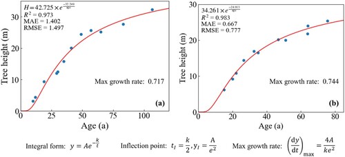
Figure A2. The high resolution figure of Figure 4.

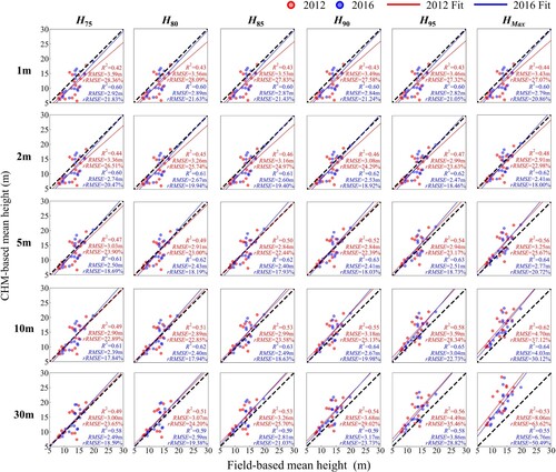
Figure A3. The high resolution figure of Figure 5.

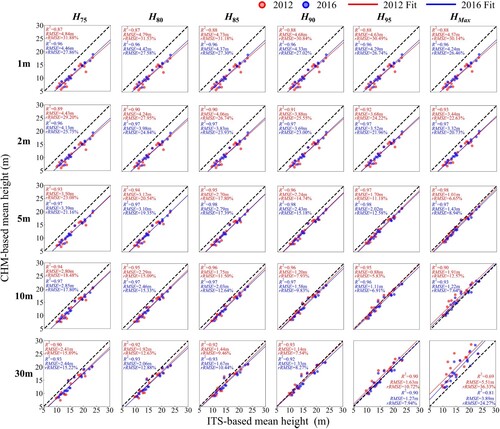
Figure A4. The scatter plot corresponding to Table 4. Based on different height metrics, comparison of ΔCHM-based and Δfield-based arithmetic mean height estimation results at different resolutions.

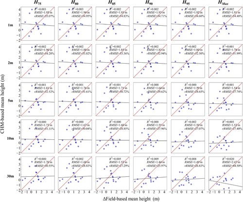
Figure A5. The scatter plot corresponding to Table 5. Based on different height metrics, comparison of ΔCHM-based and ΔITS-based arithmetic mean height estimation results at different resolutions.

References

- Adnan, Syed, Matti Maltamo, Lauri Mehtätalo, Rhei N.L. Ammaturo, Petteri Packalen, and Rubén Valbuena. 2021. “Determining Maximum Entropy in 3D Remote Sensing Height Distributions and Using it to Improve Aboveground Biomass Modelling via Stratification.” Remote Sensing of Environment 260 (July): 112464. https://doi.org/10.1016/j.rse.2021.112464.
- Asokan, Anju, and J. Anitha. 2019. “Change Detection Techniques for Remote Sensing Applications: A Survey.” Earth Science Informatics 12 (2): 143–160. https://doi.org/10.1007/s12145-019-00380-5.
- Beese, Lucy, Michele Dalponte, Gregory P. Asner, David A. Coomes, and Tommaso Jucker. 2022. “Using Repeat Airborne LiDAR to Map the Growth of Individual Oil Palms in Malaysian Borneo During the 2015–16 El Niño.” International Journal of Applied Earth Observation and Geoinformation 115 (December): 103117. https://doi.org/10.1016/j.jag.2022.103117.
- Blaszczak-Bak, Wioleta, Joanna Janicka, and Anna Sobieraj-Zlobinska. 2016. “Applying Ransac Algorithm for Fitting Scanning Strips from Airborne Laser Scanning.” Civil and Environmental Engineering Reports 23 (4): 29–42. https://doi.org/10.1515/ceer-2016-0048.
- Burkhart, Harold E., and Margarida Tomé. 2012. Modeling Forest Trees and Stands. Dordrecht: Springer Netherlands. https://doi.org/10.1007/978-90-481-3170-9
- Cao, Lin, Nicholas C. Coops, John L. Innes, Stephen R.J. Sheppard, Liyong Fu, Honghua Ruan, and Guanghui She. 2016. “Estimation of Forest Biomass Dynamics in Subtropical Forests Using Multi-Temporal Airborne LiDAR Data.” Remote Sensing of Environment 178 (June): 158–171. https://doi.org/10.1016/j.rse.2016.03.012.
- Cao, Lin, Nicholas C. Coops, Yuan Sun, Honghua Ruan, Guibin Wang, Jinsong Dai, and Guanghui She. 2019. “Estimating Canopy Structure and Biomass in Bamboo Forests Using Airborne LiDAR Data.” ISPRS Journal of Photogrammetry and Remote Sensing 148 (February): 114–129. https://doi.org/10.1016/j.isprsjprs.2018.12.006.
- Carrilho, A. C., M. Galo, and R. C. Santos. 2018. “Statistical Outlier Detection Method for Airborne Lidar Data.” The International Archives of the Photogrammetry, Remote Sensing and Spatial Information Sciences XLII–1 (September): 87–92. https://doi.org/10.5194/isprs-archives-XLII-1-87-2018.
- Cheng, Kai, Yanjun Su, Hongcan Guan, Shengli Tao, Yu Ren, Tianyu Hu, Keping Ma, Yanhong Tang, and Qinghua Guo. 2023. “Mapping China’s Planted Forests Using High Resolution Imagery and Massive Amounts of Crowdsourced Samples.” ISPRS Journal of Photogrammetry and Remote Sensing 196: 356–371. https://doi.org/10.1016/j.isprsjprs.2023.01.005.
- Coops, Nicholas C. 2015. “Characterizing Forest Growth and Productivity Using Remotely Sensed Data.” Current Forestry Reports 1 (3): 195–205. https://doi.org/10.1007/s40725-015-0020-x.
- Dalponte, Michele, and David A. Coomes. 2016. “Tree-Centric Mapping of Forest Carbon Density from Airborne Laser Scanning and Hyperspectral Data.” Methods in Ecology and Evolution 7 (10): 1236–1245. https://doi.org/10.1111/2041-210X.12575.
- Dalponte, Michele, Tommaso Jucker, Sicong Liu, Lorenzo Frizzera, and Damiano Gianelle. 2019. “Characterizing Forest Carbon Dynamics Using Multi-Temporal Lidar Data.” Remote Sensing of Environment 224: 412–420. https://doi.org/10.1016/j.rse.2019.02.018.
- Dong, Pinliang, and Qi Chen. 2017. LiDAR Remote Sensing and Applications. Boca Raton: CRC Press. https://doi.org/10.4324/9781351233354
- Ene, Liviu T., Terje Gobakken, Hans-Erik Andersen, Erik Næsset, Bruce D. Cook, Douglas C. Morton, Chad Babcock, and Ross Nelson. 2018. “Large-Area Hybrid Estimation of Aboveground Biomass in Interior Alaska Using Airborne Laser Scanning Data.” Remote Sensing of Environment 204 (January): 741–755. https://doi.org/10.1016/j.rse.2017.09.027.
- Fradette, Marie-Soleil, Antoine Leboeuf, Martin Riopel, and Jean Bégin. 2019. “Method to Reduce the Bias on Digital Terrain Model and Canopy Height Model from LiDAR Data.” Remote Sensing 11 (7): 863. https://doi.org/10.3390/rs11070863.
- Gao, Ge, Jianbo Qi, Simei Lin, Ronghai Hu, and Huaguo Huang. 2023. “Estimating Plant Area Density of Individual Trees from Discrete Airborne Laser Scanning Data Using Intensity Information and Path Length Distribution.” International Journal of Applied Earth Observation and Geoinformation 118 (April): 103281. https://doi.org/10.1016/j.jag.2023.103281.
- Gao, Weifeng, Yunlong Yao, Hong Liang, Liquan Song, Houcai Sheng, Tijiu Cai, and Dawen Gao. 2019. “Emissions of Nitrous Oxide from Continuous Permafrost Region in the Daxing’an Mountains, Northeast China.” Atmospheric Environment 198: 34–45. https://doi.org/10.1016/j.atmosenv.2018.10.045.
- Guerra-Hernández, Juan, Adrian Pascual, Frederico Tupinambá-Simões, Sergio Godinho, Brigite Botequim, Alfonso Jurado-Varela, and Vicente Sandoval-Altelarrea. 2024. “Using Bi-Temporal ALS and NFI-Based Time-Series Data to Account for Large-Scale Aboveground Carbon Dynamics: The Showcase of Mediterranean Forests.” European Journal of Remote Sensing 57 (1): 2315413. https://doi.org/10.1080/22797254.2024.2315413.
- Guo, Qinghua, Yanjun Su, and Tianyu Hu. 2023. LiDAR Principles, Processing and Applications in Forest Ecology. 1st ed. Amsterdam, Netherlands: Academic Press.
- Guo, Futao, Zhangwen Su, Guangyu Wang, Long Sun, Mulualem Tigabu, Xiajie Yang, and Haiqing Hu. 2017. “Understanding Fire Drivers and Relative Impacts in Different Chinese Forest Ecosystems.” Science of The Total Environment 605-606: 411–425. https://doi.org/10.1016/j.scitotenv.2017.06.219.
- Hawryło, Paweł, Jarosław Socha, Piotr Wężyk, Wojciech Ochał, Wojciech Krawczyk, Jakub Miszczyszyn, and Luiza Tymińska-Czabańska. 2024. “How to Adequately Determine the Top Height of Forest Stands Based on Airborne Laser Scanning Point Clouds?” Forest Ecology and Management 551 (January): 121528. https://doi.org/10.1016/j.foreco.2023.121528.
- He, Shan, Huaiyong Shao, Wei Xian, Shuhui Zhang, Jialong Zhong, and Jiaguo Qi. 2021. “Extraction of Abandoned Land in Hilly Areas Based on the Spatio-Temporal Fusion of Multi-Source Remote Sensing Images.” Remote Sensing 13 (19): 3956. https://doi.org/10.3390/rs13193956.
- Hu, Ronghai, Guangjian Yan, Francoise Nerry, Yunshu Liu, Yumeng Jiang, Shuren Wang, Yiming Chen, Xihan Mu, Wuming Zhang, and Donghui Xie. 2018. “Using Airborne Laser Scanner and Path Length Distribution Model to Quantify Clumping Effect and Estimate Leaf Area Index.” IEEE Transactions on Geoscience and Remote Sensing 56 (6): 3196–3209. https://doi.org/10.1109/TGRS.2018.2794504.
- Huang, HuaGuo, and Jun Lian. 2015. “A 3D Approach to Reconstruct Continuous Optical Images Using Lidar and MODIS.” Forest Ecosystems 2 (1): 20. https://doi.org/10.1186/s40663-015-0044-5.
- Jean-Romain, Roussel, Auty David, Coops Nicholas, Tompalski Piotr, Goodbody R. H. Tristan, Meador Andrew Sanchez, Bourdon Jean-Francois, de Boissieu Florian, and Achim Alexis. 2020. “lidR: An R Package for Analysis of Airborne Laser Scanning (ALS) Data.” Remote Sensing of Environment 251: 112061. https://doi.org/10.1016/j.rse.2020.112061.
- Jia, Bingrui, Hongru Sun, Herman Henry Shugart, Zhenzhu Xu, Peng Zhang, and Guangsheng Zhou. 2021. “Growth Variations of Dahurian Larch Plantations Across Northeast China: Understanding the Effects of Temperature and Precipitation.” Journal of Environmental Management 292 (August): 112739. https://doi.org/10.1016/j.jenvman.2021.112739.
- Kershaw Jr, John A, Mark J. Ducey, Thomas W. Beers, and Bertram Husch. 2016. Forest Mensuration. 5th ed. Chichester ; Hoboken, NJ: Wiley-Blackwell.
- Khosravipour, Anahita, Andrew K. Skidmore, Martin Isenburg, Tiejun Wang, and Yousif A. Hussin. 2014. “Generating Pit-Free Canopy Height Models from Airborne Lidar.” Photogrammetric Engineering & Remote Sensing 80 (9): 863–872. https://doi.org/10.14358/PERS.80.9.863.
- Lang, Nico, Walter Jetz, Konrad Schindler, and Jan Dirk Wegner. 2023. “A High-Resolution Canopy Height Model of the Earth.” Nature Ecology & Evolution 7 (11): 1778–1789. https://doi.org/10.1038/s41559-023-02206-6.
- Lefsky, Michael A., Warren B. Cohen, Geoffrey G. Parker, and David J. Harding. 2002. “Lidar Remote Sensing for Ecosystem Studies.” Bioscience 52 (1): 19. https://doi.org/10.1641/0006-3568(2002)052[0019:LRSFES]2.0.CO;2.
- Li, Chenyun, Zhexiu Yu, Shaojie Wang, Fayun Wu, Kunjian Wen, Jianbo Qi, and Huaguo Huang. 2022. “Crown Structure Metrics to Generalize Aboveground Biomass Estimation Model Using Airborne Laser Scanning Data in National Park of Hainan Tropical Rainforest, China.” Forests 13 (7): 1142. https://doi.org/10.3390/f13071142.
- Liu, Qianwei, Weifeng Ma, Jianpeng Zhang, Yicheng Liu, Dongfan Xu, and Jinliang Wang. 2021. “Point-Cloud Segmentation of Individual Trees in Complex Natural Forest Scenes Based on a Trunk-Growth Method.” Journal of Forestry Research 32 (6): 2403–2414. https://doi.org/10.1007/s11676-021-01303-1.
- Liu, Jing, Andrew K. Skidmore, Simon Jones, Tiejun Wang, Marco Heurich, Xi Zhu, and Yifang Shi. 2018. “Large Off-Nadir Scan Angle of Airborne LiDAR Can Severely Affect the Estimates of Forest Structure Metrics.” ISPRS Journal of Photogrammetry and Remote Sensing 136 (February): 13–25. https://doi.org/10.1016/j.isprsjprs.2017.12.004.
- Liu, Yang, Ralph Trancoso, Qin Ma, Philippe Ciais, Lidiane P. Gouvêa, Chaofang Yue, Jorge Assis, and Juan A. Blanco. 2023. “Carbon Density in Boreal Forests Responds Non-Linearly to Temperature: An Example from the Greater Khingan Mountains, Northeast China.” Agricultural and Forest Meteorology 338 (July): 109519. https://doi.org/10.1016/j.agrformet.2023.109519.
- Mao, Chunyan, Lubei Yi, Wenqiang Xu, Li Dai, Anming Bao, Zhengyu Wang, and Xueting Zheng. 2022. “Study on Biomass Models of Artificial Young Forest in the Northwestern Alpine Region of China.” Forests 13 (11): 1828. https://doi.org/10.3390/f13111828.
- Matti, Maltamo, Næsset Erik, and Vauhkonen Jari, Eds. 2014. Forestry Applications of Airborne Laser Scanning: Concepts and Case Studies. Vol. 27. Managing Forest Ecosystems. Dordrecht: Springer Netherlands. https://doi.org/10.1007/978-94-017-8663-8
- Michałowska, Maja, and Jacek Rapiński. 2021. “A Review of Tree Species Classification Based on Airborne LiDAR Data and Applied Classifiers.” Remote Sensing 13 (3): 353. https://doi.org/10.3390/rs13030353.
- Ncutirakiza, Ndamiyehe, Sylvie Gourlet-Fleury Jean-Baptiste, Philippe Lejeune, Xavier Bry, and Catherine Trottier. 2024. “Using High-Resolution Images to Analyze the Importance of Crown Size and Competition for the Growth of Tropical Trees.” Forest Ecology and Management 552 (January): 121553. https://doi.org/10.1016/j.foreco.2023.121553.
- Ochal, W., J. Socha, and M. Pierzchalski. 2017. “The Effect of the Calculation Method, Plot Size, and Stand Density on the Accuracy of Top Height Estimation in Norway Spruce Stands.” iForest - Biogeosciences and Forestry 10 (2): 498–505. https://doi.org/10.3832/ifor2108-010.
- Økseter, Roar, Ole Martin Bollandsås, Terje Gobakken, and Erik Næsset. 2015. “Modeling and Predicting Aboveground Biomass Change in Young Forest Using Multi-Temporal Airborne Laser Scanner Data.” Scandinavian Journal of Forest Research 30 (5): 458–469. https://doi.org/10.1080/02827581.2015.1024733.
- Pang, Yong, Weiwei Wang, Liming Du, Zhongjun Zhang, Xiaojun Liang, Yongning Li, and Zuyuan Wang. 2021. “Nyström-Based Spectral Clustering Using Airborne LiDAR Point Cloud Data for Individual Tree Segmentation.” International Journal of Digital Earth 14 (10): 1452–1476. https://doi.org/10.1080/17538947.2021.1943018.
- Persson, Henrik Jan. 2022. “Quantify and Account for Field Reference Errors in Forest Remote Sensing Studies.” Remote Sensing of Environment 283 (December): 113302. https://doi.org/10.1016/j.rse.2022.113302.
- Popescu, Sorin C., and Randolph H. Wynne. 2004. “Seeing the Trees in the Forest.” Photogrammetric Engineering & Remote Sensing 70 (5): 589–604. https://doi.org/10.14358/PERS.70.5.589.
- Qi, Zhiyong, Shiming Li, Yong Pang, Guang Zheng, Dan Kong, and Zengyuan Li. 2023. “Assessing Spatiotemporal Variations of Forest Carbon Density Using Bi-Temporal Discrete Aerial Laser Scanning Data in Chinese Boreal Forests.” Forest Ecosystems 10: 100135. https://doi.org/10.1016/j.fecs.2023.100135.
- Qi, Guang, Qingli Wang, Xinchuang Wang, Dapao Yu, Li Zhou, Wangming Zhou, Shunlei Peng, and Limin Dai. 2013. “Soil Organic Carbon Storage in Different Aged Larix Gmelinii Plantations in Great Xing’ an Mountains of Northeast China.” The Journal of Applied Ecology 24 (1): 10–16.
- Qiu, Zixuan, Zhongke Feng, Yanni Song, Menglu Li, and Panpan Zhang. 2020. “Carbon Sequestration Potential of Forest Vegetation in China from 2003 to 2050: Predicting Forest Vegetation Growth Based on Climate and the Environment.” Journal of Cleaner Production 252 (April): 119715. https://doi.org/10.1016/j.jclepro.2019.119715.
- Qu, Yonghua, Shaker Ahmed, Silva Carlos, Klauberg Carine, and Pinagé Ekena. 2018. “Remote Sensing of Leaf Area Index from LiDAR Height Percentile Metrics and Comparison with MODIS Product in a Selectively Logged Tropical Forest Area in Eastern Amazonia.” Remote Sensing 10 (6): 970. https://doi.org/10.3390/rs10060970.
- Riofrio, Jose, Joanne C. White, Piotr Tompalski, Nicholas C. Coops, and Michael A. Wulder. 2022. “Harmonizing Multi-Temporal Airborne Laser Scanning Point Clouds to Derive Periodic Annual Height Increments in Temperate Mixedwood Forests.” Canadian Journal of Forest Research 52 (10): 1334–1352. https://doi.org/10.1139/cjfr-2022-0055.
- Sharma, Mahadev, Ralph L. Amateis, and Harold E. Burkhart. 2002. “Top Height Definition and Its Effect on Site Index Determination in Thinned and Unthinned Loblolly Pine Plantations.” Forest Ecology and Management 168 (1-3): 163–175. https://doi.org/10.1016/S0378-1127(01)00737-X.
- Shi, Fang, Mingxing Liu, Jie Qiu, Yali Zhang, Huiyi Su, Xupeng Mao, Xin Li, et al. 2022. “Assessing Land Cover and Ecological Quality Changes in the Forest-Steppe Ecotone of the Greater Khingan Mountains, Northeast China, from Landsat and MODIS Observations from 2000 to 2018.” Remote Sensing 14 (3): 725. https://doi.org/10.3390/rs14030725.
- Socha, Jarosław, Paweł Hawryło, Krzysztof Stereńczak, Stanisław Miścicki, Luiza Tymińska-Czabańska, Wojciech Młocek, and Piotr Gruba. 2020. “Assessing the Sensitivity of Site Index Models Developed Using Bi-Temporal Airborne Laser Scanning Data to Different Top Height Estimates and Grid Cell Sizes.” International Journal of Applied Earth Observation and Geoinformation 91 (September): 102129. https://doi.org/10.1016/j.jag.2020.102129.
- Socha, Jarosław, Marcin Pierzchalski, Radomir Bałazy, and Mariusz Ciesielski. 2017. “Modelling Top Height Growth and Site Index Using Repeated Laser Scanning Data.” Forest Ecology and Management 406 (December): 307–317. https://doi.org/10.1016/j.foreco.2017.09.039.
- Sun, Hong, and Xin Tian. 2019. “Analysis of Dynamic Changes of Fractional Vegetation Coverage and Influencing Factors of the Genhe in the Great Khingan of Inner Mongolia.” Remote Sensing Technology and Application 33 (6): 1159–1169. https://doi.org/10.11873/j.issn.1004-0323.2018.6.1159.
- Tian, Xin, Zengyuan Li, Erxue Chen, Qinhuo Liu, Guangjian Yan, Jindi Wang, Zheng Niu, et al. 2015. “The Complicate Observations and Multi-Parameter Land Information Constructions on Allied Telemetry Experiment (COMPLICATE).” PLoS One 10 (9): e0137545. https://doi.org/10.1371/journal.pone.0137545.
- Tolan, Jamie, Hung-I Yang, Benjamin Nosarzewski, Guillaume Couairon, Huy V. Vo, John Brandt, Justine Spore, et al. 2024. “Very High Resolution Canopy Height Maps from RGB Imagery Using Self-Supervised Vision Transformer and Convolutional Decoder Trained on Aerial Lidar.” Remote Sensing of Environment 300 (January): 113888. https://doi.org/10.1016/j.rse.2023.113888.
- White Joanne, C., Coops Nicholas, Wulder A Michael, Vastaranta Mikko, Hilker Thomas, and Tompalski Piotr. 2016. “Remote Sensing Technologies for Enhancing Forest Inventories: A Review.” Canadian Journal of Remote Sensing 42 (5): 619–641. https://doi.org/10.1080/07038992.2016.1207484.
- Wijedasa, Lahiru S., Sean Sloan, Dimitrios G. Michelakis, and Gopalasamy R. Clements. 2012. “Overcoming Limitations with Landsat Imagery for Mapping of Peat Swamp Forests in Sundaland.” Remote Sensing 4 (9): 2595–2618. https://doi.org/10.3390/rs4092595.
- You, Haotian, Yanqiu Xing, Tao Peng, and Jianhua Ding. 2018. “Research on the Effect of Side-Overlap Between Airborne LiDAR Adjacent Swaths on the Coniferous Forest Structural Parameters Estimation.” SCIENTIA SILVAE SINICAE 54 (6): 109–118. https://doi.org/10.11707/j.1001-7488.20180613.
- Yu, Xiaowei, Juha Hyyppä, Markus Holopainen, and Mikko Vastaranta. 2010. “Comparison of Area-Based and Individual Tree-Based Methods for Predicting Plot-Level Forest Attributes.” Remote Sensing 2 (6): 1481–1495. https://doi.org/10.3390/rs2061481.
- Yu, Xiaowei, Juha Hyyppä, Harri Kaartinen, and Matti Maltamo. 2004. “Automatic Detection of Harvested Trees and Determination of Forest Growth Using Airborne Laser Scanning.” Remote Sensing of Environment 90 (4): 451–462. https://doi.org/10.1016/j.rse.2004.02.001.
- Yu, Xiaowei, Juha Hyyppä, Antero Kukko, Matti Maltamo, and Harri Kaartinen. 2006. “Change Detection Techniques for Canopy Height Growth Measurements Using Airborne Laser Scanner Data.” Photogrammetric Engineering & Remote Sensing 72 (12): 1339–1348. https://doi.org/10.14358/PERS.72.12.1339.
- Yu, Haoyang, and Zhongjun Zhang. 2021. “The Performance of Relative Height Metrics for Estimation of Forest Above-Ground Biomass Using L- and X-Bands TomoSAR Data.” IEEE Journal of Selected Topics in Applied Earth Observations and Remote Sensing 14: 1857–1871. https://doi.org/10.1109/JSTARS.2021.3051081.
- Yuan, Shusheng, Tongtong Tang, Minchao Wang, Hao Chen, Aihua Zhang, and Jinghua Yu. 2018. “Regional Scale Determinants of Nutrient Content of Soil in a Cold-Temperate Forest.” Forests 9 (4): 177. https://doi.org/10.3390/f9040177.
- Zhang, Qiyue, Saeid Homayouni, Pengwu Zhao, and Mei Zhou. 2023. “Burned Vegetation Recovery Trajectory and Its Driving Factors Using Satellite Remote-Sensing Datasets in the Great Xing’an Forest Region of Inner Mongolia.” International Journal of Wildland Fire 32 (2): 244–261. https://doi.org/10.1071/WF21167.
- Zhang, Yuzhen, and Shunlin Liang. 2014. “Changes in Forest Biomass and Linkage to Climate and Forest Disturbances Over Northeastern China.” Global Change Biology 20 (8): 2596–2606. https://doi.org/10.1111/gcb.12588.
- Zhang, Yupan, Yuichi Onda, Hiroaki Kato, Bin Feng, and Takashi Gomi. 2022. “Understory Biomass Measurement in a Dense Plantation Forest Based on Drone-SfM Data by a Manual Low-Flying Drone Under the Canopy.” Journal of Environmental Management 312 (June): 114862. https://doi.org/10.1016/j.jenvman.2022.114862.
- Zhang, Wuming, Jianbo Qi, Peng Wan, Hongtao Wang, Donghui Xie, Xiaoyan Wang, and Guangjian Yan. 2016. “An Easy-to-Use Airborne LiDAR Data Filtering Method Based on Cloth Simulation.” Remote Sensing 8 (6): 501. https://doi.org/10.3390/rs8060501.
- Zhang, Yongjun, Xiaodong Xiong, Maoteng Zheng, and Xu Huang. 2015. “LiDAR Strip Adjustment Using Multifeatures Matched With Aerial Images.” IEEE Transactions on Geoscience and Remote Sensing 53 (2): 976–987. https://doi.org/10.1109/TGRS.2014.2331234.
- Zhao, Kaiguang, Juan C. Suarez, Mariano Garcia, Tongxi Hu, Cheng Wang, and Alexis Londo. 2018. “Utility of Multitemporal Lidar for Forest and Carbon Monitoring: Tree Growth, Biomass Dynamics, and Carbon Flux.” Remote Sensing of Environment 204 (January): 883–897. https://doi.org/10.1016/j.rse.2017.09.007.
- Zhou, Hang, Junxiong Zhang, Luzhen Ge, Xiaowei Yu, Yonglin Wang, and Chunlong Zhang. 2021. “Research on Volume Prediction of Single Tree Canopy Based on Three-Dimensional (3D) LiDAR and Clustering Segmentation.” International Journal of Remote Sensing 42 (2): 738–755. https://doi.org/10.1080/01431161.2020.1811917.