How well do the volunteers label land cover types in manual interpretation of remote sensing imagery?

ABSTRACT

High-quality samples for training and validation are crucial for land cover classification, especially in some complex scenarios. The reliability, representativeness, and generalizability of the sample set are important for further researches. However, manual interpretation is subjective and prone to errors. Therefore, this study investigated the following questions: (1) How much difference is there in the interpreters’ performance across educational levels? (2) Do the accuracies of human and AI (Artificial Intelligence) improve with increased training and supporting material? (3) How sensitive are the accuracies of land cover types to different supporting material? (4) Does interpretation accuracy change with interpreters’ consistency? The experiment involved 50 interpreters completing five cycles of manual image interpretation. Higher educational background interpreters showed better performance: accuracies pre-training at 52.22% and 58.61%, post-training at 61.13% and 70.21%. Accuracy generally increased with more supporting material. Ultra-high-resolution images and background knowledge contributed the most to accuracy improvement, while the time series of normalized difference vegetation index (NDVI) contributed the least. Group consistency was a reliable indicator of volunteer sample reliability. In the case of limited samples, AI was not as good as manual interpretation. To ensure quality in samples through manual interpretation, we recommend inviting educated volunteers, providing training, preparing effective support material, and filtering based on group consistency.

KEYWORDS:

• Image interpretation
• Land cover
• Training and test sample
• Reference material
• Crowdsourcing

1. Introduction

Land cover and land use maps serve as the foundation for monitoring the condition of the Earth's surface and reflecting socio-economic functions. They play a crucial role in various planning and management activities (Das et al. 2021; Hussain et al. 2023; Seyam, Haque, and Rahman 2023; Zhang et al. 2018). However, obtaining high-quality samples is essential for accurate supervised land cover classification. Supervised classifiers typically require high-quality training datasets to achieve optimal classification performance (Maxwell, Warner, and Fang 2018). Traditionally, land cover sample datasets are typically collected through fieldwork (Latifovic, Pouliot, and Olthof 2017; Xu et al. 2023; Zhao et al. 2018), manual interpretation of high-resolution satellite imagery (Latifovic, Pouliot, and Olthof 2017), pre-existing datasets, or land cover maps (Zhao et al. 2016). These methods of collecting samples are very time-consuming and labor-intensive. But now, an exciting new approach is changing the way we collect data, thanks to the power of crowdsourcing. A team of enthusiastic volunteers equipped with GPS devices and or online visualization platforms all contributed to the collection of land cover information (Foody et al. 2022; Fraisl et al. 2022; Tavra, Racetin, and Peroš 2021; Zhao et al. 2017). Whereas, each method of sample collection has its disadvantages: (1) collecting samples through field surveys is the most resource-consuming; (2) samples collected from existing land cover maps may introduce errors; (3) the reliability of volunteer geographic data is difficult to ensure; and (4) it is challenging to standardize and streamline the storage, management, distribution, and utilization of data. To overcome these challenges, a popular approach is the interpretation of high-resolution satellite images by experienced analysts or trained volunteers, which has proven to be effective for sample collection and land cover assessment (Lesiv et al. 2018; Li et al. 2021; Roy et al. 2021; Schepaschenko et al. 2019). To keep volunteers engaged in long-term interpretation, a gamification element has been introduced, making the process enjoyable and rewarding (Watkinson, Huck, and Harris 2023). Meanwhile, the collection of accurate reference samples has been emphasized by researchers, ensuring the reliability of the data (McRoberts et al. 2018). It is necessary to (1) evaluate the consistency of interpreters and the errors in interpretation, (2) analyse the factors affecting the performance of interpreters, and (3) provide sufficient training and reference material to enhance the interpretation performance of image interpreters and minimize errors.

With the rapid development of remote sensing technology and AI, AI interpretation has become an indispensable tool for processing and analyzing remote sensing data. Common methods for AI interpretation include supervised (Cengiz et al. 2023; Tariq et al. 2023) and unsupervised approaches (Bah, Hafiane, and Canals 2023; Kim, Kanezaki, and Tanaka 2020). Supervised methods rely on labeled data to enhance accuracy but require extensive manual labeling (Dimitrovski et al. 2023; Papoutsis et al. 2023; Sadeghi et al. 2023). Although deep learning performs well in supervised learning, it relies on large-scale labeled data and is constrained by opacity and non-interpretability(Sadeghi et al. 2023). Unsupervised methods are suitable for unlabeled data but have limited applicability in high-resolution images (Bah, Hafiane, and Canals 2023). Additionally, geographic knowledge graphs provide interpretable AI perspectives and formalizable descriptions of geographic knowledge, driving intelligence in remote sensing interpretation (Li et al. 2023; Liu et al. 2023). They are mainly categorized into two methods: active guidance and participatory understanding, which help improve interpretation efficiency and accuracy but face challenges related to data quality, maintenance, integration, and interpretability (Janowicz et al. 2020; Krabina 2023). Consequently, machine interpretation algorithms encounter key issues in remote sensing image processing. Firstly, these algorithms typically require a substantial amount of interpreted data for training to accurately identify and interpret specific targets or features in remote sensing images (Wang et al. 2023; Zhang et al. 2023). However, acquiring and interpreting this data rely on manual interpretation. Secondly, AI interpretation is subject to errors and uncertainties, which were caused by algorithm limitations, data quality issues, or insufficient training data, and need to be verified and confirmed with manual interpretation samples (Bai et al. 2023; Raja et al. 2023). Furthermore, there have been limitations to AI interpretation when interpreting complex scenes. In these scenes, there were multiple overlapping, similar, or confusable features, such as urban areas or densely vegetated regions, making it difficult for algorithms to accurately distinguish and identify them (Jiao et al. 2023). In conclusion, the primary constraint of AI interpretation lies in using manual interpretation samples as input for the model. Compared to AI interpretation, manual interpretation has the advantage of strong flexibility. The human visual system has rich perceptual abilities and a wealth of domain reference material, enabling it to identify subtle features and complex relationships among features in remote-sensing images. It was capable of adjusting and making judgments based on specific situations and can interpret the information by combining experience and professional knowledge, especially when presented with visual cues. It possesses a high level of flexibility. Therefore, although AI interpretation has the advantages of efficiency, speed, and repeatability, it still relies on the assistance of manual interpretation samples.

The accuracy of manual interpretation samples is increasingly under scrutiny, as precision relies on the interpreter's personal skills, reference material, and training. Due to variations in education, inconsistent results among different interpreters are common (Kraff, Wurm, and Taubenbck 2020). The experience and professional knowledge of the interpreter significantly impact the accuracy and reliability of manual interpretation. Skilled remote sensing experts can accurately identify and interpret geographical features in images, making judgments and inferences based on their professional knowledge (Tarko et al. 2021). Studies showed that novice interpreters have lower accuracy compared to professional interpreters, indicating the need for interpreter training (Waldner et al. 2019). Lesiv emphasized the importance of having access to images for monitoring changes in cropland using manual interpretation (Lesiv et al. 2018). During the interpretation process, the accuracy of the interpretation may be affected by using different interpretation reference material. Interpretation reference material includes the quality of images and the characteristics of the ground objects themselves. Image quality, including resolution, noise, and the degree of cloud cover, directly affects the accuracy and reliability of manual interpretation. The diversity and complexity of ground features will affect the difficulty and accuracy of manual interpretation. Different surface features exhibit distinct spectral reflection and spatial distribution characteristics, requiring interpreters to possess the ability to comprehend and discern these traits. Mutual occlusion of ground objects will also increase the difficulty of interpretation. This required interpreters to utilize other sources of information, such as multi-temporal images or ground survey data, to address the issue. In addition, the presence of land cover types that are morphologically similar in terms of land use and coverage may be the primary cause of confusion (Waldner et al. 2019). Cropland is a type of land cover that is typically challenging to map, resulting in high uncertainty in global cultivated land maps (AbdelRahman 2023). Domain-specific reference material help to identify special land cover types, while training to avoid common interpretation errors can help improve interpretive accuracy (Lv et al. 2023). However, not all interpreters have extensive experience, and thus, training is needed to standardize their reference material and level of expertise. In the training process, interpreters need to be familiar with the formulated interpretation rules and make judgments based on the actual situation. Therefore, image interpretation training should include comprehensive guidance on the background information of the study area, considering other reference material that may influence the interpreter's judgment. So it is necessary to provide systematic training for interpreters before interpreation to ensure the consistency of interpretation data and quantify interpretation results.

In the interpretation of samples, uncertainty inevitably arises due to the differences among interpreters, leading to inconsistencies in interpretation. Since the interpretation results vary greatly between different interpreters, the consistency of interpretation began to be proposed (Van Coillie et al. 2014). Interpretation consistency refers to the variation in interpretation results obtained by different interpreters when interpreting the same image in the same area. When different interpreters consistently obtain the same results while interpreting the same image, it demonstrates that the interpretation method possesses good stability and repeatability. This, in turn, helps to minimize human errors and enhance interpretation accuracy. When the accuracy of interpretation is high, different interpreters are more likely to obtain consistent results when interpreting the same image. The consistency of manual interpretation is influenced by various land cover types during the process of land change. Assessing the consistent identification of agricultural fields (Waldner et al. 2019) and changing woodlands (Tarko et al. 2020) can be challenging, but can be achieved by comparing expert and crowd-sourced data. As long as consistency checks are conducted, the measurements of experts and volunteers can be selectively combined (Waldner et al. 2019). Furthermore, including feedback linked in the interpretation can reduce the need for updates and improve consistency (Tarko et al. 2021). Kohli used consistency to identify slum areas and regarded the highest level (>80%) of agreement among experts as highly probable slum areas (Kohli, Stein, and Sliuzas 2016). Therefore, in remote sensing image interpretation, it is necessary to comprehensively consider both interpretation consistency and interpretation accuracy.

In this study, we focused on evaluating the contribution of different supporting material in interpretation training and comparing the interpretation performance between machine and human beings after training with the same reference material. We conducted four cycles of training and an online manual interpretation test for inexperienced interpreters. We provided different interpretation training for how to use various reference material for each cycle of the test. We tracked the interpretation records of all interpreters through the tests and aimed at answering the following research questions: (1) How much different is there in the interpreters’ performance across educational levels? (2) Do the accuracies of human and AI improve with increased training and more supporting material? (3) How sensitive are the accuracies of land cover types to different supporting material? (4) Does interpretation accuracy change with the consistency of the interpreters?

2. Data and methods

2.1. Overview of the study area

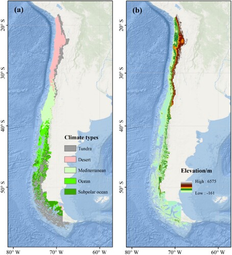
Chile has been chosen as the study area for manual interpretation testing because of its diverse land cover types and sufficient field data accumulation. Chile is located in South America, with complex topographic conditions, diverse climate types, and significant spatial variation in the natural environment. Under the influence of both topography and climate, Chile boasts rich natural vegetation types and biodiversity. According to the Köppen-Geiger climate classification system, Chile mainly consists of five major climate zones from north to south: tundra, desert, Mediterranean, marine, and sub-polar marine (Figure 1), and the climate varies greatly among climate zones. Due to the diverse climate and complex topography, Chile has a wide variety of land cover types.

Figure 1. The climate types (a) and topography (b) of Chile.

2.2. Preparation of ground truth samples and reference material

We chose 150 field samples of known land cover types evenly distributed in space as the ground truth to evaluate the performance of manual interpretation. The field samples are distributed in various climate areas, including the arid areas in the north, the Mediterranean center and the oceanic area in the south; ranging from the Atacama region to the Araucanía region. They cover eight first-level land cover types: croplands, forests, grasslands, shrublands, wetlands, water bodies, impervious surfaces, and barren lands. The satellite imagery used for manual interpretation includes ultra-high-resolution images from Google Earth and medium-high-resolution Landsat images with spectral curves from the Google Earth Engine (GEE) platform. For AI interpretation, the satellite imagery used was consistent with manual interpretation, and the DEM data used was NASA SRTM Digital Elevation 30 m.

Specific reference material assignments are described thereafter. For undergraduate and graduate students, we provided interpreters with interpretation reference material for each sample over five cycles of interpretation: (1) A series of ultra-high-resolution historical images from Google Earth (1985–2020); (2) Three ultra-high-resolution images of Google Earth in 2020 or similar years; (3) A Landsat 8 image (in false color composite) and the spectral profile of the target sample; (4) Short NDVI time series (2019–2020, Sentinel-2) and long-time series (2000–2020, Landsat). For high school students, the reference material for the two cycles of interpretation were: (1) a series of ultra-high-resolution historical images from Google Earth (1985–2020); (2) Three ultra-high-resolution images of Google Earth from 2020 or similar years. For AI interpretation, we inputted interpretation reference material into the model over 3 cycles: (1) a NASA SRTM Digital Elevation 30 m topographic image and a Landsat 8 image (in false color composite) in 2020; (2) a NASA SRTM Digital Elevation 30 m and an ultra-high-resolution images of Google Earth in 2020; (3) a NASA SRTM Digital Elevation 30 m topographic image, a Landsat 8 image (in false color composite) in 2020, an ultra-high-resolution images of Google Earth in 2020 and an NDVI of Landsat 8 image in 2020.

2.3. Image interpretation

In this study, a total of 50 interpreters participated in the remote sensing manual interpretation training. Thirty-two interpreters were undergraduate and graduate students from China Agricultural University. The other 18 interpreters were high school students from Beijing 35th Middle School. We chose deep learning as the representative of AI interpretation due to its powerful learning ability to automatically learn to complex patterns and laws through a large amount of data and iterative training.

In our study design, we used the interpretation performance of high school students as a benchmark to represent the image analysis ability of interpreters at the secondary educational level. The 32 undergraduate and graduate students represented interpreters at the higher educational level. They were randomly and equally divided into two groups. The analysis of 150 samples was repeated continuously for five cycles of manual interpretation. To compare with manual interpretation, we also used deep learning models as a proxy for AI interpretation. We conducted three rounds of experiments to have different number of samples interpreted by AI. They were as follows: (1) Small sample size: 50 samples, which were identical to human interpretations. The data is augmented to 1200 samples; (2) Medium sample size: 300 samples, augmented to 2400 samples; (3) Large sample size: 600 samples, augmented to 4800 samples. The datasets were divided into training and testing sets in a ratio of 8:2. The training sets were fed into Convolutional Neural Networks (CNNs) for image classification. The process of training and testing was illustrated in Figure 2.

Figure 2. Main reference and supporting information for each cycle of interpretation training and test.

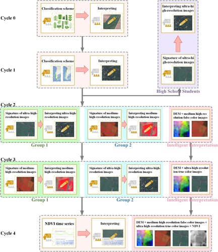
Cycle 0: There was only manual image interpretation in this cycle. According to the land cover composition of the study area, a third-level classification scheme was designed (see Table 1). Before manual interpretation, we provided a detailed explanation of the classification scheme to the interpreters. In this cycle, only the third-level land cover classification system of Chile was presented to the interpreters. This served as a blank control for the explanation.

Table 1. Land cover classification scheme.

Level 1	Level 2	Level 3
100 Croplands	110 Rice fields
	120 Greenhouse farming
	130 Herbaceous croplands
	140 Orchards	141 Woody orchards
		142 Vineyards
	150 Fallow
200 Forests	210 Broadleaf native forests
	220 Needle leaf native forests
	230 Mixed native forests
	240 Broadleaf plantations	241 Old plantation
		242 Clearcuts or young plantation
	250 Needle leaf plantations	251 Old plantation
		252 Clearcuts or young plantation
300 Grasslands	310 Pastures	311 Pasture, annual
		312 Pasture, perennial
	320 Other grasslands
	330 Grass, dry
400 Shrublands	410 Shrublands
	420 Shrubs and sparse trees mosaic
	430 Succulents
	440 Shrublands plantations
	450 Shrub, leaf-off
500 Wetlands	510 Marshland
	520 Mudflats
	530 Other wetlands
600 Water bodies	610 Lake
	620 Reservoir/pond
	630 River
	640 Ocean
700 Impervious surfaces
800 Barren lands	810 Dry salt flats
	820 Sandy areas
	830 Bare exposed rock	831 Rock
		832 Gravel
	840 Other barren lands

Cycle 1: There was only manual image interpretation in this cycle. This training cycle focused on providing background information on the climate and topography conditions in the study area (Fig 2). In this training, the elements of remote sensing manual interpretation were first briefly introduced. Then, a detailed presentation was given on the distribution of climate, topography, vegetation, and crops in the study area. For example, the forests near the Andes consist mainly of natural forests, while the forests in the western coastal mountain areas are more likely to be planted forests. The arid areas are primarily bare land with drought-resistant vegetation such as shrubs and cacti, and agricultural land in this arid climate zone is mainly found in river valleys. Central Chile experiences a typical Mediterranean climate with dry summers and wet winters, and crops and orchards are widely distributed in this climate zone.

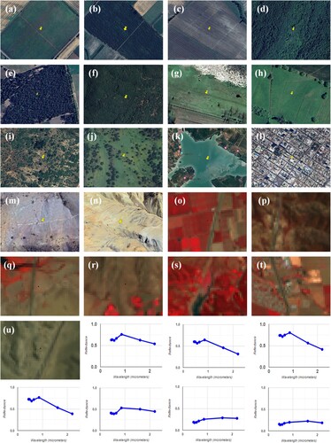
Cycle 2& Cycle 3: These two cycles contained AI interpretation. The second and third training sessions focused on interpreting land cover types using ultra-high and medium-high resolution remote sensing images. The ultra-high-resolution images were important reference material for manual interpretation (Tarko et al. 2021; Zhao et al. 2017). For manual interpretation, we held training on interpreting features and spectral curves of different land cover types in medium-high-resolution images, especially false color composite images. We provided a detailed explanation of the interpretation signatures for each land cover type in ultra-high-resolution (true color) images, such as WorldView, QuickBird, and IKONOS. This includes the interpretation signature for rice fields, forest plantations, and clear-cuts. Some examples of ultra-high and medium-high resolution (true and false color composite) images and spectral curves are shown in Figure 3. We trained a CNN model with two inputs for AI interpretation. The inputs of cycle 2 were DEM images and medium-high-resolution (false color composite) images. The inputs for cycle 3 were DEM images and ultra-high-resolution (true color) images.

Figure 3. Examples of ultra-high and medium-high resolution (true and false color composite) images and spectral curves. (a–c): The samples are of croplands, specifically rice fields (label = 110), woody orchards (label = 141), and vine-like orchards (label = 142) respectively. (d–f): The samples are of forests, including broadleaf native forest (label = 210), old needle-leaf plantation (label = 251), and mixed native forest (label = 230) respectively. (g–h): The samples consist of annual pasture (label = 311) and other grassland (label = 320). (i–j): The samples of shrublands (label = 410). (k): The reservoir sample (label = 620). (l): The sample of impervious surface (label = 800). (m–n): The samples are of barren lands, specifically dry salt flat (label = 910) and gravel (label = 932). (o–u): False color composite images and the curve at the bottom of each image represents the reflection spectrum curve of the central blue point. They are representative examples of croplands, forests, grasslands, shrublands, water bodies, impervious surfaces, and barren lands.

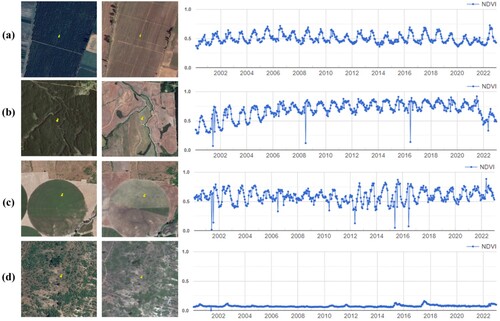
Cycle 4: This cycle also involved AI interpretation. The last cycle focused on training interpreters on how to interpret land cover using the supporting information provided by the time series of spectral indices. The NDVI is a crucial parameter that reflects vegetation growth and is commonly used in vegetation recognition. For manual interpretation, we presented interpreters with multi-year NDVI time series for various vegetation types, along with the precipitation time series as auxiliary information. For AI interpretation, we input DEM images, medium-high resolution (false color composite) images, ultra-high-resolution (true color) images, and NDVI images into the model to learn features from images from four different data sources. Through joint training, the model can synthesize this information to improve the classification performance. Some examples of NDVI time series are shown in Figure 4.

Figure 4. Examples illustrate the differences in NDVI time series between various vegetation types, such as croplands, forests, grasslands, and shrublands. (a–d): The samples of croplands, forests, grasslands, and shrublands.

2.4. Accuracy assessment

In this study, we developed a benchmark for comparing the correctness of an interpreter's labels with the true labels and used a confusion matrix to measure the interpreters’ performance in each class. Overall accuracy (OA) is calculated to evaluate the overall accuracy of interpretation. It is a basic evaluation metric. OA is the probability that all interpreters’ labels are the same as the true labels. If there is a true label with label = 141, and a certain interpreter provides an interpretation label with label = 140, then in the first and second-level classification systems, we believe it is correct; But in a more precise third-level classification system, we consider it is incorrect. By calculating the statistics of the confusion matrix and OA, we can comprehensively understand the performance of the classification model and effectively evaluate its classification performance on different classes. These evaluation indicators will help us objectively evaluate and compare the performance of the proposed method in practical applications. It is worth noting that we only consider consistency under the first-level classification system. If eight out of ten interpreters give a label of 100, then the consistency of this sample is 80%.

3. Results

3.1. Performance of interpreters with different educational levels

Interpretation accuracy performance may vary based on education level. To explore the differences in interpretation between them, in this study, we experimented with interpreters of different educational levels. Since only two manual interpretations were performed for the high school student group, the interpreter performance of interpreters in this section corresponds to the performance of the high school, undergraduate, and graduate student groups: (1) the accuracy of the blank control group when no reference material for manual interpretation is available, and (2) the accuracy of manual interpretation after training on all reference material.

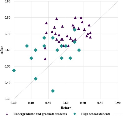
Figure 5 shows the interpretation accuracy for the first-level land cover types in the two manual interpretations. As expected, the interpretation accuracy for undergraduate and graduate students was significantly higher than that of high school students. With no prior experience in interpretation, high school students achieved an average interpretation accuracy of 52.22%, while undergraduate and graduate students achieved an interpretation accuracy of 61.13%. After training on all reference material, the average interpretation accuracy of the two groups of interpreters increased to 58.61% and 70.21%, respectively. The average interpretation accuracy increased by 6.39% and 9.08% for each group, respectively. No matter before or after the training, the interpretation accuracy is significantly higher for highly educated interpreters compared to those with a medium educational level. In addition, the training had a greater impact and resulted in greater improvement in interpretation accuracy for interpreters with higher education compared to high school students. Therefore, for most interpreters, interpreter training helps improve the accuracy of manual interpretation. Training was more effective for interpreters with higher educational levels.

Figure 5. Accuracy of different groups before and after training.

3.2. Performance of manual interpretation and AI interpretation after each cycle of training

To determine whether the accuracy of interpretation gradually improves with the number of training cycles, this study was conducted to statistically analyse the accuracy of manual interpretation and AI interpretation. Figure 6 illustrates the variations in interpretation accuracy and average accuracy of the third-level type and the first-level type during each interpretation cycle by two groups of interpreters. It can be observed from the figure that there were variations in the performance of the two groups of interpreters. However, the average interpretation accuracy showed a consistent improvement, indicating the effectiveness of visual training. When the classification scheme was very detailed, specifically under the third-level classification system, the interpretation accuracy was relatively low. Under the third-level classification system, the accuracy of the two groups was only 17.42% and 18.75% when the interpreters were not trained. However, after four cycles of training, the accuracy of both groups increased to 26.67% and 30.00% (see Figure 6(a–b)). Under the first-level classification system, the accuracy of both groups improved from 59.92% and 62.33% at the beginning to 68.67% and 71.75% after training (see Figure 7(c–d)). It can be observed that after a short period of visual training, the interpreters can recognize the first-level land cover types with greater accuracy. However, their ability to accurately identify the third-level land cover types may still be limited.

Figure 6. Changes in the accuracy of samples under third-level and first-level classification schemes.

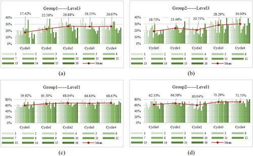
From Figure 6(a–c), it can be seen that the results of each training cycle were improved compared to the blank group (Cycle 0). Although in Figure 6(b), the accuracy of Cycle 2 was lower than that of Cycle 1, it was still higher than that of the blank group (Cycle 0). It is worth noting that in Figure 6(d), the accuracy of Cycle 2 was lower than that of Cycle 1, and it was also worse than that of the blank group. In training, when interpreters are exposed to ultra-high-resolution images before high-resolution images, it affects their interpretation. This is likely because interpreters struggle to adjust quickly to medium-high-resolution images with spectral curves after being exposed to clearer reference of ultra-high-resolution images. As a result, they become dependent on the ultra-high-resolution images. After training on medium-high-resolution images with spectral curves, the accuracy of most interpreters decreased (see Figure 6(a–c) Cycle 3, see Figure 6(b–d) Cycle 2).

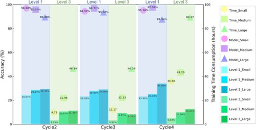
We designed three experimental cycles with varying sample sizes for the AI interpretation component. Figure 7 illustrated the accuracy and training time consumption of AI interpretation. The accuracies of AI interpretation for the three sample sizes were 23.77%, 27.33% and 30.78% for the first-level, and 4.0%, 10% and 10.77% for the third-level, respectively. It can be observed that the addition of reference material slightly improved the accuracy of the interpretation with the same input sample size. Similarly, as the training sample size increased, the accuracy improved for AI interpretation at different levels of refinement, but the training time consumption also increased exponentially. The training and interpretation time for manual interpretation in each cycle did not exceed 2 h. The average interpretation accuracy for the two groups of manual interpretation in the first-level type reached 66.08%, while for the third-level class, it reached 24.11%. From these results, it could be seen that the AI was inferior to humans in terms of accuracy and efficiency in the case of limited samples.

Figure 7. AI interpretation accuracy and its training time consumption.

3.3. Performance of interpretation with different reference material

We conducted a series of experiments focusing on the interpretation performance of different reference material. We selected herbaceous croplands (label = 130), woody orchards (label = 141), natural forests (label = 210 / 220), forest plantations (label = 241 / 251), grasslands (label = 311 / 320), and shrublands (label = 410 / 420 / 440) as examples to investigate the responsiveness of different vegetation types to various reference material. These classes were chosen because of their large sample sizes and the potential for confusion between samples. We calculated the degree of improvement in manual interpretation accuracy for the vegetation types mentioned above after all interpreters received four cycles of interpretation training. The sensitivities were categorized as follows: If the addition of a new reference did not enhance to the accuracy of interpreting a vegetation class, the interpretation accuracy of this vegetation type was considered insensitive to this new knowledge. If the improvement in accuracy was less than 8%, the interpretation accuracy of this vegetation type was considered sensitive to this new reference. If the accuracy improved by 8% or more, the interpretation accuracy of this vegetation type was considered very sensitive to this new reference. The classes of sensitivity are shown in Table 2.

Table 2. Sensitivity to reference material.

Accuracy improvement (ϵ)	Value	Sensibility
ϵ ≤ 0	1	Insensitive
0 < ϵ ≤ 8%	2	Sensitive
ϵ > 8%	3	Very sensitive

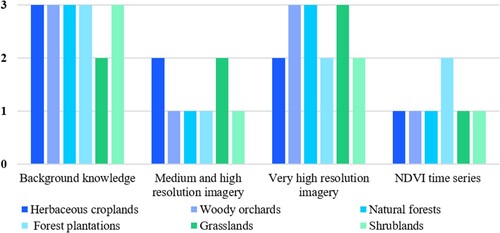
Figure 8 shows the sensitivity of the six vegetation types mentioned above to four reference material: ‘the background information of the study area,’ ‘the medium-high-resolution images with spectral curves,’ ‘the ultra-high-resolution images,’ and ‘NDVI time series.’ We found that:

1. The six vegetation types mentioned above show the highest sensitivity to background information and the lowest sensitivity to NDVI time series knowledge. Interpretation of ultra-high-resolution images contributes to improving the accuracy of vegetation interpretation.

2. The vegetation types sensitive to the background information of the study area include herbaceous croplands, woody orchards, natural forests, forest plantations, shrublands, and grasslands, which were found to be the most sensitive. The background information is extremely helpful in accurately identifying herbaceous croplands, forest plantations, and shrubland in all reference material.

3. The interpretation signatures of medium-high-resolution images with spectral curves had a positive effect on correctly identifying herbaceous croplands and grasslands, but their contribution to identifying other classes was not significant.

4. Woody orchards, natural forests, and grasslands were highly sensitive indicators in the interpretation of ultra-high-resolution images. Among all the reference material, this particular reference was the most helpful in accurately identifying grasslands.

5. In this study, it was found that, except for forest plantations, all other vegetation types showed no sensitivity to the NDVI time series information. This suggests that incorporating NDVI time series information did not contribute to enhancing the accuracy of manual interpretation for interpreters.

Figure 8. Sensitivity of several vegetation types to reference material.

The result shows that choosing appropriate reference material has an important impact on interpreting performance. By comparison, we found that interpreters using ultra-high-resolution images for reference performed best.

3.4. The relationship between group consistency and interpretation accuracy

From the above analysis, it can be concluded that through training and manual interpretation, interpreters can relatively accurately identify the first-level land cover types. To better evaluate the group performance of undergraduate and graduate student interpreters, this part evaluated the first and last cycle of interpretation samples separately. Among the labels provided by 32 undergraduate and graduate interpreters for each sample, the most consistent type was the type after integrating opinions, referred to as the ‘group interpretation type’. For instance, in the case of the sample with id = 7, 24 out of the 32 interpreters identified it as ‘woody orchard’. Therefore, the third-level group interpretation type for this sample was ‘woody orchard’, while the first-level group interpretation type was ‘farmland’. The consistency for this interpretation was 0.75, corresponding to column 0.7 in Figure 9.

Figure 9. Accuracy of the most consistent land cover types.

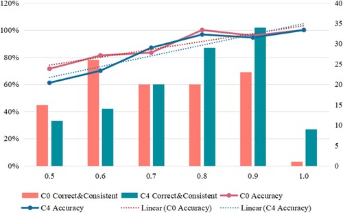
Figure 9 shows the accuracy for the group interpreting type, with the dashed line representing the fitted trend. As can be seen from the figure, the higher the consistency, the greater the interpretation accuracy. However, even group interpreting types can be incorrect, so this study further analysed the confusion between group interpreting types and authentic types (Tables 3 and 4). The overall accuracy of the cycle0 group sample was 76.67%, and the OA improved to 80.67% after four complete training cycles. Figure 10 shows several sample examples that may be confusing, such as cropland, grassland, plantation, shrub types, and water bodies. It also displays the reflectance spectrum curves of the aforementioned types, along with the long-term NDVI from 2000 to 2020 and the short-term NDVI curve from 2019 to 2020. The two-types confusion matrix revealed a high level of confusion between cropland and grassland samples, with a significant number of grassland samples misclassified as cropland. The annual grassland and herbaceous cropland were very similar, and in the NDVI time series information, the differences between the two types were also minimal, leading to easy confusion.Herbaceous cropland was mostly irrigated, and its water content was higher than that of pasture land. These differences can be observed in the spectral curve. In addition, annual grasses have longer growing seasons (Fig.10a-b). Confusion between woodlands and shrubs mainly occurred in the case of plantations, due to the obvious and regular texture of plantations, which caused tree plantations in the ultra-high-resolution images to appear similar to shrub plantations. Additionally, the shrub samples in this study were mostly found in arid areas with a lower NDVI than in woodlands.

Figure 10. Examples of confusing samples. (a–d): The samples include croplands (herbaceous cropland), grasslands (annual pasture), forests (broadleaf plantation), and shrublands (shrubland plantation). (e–f): Water bodies in different seasons or years.

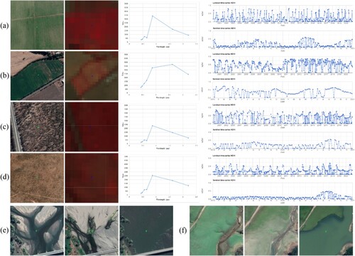
Table 3. Cycle0: The confusion matrix of the most consistent and true land cover types.

First-level type label		Cycle1: The most consistent types
		100	200	300	400	500	600	700	800
True types	100	47	5	6	0	0	0	0	0
	200	1	38	0	4	0	0	0	0
	300	1	0	11	1	1	0	0	0
	400	2	4	0	12	0	0	0	0
	500	0	0	0	0	0	0	0	1
	600	0	0	0	0	0	1	0	0
	700	0	0	0	0	0	0	1	0
	800	0	0	0	1	0	0	0	5

Table 4. Cycle 4: The confusion matrix of the most consistent and true land cover types.

First-level type label		Cycle4: The most consistent types
		100	200	300	400	500	600	700	800
True types	100	46	3	5	0	0	0	0	0
	200	1	39	1	1	0	0	0	0
	300	4	1	14	3	0	0	0	0
	400	0	5	0	14	0	0	0	0
	500	0	0	2	0	1	1	0	1
	600	0	0	0	0	0	1	0	0
	700	0	0	0	0	0	0	2	0
	800	0	0	0	1	0	0	0	4

In addition, there were significant differences in the NDVI values between shrub forests during the growing season and the non-growing season (Figure 9(c–d)). It was generally accepted that water bodies were easily identifiable in both high- and medium-high-resolution images and that water bodies exhibited pronounced seasonal variations as a land-cover type (see Figure 9). In the study, the interpreters were provided with reference images of ultra-high resolution. However, these images were not taken during the flood season, which could explain why the water samples were mislabeled.

4. Discussions

4.1. Interpretation performance

In this study, we observed that untrained interpreters performed poorly in land cover interpretation. However, after interpretation training, the interpretation accuracy of both high school students and undergraduate/graduate students improved, especially the performance improvement of interpreters with higher education levels is more significant, showing a positive relationship. This highlights the positive impact of training on interpreter performance and suggests a correlation between educational level and interpretive ability. When comparing the contributions of different reference material to image interpretation, we found that using ultra-high-resolution images as reference material had the most significant effect on improving interpretation accuracy, followed by background information of the study area and NDVI time series. This provides guidance for detailing various reference material during training, emphasizing the criticality of reference material selection in improving interpreter skills. In addition, vegetation types are sensitive to the support provided by ultra-high-resolution images, suggesting that the characteristics of different vegetation types need to be considered during the training process to better interpret the images. This has practical implications for land cover interpretation for different regions and vegetation types. More than 50% of the interpreters agree on the label, and the accuracy of the label can reach 88.64%. Therefore, when we have a sample dataset labeled by various volunteers but without validation by experts or field surveys, we can consider the land cover type agreed upon by the majority as the true label and the level of agreement as the reliability of this label. The more consistently the samples were labeled, the more likely they were to be correct. Finally, the study found that as the number of training cycles increases, the increment of interpretation accuracy gradually decreases, which may be affected by human mental fatigue. Therefore, it is recommended to reasonably plan the number and duration of training cycles to reduce the mental fatigue of interpreters. This has practical implications for keeping interpreters focused and improving productivity.

The accuracy and efficiency of AI interpretation fell short of expectations, possibly due to several reasons. Firstly, the model might have been trained on a limited dataset, hindering its ability to learn diverse patterns. While this study utilized only thousands of samples, deep learning models commonly train on millions. Secondly, the model's architecture may not have been sufficiently complex to capture intricate patterns in the data. Conversely, overly complex architectures can lead to overfitting. Thus, selecting an optimal model architecture is crucial for improving accuracy. Lastly, improper tuning of hyperparameters could have affected performance. Although suitable hyperparameters were chosen through experiment comparison, further optimization is still possible.

4.2. Reference material

In this study, we delve into the characteristics and contributions of different reference material in land cover interpretation. Research indicates that background knowledge and ultra-high-resolution images of the study area can provide rich spatial details of land cover, aiding in distinguishing easily confused land cover types. This is particularly crucial for fine-grained land cover interpretation. In areas where ultra-high-resolution images are available, we recommend prioritizing their use as reference material. Furthermore, the study revealed that the accuracy of explanations increased when background knowledge served as reference material. If there is a lack of ultra-high-resolution imagery in the study area, the study recommends providing interpreters with background knowledge to better understand land cover. The false-color composite of medium-high-resolution imagery can provide a more enhanced visualization of the spectral curve.

The study also found that the introduction of NDVI reference material can improve the accuracy of third-level types in AI interpretation, especially in identifying similar vegetation types. In our study, we clearly observed poor accuracy under the third-level classification system. Although the reference material mentioned above can effectively improve the accuracy under the first-level classification system, more useful reference material, such as vegetation indices, need to be explored to help interpreters recognize finer land cover classes. Long- and short-term NDVI time series can respectively reflect the inter-annual and intra-annual variations in the growth state of vegetation. For example, short-term NDVI time series reflect the seasonal variation of vegetation within a year, making them more useful for interpreting annual vegetation, such as herbaceous crops. Long-term NDVI time series show the approximate planting and cutting times of perennial vegetation, providing a valuable reference for identifying orchards and forest plantations.

4.3. Consistency of interpreting

When there were sample datasets labeled by different volunteers but not validated by experts or field surveys, the most consistent land cover type (with the type explained by the group as the type label) could be used, and the degree of agreement was considered the reliability of that label. However, there were also some errors in the labeling of the group samples, particularly in distinguishing between herbaceous cropland and annual grassland. These types were often mislabeled even on high-resolution images. Therefore, it was necessary to utilize additional reference material, such as reflectance spectrum curves and growing season lengths, to make more accurate comparisons for these confusing types.

4.4. Limitations and future work

For the first time in our study, the inclusion of medium-high-resolution images with spectral curves did not significantly enhance the interpretation accuracy. This discrepancy may stem from interpreters relying too heavily on high-resolution images, thereby limiting the utility of spectral curves. Therefore, a bold hypothesis is proposed: whether providing only spectral curves for interpretation would yield different results. Secondly, interpreters should document the self-assessed uncertainty of the samples and then receive specialized training for types with higher uncertainty. To enhance the accuracy of interpretation in the third-level classification system, it is also crucial to incorporate expert reviews. After the interpretation is completed, the interpreted material are given to experts for calibration. The expert compares the labeling results of each sample and determines their consistency. Samples with low consistency are corrected or relabeled to ensure the accuracy and reliability of labeling. The feedback provided during the interpretation process can help reduce uncertainty and confusion in subsequent interpretations (Tarko et al. 2021). In addition, to further evaluate the reliability of interpretation, it is possible to calculate the consistency of each type, which represents the percentage of agreement among volunteers when interpreting specific types. This can help us identify types that are confusing or controversial, and thus pay more attention to the correct labeling of these types. Then, the quality of the references provided in this study is high, so the relationship between the quality of the references and the accuracy can be explored in the future (Foody 2009; Stehman and Foody 2019; Wickham et al. 2021). Finally, some land cover types of samples may change seasonally in practical applications. Inevitably, some samples may be affected by seasonal changes in land cover types. For example, during the dry season, water bodies may appear as grasslands, leading to uncertainties in interpretation. Interpreters need to refer to multi-temporal material. Within time and cost constraints, labeling as many sample types as possible in each time phase is advisable. If it is only necessary to determine the composite label of a sample within a year, it is important to specify which type takes priority, such as following the principles of ‘greenest’ and ‘wettest’ (Zhao et al. 2016). By utilizing multi-temporal material, interpreters can assign land cover classifications at different periods, which is beneficial for generating multi-seasonal land cover maps.

5. Conclusions

In this study, we invited 50 interpreters to complete five cycles of manual image interpretation after being trained and provided with different supporting material. In addition, a comparison between AI interpretation and manual interpretation with varying numbers of sample inputs was also set up. After evaluating the interpretation accuracies achieved by various groups of volunteers and across different cycles, we can draw the following conclusions: First, volunteers with higher educational backgrounds perform better in interpreting land cover types from remotely sensed imagery. Second, the manual interpretation accuracies increased gradually after being trained and provided with more supporting material. Among the various supporting material, the ultra-high-resolution images and the background knowledge of the study area contributed the most to accuracy improvement, while the NDVI time series contributed the least. The performance of the machine learning algorithm, represented by a CNN model, was inferior to the performance of manual interpretation by human beings when they were both trained by a small sample dataset. Third, the interpretation accuracies of some land cover types are more sensitive than others to specific supporting material. For example, NDVI time series were very helpful in the interpretation of forest plantations. Fourth, group consistency was a good indicator of the reliability of samples collected by various volunteers.

The findings of our research provide guidance in collecting high-quality land cover training and validation samples through crowdsourcing. To ensure the quality of the samples collected through manual image interpretation, we recommend inviting educated volunteers, providing necessary training, preparing effective supporting material, and filtering samples based on group consistency. Although manual image interpretation is time-consuming and labor-intensive, it offers clear advantages over AI interpretation, which is trained with few samples, especially in complex scenes with limited training data for machine learning algorithms. Human cognition enables informed decisions even with sparse data, whereas AI relies heavily on abundant training samples. Thus, manual interpretation remains preferred for its adaptability and expertise across diverse environments. Despite the challenges associated with AI interpretation mentioned above, integrating it with manual interpretation offers a promising solution for land cover sample collection. We can first analyse the image with AI to provide recommended answers for the volunteers, and also accumulate more basic samples of good quality for training the AI models , achieving a more comprehensive and accurate interpretation.

In future research, our main goal is to provide a more comprehensive reference for handling ambiguous land cover types to support interpreters in completing their tasks more efficiently. We plan to conduct in-depth exploration of the most suitable reference material in specific scenarios to ensure the superiority of the training program in terms of comprehensiveness, pertinence and effectiveness. Additionally, we will study the relationship between a larger number of samples and interpretation accuracy to determine the appropriate training sample size required to achieve manual interpretation levels of model explanation performance (Li et al. 2023; Ramezan et al. 2021). This series of research goals aims to further improve the quality and reliability of land cover interpretation. Ultimately, we believe these efforts will not only improve the quality of interpretations but also effectively expand the sample base. This provides powerful guidance for future land cover research and interpretation, and promotes our deeper understanding and response to changes in the earth's surface.

Disclosure statement

No potential conflict of interest was reported by the author(s).

Data availability statement

Data sharing is not applicable to this article as no new data were created or analyzed in this study.

Additional information

Funding

This research was funded by the National Natural Science Foundation of China [grant number 42001352], the National Key Research and Development Program of China “study on farmland utilization dynamic monitoring and grain Productivity Evaluation Technology” [grant number 2022YFB3903504].

References

- AbdelRahman, Mohamed AE. 2023. “An Overview of Land Degradation, Desertification and Sustainable Land Management Using GIS and Remote Sensing Applications.” Rendiconti Lincei. Scienze Fisiche e Naturali 34 (3): 767–808.
- Bah, Mamadou Dian, Adel Hafiane, and Raphael Canals. 2023. “Hierarchical Graph Representation for Unsupervised Crop row Detection in Images.” Expert Systems with Applications 216: 119478. https://doi.org/10.1016/j.eswa.2022.119478.
- Bai, Ruyue, Zegen Wang, Heng Lu, Chen Chen, Xiuju Liu, Guohao Deng, Qiang He, Zhiming Ren, Bin Ding, and Xin Ye. 2023. “Earthquake-Triggered Landslide Interpretation Model of High Resolution Remote Sensing Imageries Based on Bag of Visual Word.” Earthquake Research Advances 3 (2): 100196. https://doi.org/10.1016/j.eqrea.2022.100196.
- Cengiz, A. V. C. I., Muhammed Budak, Nur Yağmur, and Filiz Balçik. 2023. “Comparison Between Random Forest and Support Vector Machine Algorithms for LULC Classification.” International Journal of Engineering and Geosciences 8 (1): 1–10. https://doi.org/10.26833/ijeg.987605.
- Das, Niladri, Prolay Mondal, Subhasish Sutradhar, and Ranajit Ghosh. 2021. “Assessment of Variation of Land use/Land Cover and its Impact on Land Surface Temperature of Asansol Subdivision.” The Egyptian Journal of Remote Sensing and Space Science 24 (1): 131–149. https://doi.org/10.1016/j.ejrs.2020.05.001.
- Dimitrovski, Ivica, Ivan Kitanovski, Dragi Kocev, and Nikola Simidjievski. 2023. “Current Trends in Deep Learning for Earth Observation: An Open-Source Benchmark Arena for Image Classification.” ISPRS Journal of Photogrammetry and Remote Sensing 197: 18–35. https://doi.org/10.1016/j.isprsjprs.2023.01.014.
- Foody, Giles M. 2009. “The Impact of Imperfect Ground Reference Data on the Accuracy of Land Cover Change Estimation.” International Journal of Remote Sensing 30 (12): 3275–3281. https://doi.org/10.1080/01431160902755346.
- Foody, Giles, Gavin Long, Michael Schultz, and Ana-Maria Olteanu-Raimond. 2022. “Assuring the Quality of VGI on Land Use and Land Cover: Experiences and Learnings from the LandSense Project.” Geo-spatial Information Science 27 (1): 16–37. https://doi.org/10.1080/10095020.2022.2100285.
- Fraisl, Dilek, Gerid Hager, Baptiste Bedessem, Margaret Gold, Pen-Yuan Hsing, Finn Danielsen, Colleen B. Hitchcock, et al. 2022. “Citizen Science in Environmental and Ecological Sciences.” Nature Reviews Methods Primers 2 (1): 64. https://doi.org/10.1038/s43586-022-00144-4.
- Hussain, Sajjad, Muhammad Mubeen, Ashfaq Ahmad, Hamid Majeed, Saeed Ahmad Qaisrani, Hafiz Mohkum Hammad, Muhammad Amjad, Iftikhar Ahmad, Shah Fahad, and Naveed Ahmad. 2023. “Assessment of Land Use/Land Cover Changes and Its Effect on Land Surface Temperature Using Remote Sensing Techniques in Southern Punjab, Pakistan.” Environmental Science and Pollution Research 30 (44): 99202–99218. https://doi.org/10.1007/s11356-022-21650-8.
- Janowicz, Krzysztof, Song Gao, Grant McKenzie, Yingjie Hu, and Budhendra Bhaduri. 2020. “GeoAI: Spatially Explicit Artificial Intelligence Techniques for Geographic Knowledge Discovery and Beyond.” International Journal of Geographical Information Science 34 (4): 625–636.
- Jiao, Licheng, Zhongjian Huang, Xu Liu, Yuting Yang, Mengru Ma, Jiaxuan Zhao, Chao You, et al. 2023. “Brain-Inspired Remote Sensing Interpretation: A Comprehensive Survey.” IEEE Journal of Selected Topics in Applied Earth Observations and Remote Sensing 16: 2992–3033. https://doi.org/10.1109/JSTARS.2023.3247455.
- Kim, Wonjik, Asako Kanezaki, and Masayuki Tanaka. 2020. “Unsupervised Learning of Image Segmentation Based on Differentiable Feature Clustering.” IEEE Transactions on Image Processing 29: 8055–8068. https://doi.org/10.1109/TIP.2020.3011269.
- Kohli, Divyani, Alfred Stein, and Richard Sliuzas. 2016. “Uncertainty Analysis for Image Interpretations of Urban Slums.” Computers, Environment and Urban Systems 60: 37–49. https://doi.org/10.1016/j.compenvurbsys.2016.07.010.
- Krabina, Bernhard. 2023. “Building a Knowledge Graph for the History of Vienna with Semantic MediaWiki.” Journal of Web Semantics 76: 100771. https://doi.org/10.1016/j.websem.2022.100771.
- Kraff, N. J., M. Wurm, and H. Taubenbck. 2020. “Uncertainties of Human Perception in Visual Image Interpretation in Complex Urban Environments.” IEEE Journal of Selected Topics in Applied Earth Observations and Remote Sensing 13 (PP): 4229–4241. https://doi.org/10.1109/JSTARS.2020.3011543.
- Latifovic, Rasim, Darren Pouliot, and Ian Olthof. 2017. “Circa 2010 Land Cover of Canada: Local Optimization Methodology and Product Development.” Remote Sensing 9: 1098. https://doi.org/10.3390/rs9111098.
- Lesiv, Myroslava, Linda See, Juan Carlos Laso Bayas, Tobias Sturn, Dmitry Schepaschenko, Mathias Karner, Inian Moorthy, Ian McCallum, and Steffen Fritz. 2018. “Characterizing the Spatial and Temporal Availability of Very High Resolution Satellite Imagery in Google Earth and Microsoft Bing Maps as a Source of Reference Data.” Land 7 (4): 118.
- Li, Chenxi, Zaiying Ma, Liuyue Wang, Weijian Yu, Donglin Tan, Bingbo Gao, Quanlong Feng, Hao Guo, and Yuanyuan Zhao. 2021. “Improving the Accuracy of Land Cover Mapping by Distributing Training Samples.” Remote Sensing 13 (22): 4594. https://doi.org/10.3390/rs13224594.
- Li, Wenwen, Sizhe Wang, Xiao Chen, Yuanyuan Tian, Zhining Gu, Anna Lopez-Carr, Andrew Schroeder, Kitty Currier, Mark Schildhauer, and Rui Zhu. 2023. “Geographvis: A Knowledge Graph and Geovisualization Empowered Cyberinfrastructure to Support Disaster Response and Humanitarian aid.” ISPRS International Journal of Geo-Information 12 (3): 112. https://doi.org/10.3390/ijgi12030112.
- Li, Linhui, Wenjun Zhang, Xiaoyan Zhang, Mahmoud Emam, and Weipeng Jing. 2023. “Semi-supervised Remote Sensing Image Semantic Segmentation Method Based on Deep Learning.” Electronics 12 (2): 348. https://doi.org/10.3390/electronics12020348.
- Liu, Yu, Jingtao Ding, Yanjie Fu, and Yong Li. 2023. “UrbanKG: An Urban Knowledge Graph System.” ACM Transactions on Intelligent Systems and Technology 14 (4): 1–25.
- Lv, Ning, Zenghui Zhang, Cong Li, Jiaxuan Deng, Tao Su, Chen Chen, and Yang Zhou. 2023. “A Hybrid-Attention Semantic Segmentation Network for Remote Sensing Interpretation in Land-Use Surveillance.” International Journal of Machine Learning and Cybernetics 14 (2): 395–406. https://doi.org/10.1007/s13042-022-01517-7.
- Maxwell, Aaron E., Timothy A. Warner, and Fang Fang. 2018. “Implementation of Machine-Learning Classification in Remote Sensing: An Applied Review.” International Journal of Remote Sensing 39 (9): 2784–2817. https://doi.org/10.1080/01431161.2018.1433343.
- McRoberts, Ronald E., Stephen V. Stehman, Greg C. Liknes, Erik Næsset, Christophe Sannier, and Brian F. Walters. 2018. “The Effects of Imperfect Reference Data on Remote Sensing-Assisted Estimators of Land Cover Class Proportions.” ISPRS Journal of Photogrammetry and Remote Sensing 142: 292–300. https://doi.org/10.1016/j.isprsjprs.2018.06.002.
- Papoutsis, Ioannis, Nikolaos Ioannis Bountos, Angelos Zavras, Dimitrios Michail, and Christos Tryfonopoulos. 2023. “Benchmarking and Scaling of Deep Learning Models for Land Cover Image Classification.” ISPRS Journal of Photogrammetry and Remote Sensing 195: 250–268. https://doi.org/10.1016/j.isprsjprs.2022.11.012.
- Raja, Piyush, Santosh Kumar, Digvijay Singh Yadav, Amit Kumar, and Ram Krishna Kumar. 2023. “Intelligent Remote Sensing: Applications and Techniques.” Journal of Image Processing and Intelligent Remote Sensing (JIPIRS) ISSN 2815-0953 3 (02): 46–53.
- Ramezan, Christopher A., Timothy A. Warner, Aaron E. Maxwell, and Bradley S. Price. 2021. “Effects of Training Set Size on Supervised Machine-Learning Land-Cover Classification of Large-Area High-Resolution Remotely Sensed Data.” Remote Sensing 13 (3): 368. https://doi.org/10.3390/rs13030368.
- Roy, David P., Haiyan Huang, Rasmus Houborg, and Vitor S. Martins. 2021. “A Global Analysis of the Temporal Availability of PlanetScope High Spatial Resolution Multi-Spectral Imagery.” Remote Sensing of Environment 264: 112586. https://doi.org/10.1016/j.rse.2021.112586.
- Sadeghi, Fatemeh, Ata Larijani, Omid Rostami, Diego Martín, and Parisa Hajirahimi. 2023. “A Novel Multi-Objective Binary Chimp Optimization Algorithm for Optimal Feature Selection: Application of Deep-Learning-Based Approaches for SAR Image Classification.” Sensors 23 (3): 1180. https://doi.org/10.3390/s23031180.
- Schepaschenko, Dmitry, Linda See, Myroslava Lesiv, Jean-François Bastin, Danilo Mollicone, Nandin-Erdene Tsendbazar, Lucy Bastin, Ian McCallum, Juan Carlos Laso Bayas, and Artem Baklanov. 2019. “Recent Advances in Forest Observation with Visual Interpretation of Very High-Resolution Imagery.” Surveys in Geophysics 40: 839–862.
- Seyam, Md Mahadi Hasan, Md Rashedul Haque, and Md Mostafizur Rahman. 2023. “Identifying the Land use Land Cover (LULC) Changes Using Remote Sensing and GIS Approach: A Case Study at Bhaluka in Mymensingh, Bangladesh.” Case Studies in Chemical and Environmental Engineering 7: 100293. https://doi.org/10.1016/j.cscee.2022.100293.
- Stehman, Stephen. V, and Giles. M Foody. 2019. “Key Issues in Rigorous Accuracy Assessment of Land Cover Products.” Remote Sensing of Environment 231: 111199. https://doi.org/10.1016/j.rse.2019.05.018.
- Tariq, Aqil, Jianguo Yan, Alexandre. S Gagnon, Mobushir Riaz Khan, and Faisal Mumtaz. 2023. “Mapping of Cropland, Cropping Patterns and Crop Types by Combining Optical Remote Sensing Images with Decision Tree Classifier and Random Forest.” Geo-spatial Information Science 26 (3): 302–320. https://doi.org/10.1080/10095020.2022.2100287.
- Tarko, A., N. E. Tsendbazar, S. de Bruin, and A. K. Bregt. 2020. “Influence of Image Availability and Change Processes on Consistency of Land Transformation Interpretations.” International Journal of Applied Earth Observation and Geoinformation 86: 102005. https://doi.org/10.1016/j.jag.2019.102005.
- Tarko, Agnieszka, Nandin-Erdene Tsendbazar, Sytze de Bruin, and Arnold K. Bregt. 2021. “Producing Consistent Visually Interpreted Land Cover Reference Data: Learning from Feedback.” International Journal of Digital Earth 14 (1): 52–70. https://doi.org/10.1080/17538947.2020.1729878.
- Tavra, Marina, Ivan Racetin, and Josip Peroš. 2021. “The Role of Crowdsourcing and Social Media in Crisis Mapping: A Case Study of a Wildfire Reaching Croatian City of Split.” Geoenvironmental Disasters 8 (1): 10. https://doi.org/10.1186/s40677-021-00181-3.
- Van Coillie, Frieke M. B., Soetkin Gardin, Frederik Anseel, Wouter Duyck, Lieven P. C. Verbeke, and Robert R. De Wulf. 2014. “Variability of Operator Performance in Remote-Sensing Image Interpretation: The Importance of Human and External Factors.” International Journal of Remote Sensing 35 (2): 754–778. https://doi.org/10.1080/01431161.2013.873152.
- Waldner, François, Anne Schucknecht, Myroslava Lesiv, Javier Gallego, Linda See, Ana Pérez-Hoyos, Raphaël d'Andrimont, Thomas De Maet, Juan Carlos Laso Bayas, and Steffen Fritz. 2019. “Conflation of Expert and Crowd Reference Data to Validate Global Binary Thematic Maps.” Remote Sensing of Environment 221: 235–246.
- Wang, Zhipan, Di Liu, Zhongwu Wang, Xiang Liao, and Qingling Zhang. 2023. “A New Remote Sensing Change Detection Data Augmentation Method Based on Mosaic Simulation and Haze Image Simulation.” IEEE Journal of Selected Topics in Applied Earth Observations and Remote Sensing 16: 4579–4590.
- Watkinson, Kirsty, Jonathan J. Huck, and Angela Harris. 2023. “Using Gamification to Increase map Data Production During Humanitarian Volunteered Geographic Information (VGI) Campaigns.” Cartography and Geographic Information Science 50 (1): 79–95. https://doi.org/10.1080/15230406.2022.2156389.
- Wickham, James, Stephen. V Stehman, Daniel G Sorenson, Leila Gass, and Jon A Dewitz. 2021. “Thematic Accuracy Assessment of the NLCD 2016 Land Cover for the Conterminous United States.” Remote Sensing of Environment 257: 112357. https://doi.org/10.1016/j.rse.2021.112357.
- Xu, Rongtao, Changwei Wang, Jiguang Zhang, Shibiao Xu, Weiliang Meng, and Xiaopeng Zhang. 2023. “Rssformer: Foreground Saliency Enhancement for Remote Sensing Land-Cover Segmentation.” IEEE Transactions on Image Processing 32: 1052–1064. https://doi.org/10.1109/TIP.2023.3238648.
- Zhang, Ce, Isabel Sargent, Xin Pan, Huapeng Li, Andy Gardiner, Jonathon Hare, and Peter M. Atkinson. 2018. “An Object-Based Convolutional Neural Network (OCNN) for Urban Land Use Classification.” Remote Sensing of Environment 216: 57–70. https://doi.org/10.1016/j.rse.2018.06.034.
- Zhang, Zhan, Mi Zhang, Jianya Gong, Xiangyun Hu, Hanjiang Xiong, Huan Zhou, and Zhipeng Cao. 2023. “LuoJiaAI: A Cloud-Based Artificial Intelligence Platform for Remote Sensing Image Interpretation.” Geo-spatial Information Science 26 (2): 218–241.
- Zhao, Yuanyuan, Duole Feng, Durai Jayaraman, Daniel Belay, Heiru Sebrala, John Ngugi, Eunice Maina, et al. 2018. “Bamboo Mapping of Ethiopia, Kenya and Uganda for the Year 2016 Using Multi-Temporal Landsat Imagery.” International Journal of Applied Earth Observation and Geoinformation 66: 116–125. https://doi.org/10.1016/j.jag.2017.11.008.
- Zhao, Yuanyuan, Duole Feng, Le Yu, Linda See, Steffen Fritz, Christoph Perger, and Peng Gong. 2017. “Assessing and Improving the Reliability of Volunteered Land Cover Reference Data.” Remote Sensing 9: 10. https://doi.org/10.3390/rs9101034.
- Zhao, Yuanyuan, Duole Feng, Le Yu, Xiaoyi Wang, Yanlei Chen, Yuqi Bai, H. Jaime Hernández, et al. 2016. “Detailed Dynamic Land Cover Mapping of Chile: Accuracy Improvement by Integrating Multi-Temporal Data.” Remote Sensing of Environment 183: 170–185. https://doi.org/10.1016/j.rse.2016.05.016.