Impact of spatially-dense in-situ observations on ocean forecasts of mixed layer and thermocline depth

ABSTRACT

Ocean models, such as the Navy Coastal Ocean Model (NCOM), rely on ocean observations through data assimilation to predict the evolution of ocean phenomena accurately. The accuracy is highly dependent on the type and quantity of observations available. This work attempts to examine the impact of spatially dense in-situ profile observations on the forecasts of mixed layer depth (MLD) and thermocline depth (TD), using a three-dimensional variational data assimilation algorithm. To do this, a twin data assimilation experiment is used to simulate the impact of float deployments on the forecast of MLD and TD in a specific area of interest (AOI) of the North Atlantic. It is found that during the northern hemisphere summer the model MLD is sensitive to the sea surface temperature (SST) observations rather than the profiling floats. TD is more strongly impacted by the assimilation of float observations, and the experiment with the most floats produces the best results. During the northern hemisphere winter the profiling floats have a greater impact on the model simulation of MLD. Finally, the overall lack of substantial improvement in the winter months for the highest density of profiling floats is determined to be due to the data assimilation methodology itself.

1. Introduction

Features such as the mixed layer depth (MLD) and thermocline depth (TD) are important to capture in ocean modelling. MLD is the depth of the bottom of the mixed layer of the ocean, which is a region extending from the surface of the ocean to some depth exhibiting nearly constant temperature or density, depending on the definition; the uniform temperature within this layer is due to the turbulent mixing that characterises this layer (Helber et al. 2008). The thermocline, on the other hand, is the region (typically under the mixed layer) where the temperature rapidly decreases with depth. For the purpose of this work, the thermocline depth is defined as the deepest base of the thermocline where the temperature ceases to decrease rapidly with depth and the water column becomes isothermal. Ocean models, such as the regional Navy Coastal Ocean Model (NCOM; Barron et al. 2006) or the global HYbrid Coordinate Ocean Model (HYCOM; Bleck 2002), can realistically represent these features, however, precise prediction requires an accurate model initial state derived from observations. The ocean is significantly under sampled in both space and time. Therefore, thoughtful design of the observing strategy in terms of the number, deployment, and type of sensor is important. The experiments to be shown here seek to illuminate the impact of in-situ observations on the ocean model forecast of MLD and TD, for one specific case. Conducting actual field experiments in order to examine the impact of sensor deployment for a given region and set of metrics is prohibitive, both in terms of cost (in materials and personnel) and time. Therefore, a model-based examination known as a twin data assimilation method is used here.

A twin data assimilation method is similar to an observing system simulation experiment (OSSE) and is a tool that can be used when evaluating a model, observing system, or data assimilation method (Halliwell et al. 2014; Zeng et al. 2020). In this work, the twin data assimilation test is comprised of two components: the model-based ‘nature’ run and the ‘assimilative’ run. The nature run (NR) is intended to act as the surrogate real ocean for the experiments to be conducted. It should be of sufficient spatial and temporal resolution in order to realistically represent the dynamics of the real ocean and simulate features at a sufficiently fine scale. Typically, NR models are run at high spatial and/or vertical resolution with hourly output in order to meet this requirement. Simulated observations are sampled from the NR using the realistic sampling patterns of any type of sensor, both currently available and planned. White noise error is typically added to the simulated observations based on actual instrument error, which is known a priori. Finally, observations sampled from the NR are assimilated into the assimilative run (AR). The AR differs from the NR in three distinct ways: (1) the model is initialised from a different initial condition than the NR, ensuring the simulation differs from the NR in terms of the placement and evolution of ocean features, (2) the NR and AR have different vertical resolutions, and (3) the AR assimilates simulated observations (sampled from the NR). The initial condition of the AR should be sufficiently different from the NR as to produce a model ocean that differs from the NR in the same manner, statistically, as a typical ocean model differs from the real ocean. As the AR assimilates simulated observations, sampled from the NR, the AR solution should evolve over time to become closer (in terms of error) to the NR, assuming the observations sampled are of good quality and the assimilation method is well designed.

The impact of ocean profiling floats on the model 24-hr forecast of MLD and TD within the AOI is examined in this work. The AOI for this work is a 2° by 2° box centred on the Faraday Fracture Zone. The number (spatial density) of floats is varied in order to investigate the impact on the model forecast, and two time periods are examined, northern hemisphere summer and winter. This article is configured in the following manner: section two reviews the experimental setup, this includes the twin data assimilation configuration, the data assimilation algorithm, the observation sampling strategy, and evaluation metrics; section three has the discussion of the summer-time experiment results; section four has the discussion of the winter-time experiment results; and section five has the summary and future work.

2. Experiment setup

2.1. Twin data assimilation configuration

The ocean model used for this work is the Navy Coastal Ocean Model (NCOM) version 4.3 embedded within the Coupled Ocean-Atmosphere Mesoscale Prediction System (COAMPS v5.3). NCOM is a primitive equation model and uses the hydrostatic and Boussinesq approximations. The model has a free surface and is configurable to have terrain-following sigma surfaces overlaid on constant depth-level surfaces in the vertical. This particular model set-up utilises the Mellor-Yamada Level-2.5 turbulence closure (Kantha and Clayson 2004) and the third-order upwind horizontal advection schemes. Lateral boundary conditions are provided by the Global Ocean Forecasting System (GOFS), which uses HYCOM at 1/12° horizontal resolution and the Navy Coupled Ocean Data Assimilation (NCODA) three-dimensional variational (3DVAR; Cummings and Smedstad 2013) system for data analysis. Surface atmospheric forcing is provided by the Navy’s regional mesoscale model, also referred to as COAMPS^© (Hodur 1997), at hourly intervals. Tides are added as an additional forcing along the open lateral boundaries.

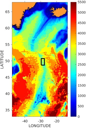
The model domain for the experiments presented here covers the North Atlantic between Greenland and the Iceland, from 48° W to 13° W and 33° to 67.92° N, with the Faraday Fracture Zone AOI indicated by the solid black box (Figure 1). Both the NR and the AR models use a spherical projection with a horizontal resolution of 2 km. The NR has higher vertical resolution with 100 levels in the vertical (45 sigma) extending to a maximum depth near 5500 m. The AR model, on the other hand, has lower vertical resolution (50 levels, 25 sigma). It was decided to configure the NR with higher vertical resolution relative to the AR, rather than with higher horizontal resolution. This is due to the possibility that in the deep water, in regions with strong tides where solitary-like internal waves are generated, higher horizontal resolution could result in internal waves that are too steep as they cannot break in a hydrostatic model (T. Jensen, personal communication, 7 May 2020).

Figure 1. North Atlantic Ocean domain used in the twin data assimilation experiment. Bathymetry shown in colour contours; Faraday Fracture Zone (the area of interest) shown by the black box in the centre of the domain.

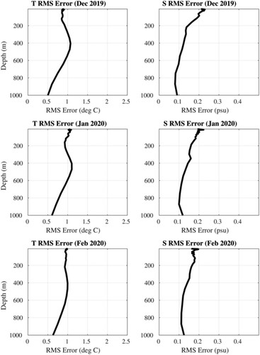
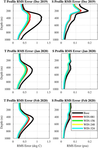
There are two primary experiment time frames presented here. The first experiment takes place from late June through August 2019. In this case the NR initial condition is derived from GOFS on 1 May 2019 and the model is run through 1 September 2019. The AR model initial condition is on 15 June 2019; this initial condition comes from an offset model state derived from the NR on 1 July 2019. This has the effect of displacing eddies and fronts in a manner that is consistent with realistic ocean model errors (relative to real observations). Figure 2 shows a four-panel plot of average profile RMSE between the NR and the AR model (prior to data assimilation) for temperature (left panels) and salinity (right panels) for the entire month of July (top panels) and August (bottom panels). These errors are consistent with the operational ocean model results for this domain when compared to real observations as employed by the Fleet Numerical Meteorology and Oceanography Command (FNMOC, not shown). The second experiment takes place from December 2019 through February 2020. In this case the NR initial condition is derived from GOFS on 1 October 2019 and run through February 2020. The AR model initial condition is on 15 November 2019 where the initial state comes from an offset model state derived from the NR on 1 December (in the same manner as the summer experiment). Figure 3 shows the same as Figure 2, but for the winter experiment. The character of the error in the winter is different than the summer (e.g. smaller error in the mixed layer, less variation of error in the vertical), but the error magnitude remains consistent (∼1°C). It should be noted that the twin data assimilation setup described here does not constitute a true OSSE as defined by Halliwell et al. (2014). Specifically, this configuration uses a NR that is of the same horizontal resolution as the AR and both the NR and AR use the same model, lateral and surface boundary conditions, and physical parameterizations. This is deemed acceptable for this work, however, as the statistical differences between the NR and the AR (non-data-assimilating) are of the same magnitude of error as the Navy’s operational ocean forecasting system (when compared to observations) as mentioned previously in this section.

Figure 2. Non-assimilative (free run) model average profile root-mean square error compared to the NR for July (top panels), August (bottom panels), temperature (left panels), and salinity (right panels).

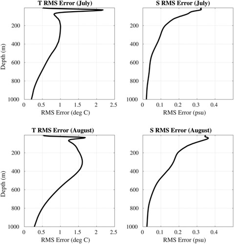
Figure 3. Same as Figure 2, but for the wintertime float deployment experiment (1 December 2019 through 29 February 2020).

2.2. The data assimilation algorithm and NR observation sampling strategies

The data assimilation algorithm used in this work is the NCODA-3DVAR system version 4.1. NCODA-3DVAR uses a second-order autoregressive function to model the background error correlation in both the horizontal and vertical. The horizontal error correlation length scales are based on the Rossby radius of deformation, whereas the vertical error correlation length scales are based on density gradients (with adjusted scales within the mixed layer). The background error variance is reduced in the vicinity of recently assimilated observations using the analysis error variance calculated by NCODA. These errors are grown over time, towards the climatological error variance, for regions that are not sampled by observations. NCODA v4.1 reduces the spatial density of observations in two different ways, depending on whether the observation is a surface observation or a vertical profile. For surface observations, such as sea surface temperature (SST) and sea surface height (SSH), NCODA produces ‘super-observations’ by averaging within a certain radius (typically defined by the background horizontal error correlation length scale). Profile observations, on the other hand, are reduced in number by removing observations that are too close in space to other profile locations (no averaging is done). The spatial radius that defines this ‘closeness’ can be adjusted with a user parameter. In the work done here, this parameter was set such that a maximum number of profile observations could be included in the data assimilation; this setting allowed for all profiles from each experiment to be included at the initial time.

Essentially two sets of observations are sampled from the NR to be assimilated by the AR model: standard observations and the special deployment of profiling floats. The standard observations include all those that would typically be available to the operational models on a daily basis. For this, the actual locations and types that were available for both experiment time frames (25 June through 1 September 2019 and 1 December 2019 through 29 February 2020) are used; the values are derived by interpolating the NR solution at the time of the observation to its location. This is straightforward for remote and in-situ observations of temperature and salinity. For SSH, however, some additional care was taken in order to properly mimic how these observations are treated by the operational system. Detided observations of along-track SSH anomaly (SSHA) are typically transformed into profiles of temperature and salinity by either the Modular Ocean Data Assimilation System (MODAS; Fox et al. 2002) or the Improved Synthetic Ocean Profiles (ISOP; Helber et al. 2013) system. For ISOP, this involves constructing a sub-surface temperature profile that has a prescribed mixed layer depth (typically from the background model), a dynamic layer that is constructed with covariances of SST and SSH with coupled empirical orthogonal functions (EOFs) of temperature and salinity, in addition to coupled EOFs of vertical gradients of temperature and salinity in the upper 1000 m. This dynamic layer is then merged with climatology to form the deeper layers. For this experiment, since tides are present, the model SSH solution will have a strong surface tide signal. To work around this issue, the steric height (SH) rather than the model SSH is sampled from the NR as a proxy for observed SSH. Steric height is computed directly from the model temperature and salinity by first computing the specific volume anomaly (SVA) and then integrating that to some specified depth: (1) $\begin{array}{rl}\mathrm{SVA}=& {\displaystyle \frac{{\rho }_o(T_o,S_o,p)-\rho (T,S,p)}{{\rho }_o(T_o,S_o,p)}}\\ \mathrm{SH}=& \underset{0}{\overset{z}{\int }}(\mathrm{SVA})\mathrm{d}z\end{array}$(1) where ρ_o is a reference density for salinity at 35 psu and temperature at 0°C. This is convenient since MODAS and ISOP both derive temperature and salinity synthetic profiles for the steric component of the SSH. Ultimately, steric height anomalies (SHA) are passed to MODAS or ISOP to generate synthetic temperature and salinity profiles that are assimilated into AR. In order to compute the SHA from SH, a long-term mean SH from the Generalised Digital Environmental Model (GDEM; Carnes 2009) climatology is removed.

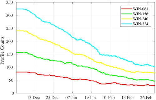
The in-situ profiling floats are sampled using a gridded deployment. The gridded network starts with an upper limit of deployable floats (as provided by FNMOC) as 324 floats for the first experiment. To determine what minimum number of floats is needed, this is decreased in increments to produce three additional experiments using 240, 156, and 81 floats, respectively. The initial deployment for each experiment is shown in Figure 4 and are known here as SUM/WIN-324 (summer and winter; far right panel), SUM/WIN-240 (inner right panel), SUM/WIN-156 (inner left panel), and SUM/WIN-081 (far left panel), with the AOI indicated by the inner box outline. These deployments provide differing horizontal data resolutions, roughly 12 km for 324; 15 km for 240; 18 km for 156; and 25 km for 81. In order to sample ocean profiles of temperature and salinity over time along the path of these simulated floats, a simple advection model was used that utilises the NR velocity at the float depth (1000 m) to advect the simulated floats over time. The floats are simulated to rise to the surface every two days at 0z; no horizontal advection is assumed to occur during the ascent and descent. This is not entirely realistic; however, this simplification is appropriate given the spatial scales of features resolved by the NR, the amount of horizontal displacement typically observed during real float ascent and descent, and the assumed background error correlation scales (which dictate the size of the correction derived from the float observations). Figure 5 shows the paths of each float over time (top panels) as well as the final positions of each float on 1 September 2019 from each deployment experiment (bottom panels) for 81 floats (far left panel), 156 floats (inner left panel), 240 floats (inner right panel), and 324 floats (far right panel). The influence of the Gulf Stream current can be seen as many of the floats are advected to the northeast of the AOI over time; however, many floats are pulled by smaller-scale eddies and other features to the north, south, and west over time. Not surprising, the experiment with the most initial deployments has the most floats within the AOI at the end of the experiment. Figure 6 shows the same as Figure 5, but for the deployment of floats in the winter months. Comparing Figures 5 and 6 it is apparent that the NR ocean velocities are stronger in the winter than the summer near the AOI, as the extent of the float movement is greater in the winter. Also, there are noticeably fewer floats at the end of the experiment in Figure 6 (bottom panels) than what is shown in Figure 5. We can examine the number of floats with the AOI over time. Figure 7 shows the total profile count inside the AOI from each deployment during the summer-time experiments with SUM-324 (cyan), SUM-240 (yellow), SUM-156 (green), and SUM-081 (red). Each deployment shows the greatest reduction of floats from about 26 July to nearly 1 September 2019. Figure 8 shows the same as Figure 7, but for the deployment of floats in the winter-time experiment. Comparing the deployments between the summer (Figure 7) and winter (Figure 8) shows that the AOI loses floats at a faster pace in the winter than the summer. For example, SUM-324 (Figure 7) has more than 300 floats remaining in the AOI after one month, whereas the same deployment in the winter (WIN-324, Figure 8) indicates that only about 250 floats remain in the AOI after one month. This will have significant consequences in terms of ocean model performance as will be shown later.

Figure 4. Profiling float deployments on 25 June 2019 (summertime) and 1 December 2019 (wintertime) sampling data from the NR for 81 floats (far left panel), 156 floats (inner left panel), 240 floats (inner right panel), and 324 floats (far right panel).

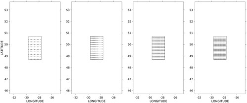
Figure 5. Profiling float trajectories (top panels) and final float positions (bottom panels) for the summertime float deployment (25 June through 1 September 2019) using 81 floats (far left panels), 156 floats (inner left panels), 240 floats (inner right panels), and 324 floats (far right panels).

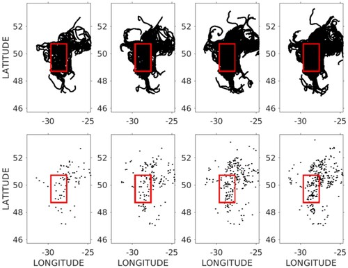
Figure 6. Same as Figure 5, but for the wintertime deployment (1 December 2019 through 29 February 2020).

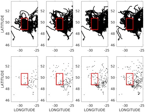
Figure 7. Total profiling float count within the AOI from each of the summertime float deployment experiments (25 June through 1 September 2019).

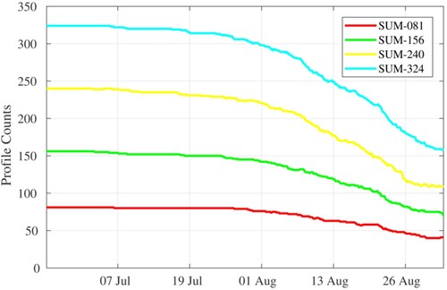
Figure 8. Same as Figure 7, but for each of the wintertime float deployment experiments (1 December 2019 through 29 February 2020).

2.3. Evaluation metrics (mixed layer and thermocline depth)

The derived quantities from the 24-hour forecast in the AR that are evaluated for this work are the mixed layer depth (MLD) and thermocline depth (TD). These are important quantities for ocean modelling for a number of reasons. For example, the MLD can play an important role in upper-ocean heat content and its impact on tropical cyclone development (Mao et al. 2000); for the TD, capturing the depth of the thermocline accurately can impact the proper magnitude, shape, and orientation of mesoscale eddies as anticyclonic (warm-core) eddies tend to deepen the thermocline whereas cyclonic (cold-core) eddies tend to exhibit shallower thermocline layers in the sub-surface (Chen et al. 2011). For ocean modelling, accurately representing these features can impact the model simulation of ocean circulation, heat content, and air–sea interactions. To that end, examining the impact (through assimilation) of various deployments of profiling floats on the forecast of these features is important.

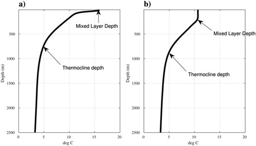
There are a number of methods to compute MLD, mainly focusing on the vertical temperature or density gradient from the ocean surface to some depth (Helber et al. 2013). For the work shown here, the algorithm that is embedded within NCODA is used. This method uses the temperature profile only and, starting from the ocean surface, simply searches for the vertical depth where the temperature difference from the surface temperature exceeds 0.5°C. For the TD, finding the vertical position where the temperature gradient approaches zero is rather difficult due to slight level-to-level variations in any given model temperature profile. Due to this, a representative proxy is used that generally describes the depth of the thermocline within the AOI. Figure 9 shows the average temperature profile within the AOI during the summer (Figure 9(a)) and winter (Figure 9(b)) experiments; the average MLD is also indicated on each profile in Figure 9 for reference. It is determined that the level of the 5.0°C isotherm provides an adequate approximate location of the TD. This is similar to approaches used in literature, as mentioned in Yang and Wang (2009), where, for example, the 20°C isotherm has historically been used as a proxy of the TD within the equatorial Pacific. In this AOI, during this experiment time frame, the 5°C isotherm is deemed appropriate. This level is computed for each model grid point within the AOI for both the winter and summer experiments and used to evaluate the TD from each model run relative to the NR. For each of the MLD and TD results shown in the next section, the 24-hour model forecast is compared directly to the NR fields for evaluation.

Figure 9. Average temperature profile within the AOI during the (a) summertime deployment and (b) wintertime deployment. Approximate location for the average MLD and TD is indicated.

3. Summer-time experiment results

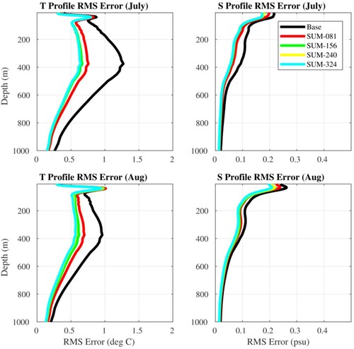
It is useful to examine the 24-hr forecast fields in terms of standard oceanographic variables, such as profile RMSE for temperature and salinity. Figure 10 shows this metric for the summer deployment experiments as well as an experiment known as ‘the Base Run’ for average profile RMSE in July (top panels) and August (bottom panels) in temperature (left panels) and salinity (right panels). The Base Run is intended to represent the typical data-assimilative forecast model for this basin. The assimilation for this experiment includes SST and SSH data, as well as any available sub-surface glider or ARGO observations that happen to be within the domain during the experiment time frame. Since the NR is sampled for standard observations using the actual observation locations collected during both the summer and winter time periods, there are some glider and ARGO sub-surface observations present within the larger model domain. These data are common between the Base Run as well as each of the SUM and WIN special float deployment experiments. In Figure 10 the AR model results from each experiment are compared directly to the NR, within the AOI, interpolated vertically due to the different vertical resolutions (NR 100 layers vs AR 50 layers). Two primary findings stand-out for temperature and are seen in both July and August results: (1) there is a substantial reduction of error over the Base Run in the deep water below 100 m when additional floats are assimilated, and (2) there is not much difference in error between the Base Run and the float deployment runs in the near surface (less than 50 m depth), around where the mixed layer is situated for this domain during the summer months. This is not the case for salinity, on the other hand, where improvement is seen from the surface down to at least 600 m depth, with the SUM-324 experiment showing the best results (though only slightly over SUM-240). In any case, these results indicate that the error near the average mixed layer depth in July and August is roughly identical between the Base Run and all of the float runs.

Figure 10. 24-hour model forecast profile RMSE averaged over each month (as compared to the NR within the AOI) between the Base Run (solid black line), and each of the summertime float deployment experiments (colour lines) for July (top panels) and August (bottom panels) in temperature (left panels) and salinity (right panels).

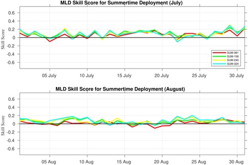
Figure 11 shows the time series of MLD RMSE in July (top panel) and August (bottom panel) for the Base Run and the four float deployment experiments. As expected, given the temperature error analysis shown in Figure 10, there is not much difference between the Base Run and the float deployment experiments in terms of MLD. When results are this similar it can be helpful to examine a skill score (SS) metric to accentuate any gained skill in one run relative to another. In this case, we can examine the RMSE of each of the float deployments relative to the RMSE in the Base Run in the following manner: (2) $\mathrm{SS}=1.0-{\displaystyle \frac{\mathrm{RM}{\mathrm{S}}_{\mathrm{floats}}}{\mathrm{RM}{\mathrm{S}}_{\mathrm{base}}}}$(2) where RMS_floats refers to the RMSE of one of the float deployment experiments. Here the SS metric is interpreted to say that values above 0.0 show skill gained in the float experiment relative to the Base Run; and values less than 0.0 show skill lost. Figure 12 shows the MLD SS metric for July (top panels) and August (bottom panels) for each float deployment experiment. Figure 12 shows slightly positive to negligible skill gain when deploying any number of floats in the AOI relative to the Base Run, which has no additional floats added. At times the skill is slightly positive, and other times it is slightly negative, but in both cases to a very small magnitude. This experiment suggests that for this area (Faraday Fracture Zone) and this time of year (northern summer months), the model representation of MLD is not strongly impacted by the number of profiling floats. This result suggests that another observation, common to both the Base Run and all of the float experiments, possibly has the dominant role in determining the model MLD forecast. We hypothesise that this observation is satellite sea surface temperature (SST).

Figure 11. Mixed Layer Depth (MLD) RMSE (as compared to the NR within the AOI) from 25 June through 1 September 2019 for the Base Run (solid black line), and each of the summertime float deployment experiments (colour lines).

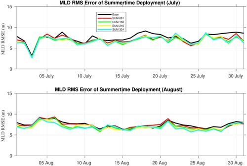
Figure 12. Mixed Layer Depth (MLD) skill score metric (relative to the Base Run) from 25 June through 1 September 2019 for each of the summertime float deployment experiments (colour lines).

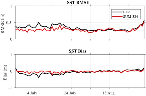
Figure 13 shows the surface distribution of assimilated super-observation SSTs for 1 July 2019 within the AOI. This distribution is common between all the float experiments as well as the Base Run, and is representative of each analysis day throughout the experiment. As can be seen, there is excellent coverage over the entire area from SST observations. Figure 14 shows the horizontal background error correlation scale used by NCODA-3DVAR in the AOI (left panel) and the vertical background error correlation scale at a point near the centre of the AOI (right panel). These correlations are responsible for spreading information from individual observation locations to the rest of the model domain during the data assimilation phase. The horizontal correlation scale is fixed in time and is based on the Rossby Radius of deformation, while the vertical correlation scale is based on a climatology-derived vertical density gradient (Cummings and Smedstad 2013). As such, the vertical correlation scale will vary by month over the course of the experiment, but not to a large degree. Given the observation distribution of SSTs seen in Figure 13, and the horizontal correlation scales shown in Figure 14 (between 20 and 30 km), it is clear that there is sufficient surface coverage of SST observations (essentially no gaps). The vertical correlation scale, as mentioned previously, is based on the density gradient with an adjustment for the mixed layer. This adjustment can be seen from 0 to 15 m depth where the correlation scale is relatively large near the surface (about 23 m) and reduces to about 15 m at 15 m depth. This has the effect of strongly projecting SST observation information into the ocean model interior relative to the shallow mixed layer present in the AOI during northern-hemisphere summer. This is desirable, of course, given the existence of the mixed layer, where the temperature should be relatively uniform to the base of the mixed layer. Therefore, if both the Base Run and the collective float experiments are constraining the model SST and temperature through the mixed layer to the same degree, primarily through the assimilation of SST observations, it would stand to reason that each experiment would be presenting roughly identical MLD throughout the AOI. Figure 15 shows the error in the 24-hr SST between the Base Run and the float deployment experiments. Here the model SST RMSE (top panel) and bias of the Base Run (black line) and experiment SUM-324 (red) relative to the NR within the AOI is shown from 25 June through 1 September. Figure 15 shows that the error in the Base Run and SUM-324, in regards to SST, is very similar, with some slight improvement shown in the SUM-324 experiment with the addition of float observations over the Base Run. Overall, however, this suggests that both experiments are constraining the upper-ocean temperature to roughly the same degree. Given this, it is not surprising that there is not much difference between the Base Run and the various float experiments. In each case we conjecture that the temperature representation of the upper 50 m of the model ocean (the average depth of the mixed layer during this time period) is primarily controlled by SST observations. It is possible that there is seasonality in this result. It is known that the MLD is relatively shallow in the summer months in this part of the Atlantic and deeper in the winter months. Given this, a deeper MLD may be more heavily impacted by sub-surface observations than a shallower MLD. This will be examined in the next section.

Figure 13. SST super-observation locations on 1 July 2019 (within the AOI).

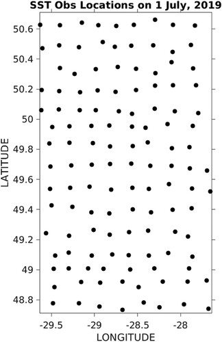
Figure 14. NCODA-3DVAR horizontal background error correlation scales within the AOI (left panel in kilometres) and the vertical background error correlation scale at a grid point near the centre of the AOI.

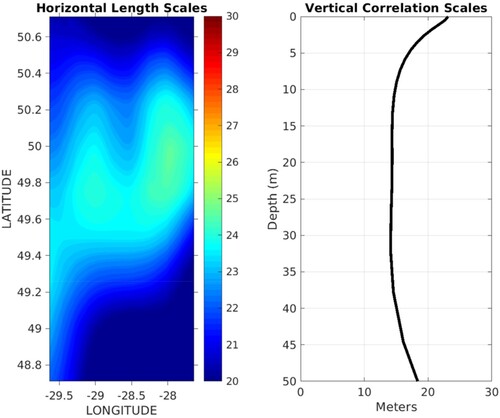
Figure 15. RMSE (top panel) and bias (bottom panel) in the ocean model SST for the Base Run (black line) and the summertime float deployment experiment with 324 floats (red line) as compared to the NR within the AOI from 25 June through 1 September 2019.

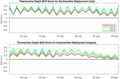
The profile temperature RMSE shown in Figure 10 shows substantial improvement in temperature below the average MLD. The error in TD should be more heavily impacted by profiling floats as the influence of SST observations in the deeper portion of the water column is much less. Figure 16 shows the TD RMS over time in July (top panels) and August (bottom panels) for the Base Run (black) and each float deployment. Here the additional float observations result in model simulations of TD that are better (at times greater than 100 m RMSE) than the Base Run. Examining these results more closely it should be noted that the experiments with 156, 240, and 324 floats perform remarkably similar for much of the experiment time frame. This suggests that there may not be much gained in deploying more than twice the number of floats, beyond 156, for this area during this time of year and using this data assimilation system and settings. This can be seen perhaps more clearly in Figure 17 that shows the SS metric for TD during July (top panels) and August (bottom panels) for the float deployment experiments. Here it is clear that each float experiment shows a gain of skill over the Base Run, but the experiment with the least number of floats (81) is the outlier. Roughly doubling the number from this experiment (156) results in a substantial increase in skill gained over the Base Run. Further increasing the number of floats results in much less gain in skill. It should be noted that there is a noticeable ‘saw-tooth’ pattern in the RMSE and skill score for each float experiment in Figures 16 and 17. This is due to the decrease in error brought by the assimilation of the special float deployment data and the subsequent rise in the AR error relative to the NR during the time this data is not available. This same pattern is not seen in the MLD error plots shown in Figures 11 and 12 due to the previously mentioned hypothesised dominance of the SST assimilation on the MLD representation during this summertime period.

Figure 16. Thermocline depth (TD) RMSE (as compared to the NR within the AOI) from 25 June through 1 September 2019 for the Base Run (solid black line), and each of the summertime float deployment experiments (colour lines).

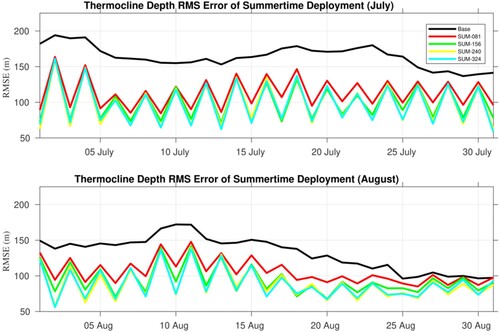
Figure 17. Thermocline (TD) skill score metric (relative to the Base Run) 25 June through 1 September 2019 for each of the summertime float deployment experiments (colour lines).

4. Winter-time experiment results

The deployment of simulated floats is done again in the FFZ AOI, but this time in the northern hemisphere winter months of December 2019 through February 2020. The preceding experiments indicated that in the summer the model MLD performance is dominated by the assimilation of SST observations, likely due to the relatively shallow ocean MLD during this time frame over the AOI. In the winter over the AOI, however, the MLD shows more variation and tends to be deeper. Before examining the model performance in terms of MLD and TD, though, it is important to once again examine the AR performance relative to the NR in terms of model temperature and salinity. Figure 18 shows the average profile RMS error for temperature (left panels) and salinity (right panels) for December 2019 (top panels), January 2020 (middle panels), and February 2020 (bottom panels), computed by comparing the AR and NR at each grid point within the AOI. Each float deployment experiment is shown (coloured lines), along with the Base Run (solid black). The character of the error in the model temperature is very different in the winter than the summer in the AOI. The summer (Figure 10) display two error maxima, one at the base of the average mixed layer (∼50 m) and another in the deep water between 200 and 400 m (near the mid-point of the average summertime thermocline layer as shown in Figure 9). The winter, on the other hand, has nearly constant error from the surface to 200 m depth, with a single error maximum between 400 and 600 m (again, near the mid-point of the average wintertime thermocline layer as shown in Figure 9). The large error in the Base Run within the thermocline is likely due to misplaced eddies and fronts relative to the NR. The addition of floats does seem to reduce the error in temperature during the wintertime experiment compared to the Base Run from 0 to 200 m depth, at least during the first month (Figure 18, top left panel); this is opposite of what is seen during the summertime experiment. This drop in error over the Base Run from 0 to 200 m depth is much smaller in January and February, likely due to the lack of floats remaining in the AOI (Figure 8). The addition of floats leads to a dramatic decrease in error in salinity during December (Figure 18, top right panel), but less improvement in January and December.

Figure 18. 24-hour model forecast profile RMSE averaged over each month (as compared to the NR within the AOI) between the Base Run (solid black line), and each of the wintertime float deployment experiments (colour lines; 1 December 2019 through 29 February 2020). Top panels show December 2019; middle panels show January 2020; bottom panels show February 2020.

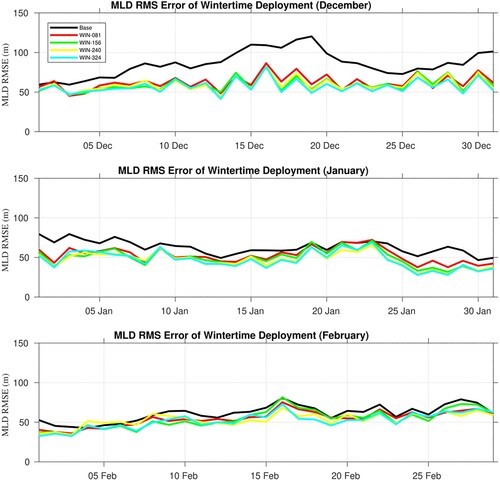
We can now examine the model performance in terms of the MLD. Figure 19 shows the time series of MLD RMS error for December 2019 (top panel), January 2020 (middle panel), and February 2020 (bottom panel) within the AOI for the Base Run (solid black) and each of the four float deployment experiments. Unlike the summer experiments, these results strongly indicate that the assimilation of additional float observations has a strong positive impact on the model MLD, reducing the error in MLD from that of the Base Run by as much as 50 m RMS error (a 50% reduction). Again, like the summer experiments, there is very little variation in the model MLD error between float deployment experiments as WIN-156 has roughly the same error as WIN-324; only WIN-081 tends to have, at times, markedly different error. The error magnitude of MLD is much higher during these winter months (> 50 m) over the AOI than the summer (∼10 m), likely due to the deeper MLD and greater spatial variation during this time frame (Helber et al. 2008). Figure 19 further indicates that the reduction in the total number of floats in the AOI over time has a dramatic negative impact on the model MLD performance, as the RMS error in the float experiments stays relatively flat in January (as the Base Run error drops), and increases in February to match that of the Base Run. This suggests that re-deployment of floats is required during the winter months in this area and should be done as often as needed given the ocean currents in the AOI.

Figure 19. Mixed Layer Depth (MLD) RMSE (as compared to the NR within the AOI) from 1 December 2019 through 29 February 2020 for the Base Run (solid black line) and each of the wintertime float deployment experiments (colour lines).

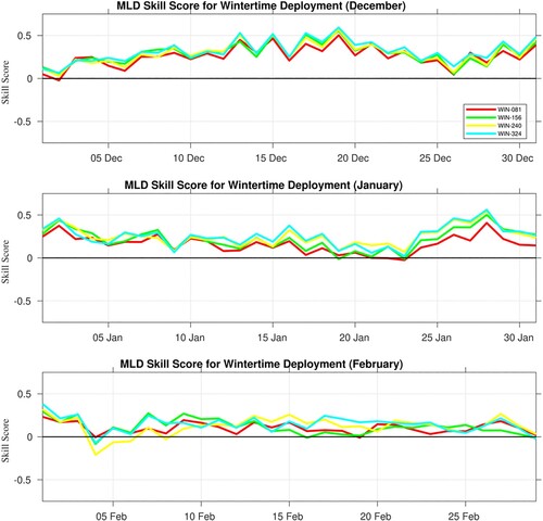
Figure 20 shows the MLD skill score of the float deployment experiments, relative to the Base Run for December 2019 (top panel), January 2020 (middle panel), and February 2020 (bottom panel). Again, unlike the summer experiments, these winter-time deployments produce strong skill gain over the Base Run during the first month to month and a half, as the skill score is near +0.5 during this time period. There is some gain in skill going from 81 to 156 floats, but like the summer experiments, there is not much gain in skill when increasing the float count from 156 to 240 or 324. It should be noted here that Figures 19 and 20 show some of the ‘saw-tooth’ error pattern shown in the thermocline depth error plots from the summertime deployment. It is noticeable here in the MLD results during the wintertime deployment due to the deeper MLD in this time frame and the increased impact of the special float deployment data on the resulting model analysis and forecast.

Figure 20. Mixed Layer Depth (MLD) skill score metric (relative to the Base Run) from 1 December 2019 through 29 February 2020 for each of the wintertime float deployment experiments (colour lines).

Figure 21 shows the time series of TD RMS error for December 2019 (top panel), January 2020 (middle panel), and February 2020 (bottom panel), for the Base Run (black line) and each of the float deployments (coloured lines). Like the summer months, the model performance in TD is strongly tied to the number of floats in the AOI, as each of the float deployments shows an improvement in RMS error over the Base Run for the first month and a half. Like the MLD results, though, the TD performance degrades relative to the Base Run as the number of floats in the AOI reduces over time. The relative error magnitude in TD is roughly the same in the winter as it is in the summer, indicating no seasonal dependence on model TD performance. Figure 22 shows the TD skill score for each of the float deployments relative to the Base Run for December 2019 (top panel), January 2020 (middle panel), and February 2020 (bottom panel). Each of the float experiments shows a good gain in skill relative to the Base Run until about mid-January when the performance becomes relatively identical to the Base Run, though there is some improvement in early February. Again, as earlier results indicated, there is some useful skill to be gained when assimilating 156 floats rather than just 81, but not much gain in skill when increasing beyond that number. Both Figures 21 and 22 exhibit the saw-tooth pattern as well for reasons previously mentioned.

Figure 21. Thermocline depth (TD) RMSE (as compared to the NR within the AOI) from 1 December 2019 through 29 February 2020 for the Base Run (solid black line) and each of the wintertime float deployment experiments (colour lines).

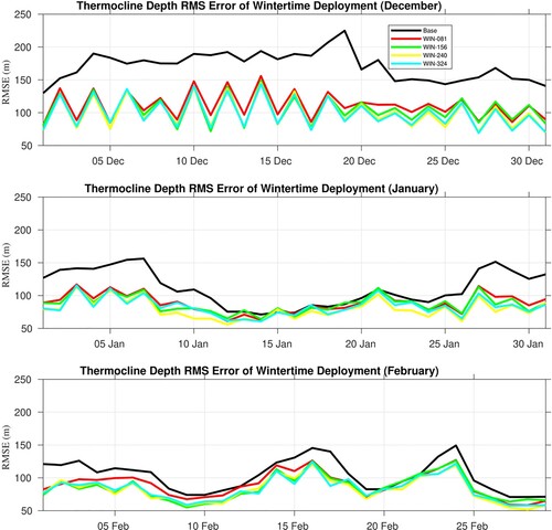
Figure 22. Thermocline depth (TD) skill score metric (relative to the Base Run) from 1 December 2019 through 29 February 2020 for each of the wintertime float deployment experiments (colour lines).

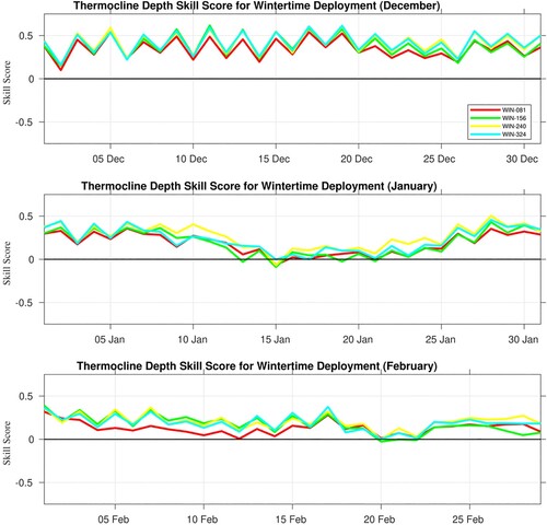
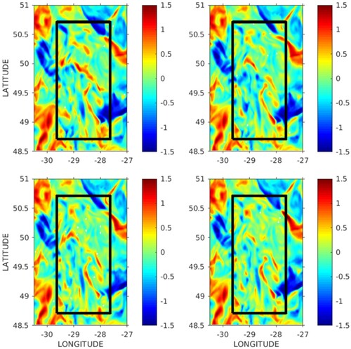
We further examine the results from Figures 19–22 to determine why there is not much skill gain in the model performance during December 2019 when increasing the number of assimilated floats from 81 to 324. As seen in Figure 20, there is some skill gain when increasing the number of floats from 81 to 156; however, there is not much improvement when increasing the number of floats further. To determine the possible cause of this, the field of innovations (model forecast -observation differences) and the increments from the data assimilation are examined. Figure 23 shows the innovations in temperature (coloured dots) overlaying the analysis increments (colour contours) at 100 m depth within the AOI on 1 December 2019 (the first analysis day of the winter experiment) for WIN-081 (upper left), WIN-156 (upper right), WIN-240 (lower left), and WIN-324 (lower right). The 100 m depth is used as a representative field to examine as it is far enough removed from the influence of SST observations, but still shallow enough to capture the influence of mesoscale eddies on the model and observations. Figure 23 shows that the NCODA-3DVAR performs well in capturing the observation information as the increment fields represent the innovations well (given assumed observation and background error variance). The spatial distribution of the increments differs between WIN-081 and WIN-156, as WIN-156 captures some small-scale features in the increments that are not apparent in WIN-081; this is not surprising, as WIN-156 has nearly twice the number of float observations available for assimilation. Interestingly, the spatial pattern of the increments does not change much from WIN-156 to WIN-240 and WIN-324. This is despite a substantial increase in observations and the fact that the higher float counts are capturing some features that are not well-represented in the increment fields (areas where the innovation ‘dots’ do not match the increments). We can examine the impact of these increments on the forecast by comparing the subsequent 24-hour forecast directly to the NR within the AOI. Figure 24 shows this comparison as the difference in 100 m temperature between the NR and WIN-081 (upper left), WIN-156 (upper right), WIN-240 (lower left), and WIN-324 (lower right). The character of the difference between the NR and each model run is that the difference is broader in terms of spatial scale and magnitude in the area immediately surrounding the AOI, however within the AOI the difference exhibits small spatial scale structure and lower magnitudes, obviously the effect of the assimilation of float data in the analysis 24-hrs prior. What is most interesting is that the character of this difference within the AOI does not change much between experiments WIN-156, WIN-240, and WIN-324, as it seems the analysis was capable of correcting errors only to a certain spatial scale. This spatial scale is the assumed background error covariance length scale used in the 3DVAR assimilation. Recall from Figure 14 that the background error correlation scale within the AOI ranges from 20 to 26 km. Initially, the WIN-156 experiment positions the floats approximately 18 km apart, whereas floats with WIN-240 (WIN-324) are roughly 14 km (11 km) apart. Given this information, it is likely that the impact of the additional floats past WIN-156 has little impact on the ocean model forecast due to the nature in which the 3DVAR assimilation is configured; WIN-240 and WIN-324 have floats that are too close together relative to the assumed background error correlation length scale. The 3DVAR, with these settings, is not capable of correcting errors in the model that are smaller than this assumed length scale. It is possible that a more sophisticated data assimilation approach, such as a multiscale 3DVAR (Souopgui et al. 2020) or 4DVAR (Ngodock and Carrier 2014), may be able to make better use of the spatially dense observations from WIN-240 and WIN-324. This will be investigated in a future study.

Figure 23. Model-observations innovations (colour dots) and analysis increments (colour contours) in temperature at 100 m depth on 1 December 2019 from each wintertime float deployment experiment: WIN-081 (upper left), WIN-156 (upper right), WIN-240 (lower left), and WIN-324 (lower right).

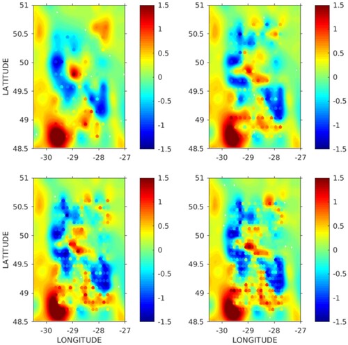
Figure 24. Temperature difference at 100 m depth between the NR and each wintertime float deployment experiment: WIN-081 (upper left), WIN-156 (upper right), WIN-240 (lower left), and WIN-324 (lower right). AOI outlined by black box.

5. Summary and future work

A twin data assimilation experiment is conducted here that aims to examine the impact of the spatial density of profiling floats on the ocean model 24-hr forecast of MLD and TD. A series of experiments are run, with varying numbers of profiling floats in northern hemisphere summer and winter deployments. The simulated float deployment used a fixed grid pattern over the area of interest (AOI, a 2° by 2° box covering the Faraday Fracture Zone). A second model run is done that assimilates only standard ocean observations and not the additional profiling float data. It is found that for this area and during the summer months (25 June through 1 September 2019), the ocean model MLD is most impacted by SST observations, and not the profiling floats. This is likely due to a combination of the relatively shallow MLD this time of year as well as the nature of the data assimilation algorithm (NCODA-3DVAR) that strongly projects SST corrections into the upper ocean via the vertical error covariance. When the TD is examined, on the other hand, the experiment with the most floats (324) tends to perform the best; however, the incremental improvement over using 156 floats is very small. The largest gain in skill is when the number of floats is increased from 81 to 156 floats. The winter-time experiments (1 December 2019 through 29 February 2020) show that the profiling floats have a greater impact on model MLD than during the summer months. This is likely due to not only the deeper MLD during these months but also due to the greater spatial variability of MLD during this time frame. As such, though the addition of floats provides an improved model MLD over the Base Run, the overall error in MLD is much higher (>50 m) than during the summer months (∼10 m). Also, the presence of stronger ocean currents during the winter months leads to greater float dispersion over time and to a more rapid reduction in float density in the AOI than during the summer months. This impacts the model’s ability to constrain the MLD one month after the float deployment and indicates the need for more frequent resampling of floats in this region during the winter months.

The fact that the 3DVAR data assimilation was not able to make better use of the higher float counts in WIN-240 and WIN-324 indicates a need for a more sophisticated data assimilation approach. A multiscale 3DVAR or 4DVAR may be able to make better use of the densely-deployed float observations and further reduce the error in MLD and TD beyond what is shown in this work. Another possibility is to continue to use the 3DVAR method, but to adjust the horizontal correlation scales to be shorter in the vicinity of fields of dense observations. This will be investigated in a follow-on study.

Disclosure statement

No potential conflict of interest was reported by the author(s).

Additional information

Funding

This work was supported by Fleet Numerical Meteorology and Oceanography Center and NRL paper contribution number NRL/JA/7320-22-5546.

Notes on contributors

Matthew J. Carrier

Dr. Matthew J. Carrier (PhD in meteorology in 2008 from The Florida State University) is an oceanographer with the U.S. Naval Research Laboratory and is an expert in data assimilation and numerical modeling.

Hans E. Ngodock

Dr. Hans E. Ngodock (PhD in applied mathematics and inverse modeling in 1996 from the Université Joseph Fourier) is an oceanographer with the U.S. Naval Research Laboratory and is an expert in data assimilation and numerical modeling.

Scott R. Smith

Dr. Scott R. Smith (PhD in Aerospace Engineering in 2002 from The University of Colorado) is an oceanographer with the U.S. Naval Research Laboratory and is an expert in numerical modeling, data assimilation, and tides.

Joseph M. D’Addezio

Dr. Joseph M. D’Addezio (PhD in oceanography in 2016 from the University of South Carolina) is an oceanographer with the U.S. Naval Research Laboratory and is an expert in ocean dynamics, modeling, and remote sensing.

John Osborne

Dr. John Osborne (PhD in physical oceanography and data assimilation in 2014 from Oregon State University) is an oceanographer with the U.S. Naval Research Laboratory and is an expert in numerical modeling, data assimilation, and ocean acoustics.

References

- Barron CN, Birol Kara A, Martin PJ, Rhodes RC, Smedstad L. 2006. Formulation, implementation and examination of vertical coordinate choices in the Global Navy Coastal Ocean Model (NCOM). Ocean Model. 11:347–375.
- Bleck R. 2002. An oceanic general circulation model framed in hybrid isopycnic-Cartesian coordinates. Ocean Model. 4:55–88. doi:10.1016/S1463-5003(01)00012-9.
- Carnes MR. 2009. Description and evaluation of GDEM-V 3.0. NRL Rep. NRL/MR/7330—09-9165, 24 pp. Available from: NRL, Code 7330, Bldg. 1009, Stennis Space Ctr., MS 39529-5004.
- Chen G, Hou Y, Chu X. 2011. Mesoscale eddies in the South China Sea: mean properties, spatiotemporal variability, and impact on thermohaline structure. J Geophys Res. 116:C06018. doi:10.1029/2010JC006716.
- Cummings JA, Smedstad OM. 2013. Variational data analysis for the global ocean. In: Park SK, Xu L, editors. Data assimilation for atmospheric, oceanic and hydrologic applications. Vol. II. Berlin Heidelberg: Springer-Verlag; p. 302–344. doi:10.1007/978-3-642-35088-7_13.
- Fox DN, Teague WJ, Barron CN, Carnes MR, Lee CM. 2002. The modular ocean data assimilation system (MODAS). J Atmos Ocean Technol. 19:240–252.
- Halliwell GR, Srinivasan A, Kourafalou VH, Yang H, Willey D, Henaff ML, Atlas R. 2014. Rigorous evaluation of a fraternal twin ocean OSSE system for the Open Gulf of Mexico. J Atmos Ocean Technol. 31:105–130. doi:10.1175/JTECH-D-13-00011.1.
- Helber RW, Barron CN, Carnes MR, Zingarelli RA. 2008. Evaluating the sonic layer depth relative to the mixed layer depth. J Geophys Res. 113:C07033. pp. 1–14. doi:10.1029/2007JC004595.
- Helber RW, Townsend TL, Barron CN, Dastugue JM, Carnes MR. 2013. Validation test report for the Improved Synthetic Ocean Profile (ISOP) System, Part I: synthetic profile methods and algorithm. NRL Rep. NRL/MR/7320—13-9364, 128 pp. Available from: NRL, Code 7320, Bldg. 1009, Stennis Space Ctr., MS 39529-5004.
- Hodur RM. 1997. The naval research laboratory’s coupled ocean/atmosphere mesoscale prediction system (COAMPS). Mon Weather Rev. 125:1414–1430. doi:10.1175/1520-0493(1997)125<1414:TNRLSC>2.0.CO;2.
- Kantha LH, Clayson CA. 2004. On the effect of surface gravity waves on mixing in the oceanic mixed layer. Ocean Modelling. 6:101–124.
- Mao Q, Chang SW, Pfeffer RL. 2000. Influence of large-scale initial oceanic mixed layer depth on tropical cyclones. Mon Weather Rev. 128:4058–4070. doi:10.1175/1520-0493(2000)129<4058:IOLSIO>2.0.CO;2.
- Ngodock HE, Carrier MJ. 2014. A 4DVAR system for the navy coastal ocean model. Part I: system description and assimilation of synthetic observations in monterey Bay. Mon Weather Rev. 142:2085–2107. doi:10.1175/MWR-D-13-00221.1.
- Souopgui I, D’Addezio JM, Rowley CD, Smith SR, Jacobs GA, Helber RW, Yaremchuk M, Osborne JJ. 2020. Multi-scale assimilation of simulated SWOT observations. Ocean Modelling. 154:101683. doi:10.1016/j.ocemod.2020.101683.
- Yang H, Wang F. 2009. Revisiting the thermocline depth in the equatorial pacific. J Clim. 22:3856–3863. doi:10.1175/2009JCLI2836.1.
- Zeng X, Atlas R, Birk RJ, Carr FH, Carrier MJ, Cucurull L, Hooke WH, Kalnay E, Murtugudde R, Posselt DJ, et al. 2020. Use of observing system simulation experiments in the United States. Bull Am Meteorol Soc. 101(8):E1427–E1438. doi:10.1175/BAMS-D-19-0155.1.