Calibration and validation of high frequency coastal radar waves exploiting in-situ observations and modelled data in the south-west Sicily

ABSTRACT

This paper describes a calibration procedure for a non-optimally configured High Frequency Radar (HFR) for the period 1 April 2021, to 31 March 2022, to assess sea waves characteristics. The HFR system, a 16.5 MHz WEllen RAdar (WERA), is part of an innovative network for monitoring the state of the sea. The system is installed in the western part of Sicily (Italy) where a wave buoy is positioned. HFR data underestimate the spectral significant wave heights (Hm0), in particular for Hm0 > 2 m, highlighting the need for calibration of the HFR system to ensure its optimal performance for operational purposes. The calibration was performed with both in-situ and modelled data provided by the Copernicus Marine Service. The best results were obtained when the buoy data were used as reference. Encouraging results were achieved as demonstrated by the improvement of the quantitative metrics after the calibration. Indeed, the RMSE decreased from 0.60 to 0.36 m; the correlation R increased slightly from 0.86 to 0.88, the slope from 0.48 to 0.8; whereas intercept from 0.11 to 0.31 m. Moreover, waves higher than > 2 m are well reproduced by the calibrated HFR time series with the RMSE decreasing from 1.3 to 0.53 m.

KEYWORDS:

• High frequency radar (HFR)
• wave buoy
• copernicus marine service (CMS)
• significant wave height
• calibration
• Sicily channel
• Mediterranean sea

1. Introduction

The accurate monitoring and forecasting of the sea state are essential for managing many activities (e.g. navigation, fishing, gas and oil extraction, offshore renewable energy installations, sports and recreation, etc.) and for increasing their safety. Multi-platform observing networks are crucial for wise coastal management (Pollard et al. 2019), sound design of infrastructures and the implementation of mitigation plans for extreme metocean hazards (i.e, storm surge floodings). Monitoring oceanographic parameters related to the dynamics of ocean surface waters, such as wave height and sea surface currents over time, as well as studying variations in temperature, sea level, and ocean circulation, are necessary because they allow us to observe and study how fast the climate is changing, especially in the context of global warming (Tintoré et al. 2019; Copernicus, 2022).

Marine technologies have greatly evolved, both through the use of in-situ fixed or mobile sensors, and remote sensing systems (Ardhuin et al. 2019; Lin and Yang 2020). Fixed systems typically consist of moored buoys with pressure, sound, and motion sensors capable of determining wave parameters, such as significant wave height, peak wave period and average wave direction during the peak wave period. The mobile in-situ systems typically consist of free buoys, such as drifters, which may be equipped with the same sensors as the fixed systems. Other examples of in-situ measurements are surveys conducted aboard research vessels or ships of opportunity. Remote sensing systems, on the other hand, are all based on the propagation of electromagnetic waves along the saline and well conducting ocean surface and relying on the analysis of the backscattered intensity and Doppler effects of radar signals. These radars are typically ground-based, but can also be installed at sea, in the air, and even on satellites (Izquierdo et al. 2004; Novi et al. 2020; Sun et al. 2020; Aouf et al. 2021). Lorente et al. (2022) describe in detail the ground-based HFR systems and show that they provide an impressive capability for monitoring large coastal areas, for a wide range of practical applications such as research, hazard management, maritime safety and rescue and vessel tracking (Reyes et al. 2022).

However, the use of in-situ acquisition systems and the use of remote sensing systems, often have different purposes and objectives related to their operational characteristics and thus can sometimes be considered as alternative and sometimes as complements. The use of remote sensing increases the amount of observational data available to fill the gaps associated with fixed monitoring systems and extends observation at a large spatial scale (Ardhuin et al. 2019; Rossi et al. 2021). Nevertheless, despite the technological advances, both systems have some critical issues. In particular, for buoys, the limits of continuous and correct data acquisition are often due to external factors related to the extreme environment in which they operate, such as unmooring, biofouling, collision phenomena with vessels or fishing gears, vandalism, maintenance difficulties and costs, sensors calibration, communication problems, and more (Ardhuin et al. 2019; Campos et al. 2021; Jensen et al. 2021; Ferla et al. 2022). All these problems may be the basis of the lack of data transmission, and in addition, the intervention times are never certain due to changing sea conditions. On the contrary, HFR is a land-based cost-effective technology that presents some additional advantages such as improved areal coverage; also HFR can effectively monitor sea states in densely operated maritime areas where fixed in-situ moorings may be compromised (such as in congested harbours). In the Mediterranean Sea there are several examples of studies with the use of radars and other systems both for data validation (Orasi et al. 2018; Saviano et al. 2019) and comparison with model data (Saviano et al. 2020) and last but not least for monitoring the state of the sea in different conditions (Lorente et al. 2021). However, the HFR band can be also affected by electromagnetic interferences or negatively impacted with the presence of metal items of orographic obstacles. They also require a lot of attention both because of their proximity to the marine environment and because of their complexity, since several systems must be installed in different and suitable positions to cover a given area. HFR technology is well developed and numerous systems of various types are available on the market (see Lorente et al. 2022 and references therein). Generally, HFRs are mainly optimised for detecting flow fields and they are often not entirely suitable for measuring wave data and are less reliable compared to in-situ wave measurement devices. Coastal HFR can be both direction-finding (for instance Coastal Ocean Dynamics Applications Radar, CODAR HFR, Barrick et al. 1985) and beamforming (for instance, WERA HFR, Gurkel et al. 1999). The former has the advantage of requiring a very limited area, since transmitting and receiving antennas are located in a single long-mast element. Despite the advantage of providing the wave-direction even with one single HFR site, measured direction and significant wave heights are not pointly but are referred to as concentric annular rings. The latter require: (i) a number of transmit antennas (usually four antennas arranged at the vertices of a square); (ii) a number of receive antennas (at least 8–16) arranged as a linear array.

Measurements of wave parameters such as spectral significant wave height, wave direction and spectral information require higher hardware characteristics than those expected for marine current measurement systems (Wyatt et al. 2011). The WERA HFR presents the advantage of providing wave parameters at each point over a predefined regular grid. However, systems with at least 12 antennas are needed when spatial variability in the wave field is fundamental and coverage over large areas in the ocean is required (Gomez et al. 2015). Nevertheless, the use of HFR with a smaller number of antennas is possible, with special precautions, to measure waves. In addition, the wave information is obtained from the peak values of the second-order spectra (Tian et al. 2020), which have a lower signal to noise ratio than the first-order return used for currents. This means that a smaller range is covered and also that the integration time should be longer than for currents (Gomez et al. 2015).

The products derived from these techniques, including those of the Copernicus Marine Service (CMS), can make an important contribution by covering large areas of our planet, albeit at lower spatial and temporal resolution (le Traon et al. 2017, 2019). CMS requirements for further development of the in-situ component of Copernicus include high priorities such as improving key observing systems such as ferry-boxes, gliders, tide gauges, and HFRs. Therefore, it is imperative to maintain and increase the number of wave buoys and incorporate wave measurements from HFR. Since April 2017, the CMS has been able to monitor wave height records during adverse weather conditions using two complementary data sources (i.e. wave models and in-situ platforms). In any case, these data must be integrated with those collected (buoy, radar HF, etc.) in order to calibrate and validate them and to compensate for the uncertainties of satellite data in coastal areas and shallow waters. Models must be considered an alternative in the absence of buoys or other systems, which often fail, especially nearshore.

In this paper, we present the preliminary results of a comparison between wave measurements collected and processed by three different systems in the period April 2021 to March 2022: an in-situ buoy, an HFR and the CMS numerical model in the area of the Sicily Channel (Mediterranean Sea, Figure 1). A method to calibrate HFR data is also presented with the aim of obtaining more reliable wave measurements, in order also to fulfil the request of CMS in-situ data. Studied area is presented in section2, section3 describes the datasets and section4 the theory. In section5 the results are presented and discussion and conclusions are given in section6 and 7, respectively.

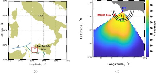
Figure 1. (a) Map of the area with the main circulation features: Atlantic current (AC), Atlantic Ionian Stream (AIS) and Tunisian Atlantic Current (ATC). The red rectangle indicates the studied area enlarged in (b), where the percentage of HFR data coverage from 1/4/21–31/031/22 is depicted. Mazara del Vallo ondametric buoy (red triangle) and WERA HFR position (blue triangle) are indicated. The area in green encloses the HFR grid points (blue points) considered in the analysis; the sector delimited by red lines corresponds to sFOV.

2. Study area

Our observations and study focus on the area off Capo Granitola, in southwestern Sicily, which corresponds to the northern part of the Sicily Channel (Figure 1). The Sicily Channel is generally considered as a corridor between the eastern and western Mediterranean Sea, where fishing, recreational activities and the transport of all kinds of goods, including dangerous ones, are very intense. This area is influenced by a series of complex oceanographic processes that distinguish it from the rest of the Mediterranean Sea (Bonanno et al. 2014). At the mesoscale, it is influenced by the dynamics of the lower atmosphere, especially wind stress, topography and internal processes, and therefore we can observe the presence of currents, jets, branches and eddies, which then have effects at a larger scale (Lermusiaux and Robinson 2001; Reyes Suarez et al. 2019).

The thermohaline circulation that affects the area is due to the inflow of less saline Atlantic water from the Strait of Gibraltar flowing eastward at the surface, and an intermediate layer of more saline Levantine water spreading westward and originating in the easternmost areas of the basin (Sorgente et al. 2011).

The Atlantic water, in the area off Capo Granitola, is composed of two different water currents that cross it: the Tunisian Atlantic Current (Sammari et al. 1999) located in the south near the African coasts and the Atlantic Ionian Stream, present in the north, near the Sicilian coasts (Robinson et al. 1999). The Atlantic Ionian Stream present in the study area and flowing eastward, can drive and modulate coastal upwelling. Its presence and evolution are variable in time and space, taking different more or less intense forms (Robinson et al. 1999; Sorgente et al. 2011; Basilone et al. 2013; Bonanno et al. 2013).

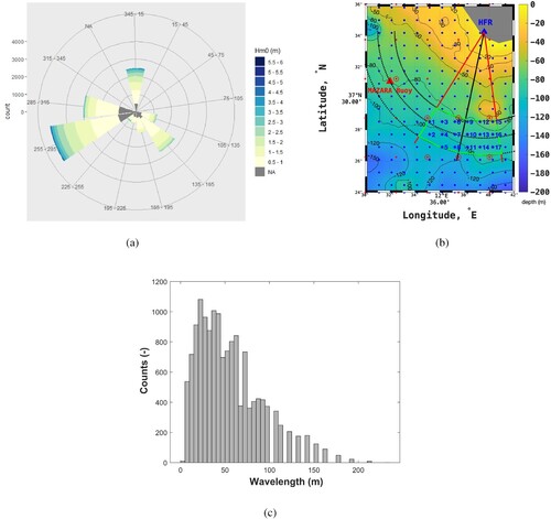
Hence, the study area is characterised by a directional distribution of spectral significant wave heights showing bimodal behaviour with two main incoming wave propagation sectors: the first from SE and the second from W (Figure 2a). This behaviour is well known in the area as bimodality of wave spectra and occurs frequently in medium energy swells but rarely during storms (Orasi et al. 2018).

Figure 2. (a) Directional distribution of significant wave heights measured by ondametric buoy. (b) Studied area with model grid points (red), radar grid points (blue) and superimposed bathymetry (from EMODNET, https://www.emodnet-bathymetry.eu/). The area in green contains the HFR points (blue stars numbered) where data have been considered for the comparison with buoy timeseries and for the correlation calculations with model points (red circles). Sector delimited by red lines corresponds to sFOV. (c) distribution of wavelengths λ measured from Mazara del Vallo Buoy (red triangle) in the period April 2021 - March 2022.

3. Materials

The coastal HFR used in Capo Granitola is a beamforming WERA system (Helzel Messtechnik GmbH) operating at a central frequency of 16.15 MHz. The system consists of 4 transmitting antennas and 8 receiving antennas which are the minimum number of receivers to obtain wave data, therefore the configuration is not optimal for wave monitoring (Gomez et al. 2015). The system can retrieve wave data with 1.5 km horizontal grid resolution and a sampling time of 15 min. Since only one radar site is available, only spectral significant wave height (Hm0_HFR) can be measured; while no wave direction information can be retrieved. At the operating frequency, the lower limit for Hm0_HFR, referred to as the noise threshold, is about 0.45 m, while the saturation limit corresponds to waves of 8 m (Wyatt 2002; Wyatt et al. 2011)

In-situ wave data are collected from the buoy located at Mazara Del Vallo (WMO code 61208); this buoy is part of the National Wave Network (RON), managed by ISPRA (National Research Institute for the Environment Protection), and it is moored at 37° 31’ 05’N and 12° 32’ 00’E at a sea depth of 85 m (Figure 1). RON data are freely available in Linked Open Data format (http://dati.isprambienteit). Spectral significant wave height data, hereafter referred to as Hm0_buoy were selected. Hm0_buoy ranged from 0.1–5.2 m during the studied period. Wave heights lower than 0.5 are considered calm sea states. Hm0_HFR data with WERA-default quality flag equal to 5 ( = bad) are removed.

In addition to wave heights measured by the in-situ buoy, wave data from a numerical model were provided by the CMS. As the interim reanalysis product is not available for the selected period, the analysis and forecast nominal product MEDSEA_ANALYSISFORECAST_WAV_006_017 is used. This is the nominal wave product of the Mediterranean Sea Forecasting system, composed by hourly wave parameters at 1/24° horizontal resolution covering the Mediterranean Sea (for the details https://resources.marine.copernicus.eu/product-detail/MEDSEA_ANALYSISFORECAST_WAV_006_017/INFORMATION). In particular, the dataset ‘med-hcmr-wav-an-fc-h’ is used and the extracted variable is the spectral significant wave height (VHM0) hereafter referred to as Hm0_CMS.

The analysis is carried out using a dataset collected during a 12-months (April, 1, 2021 to March, 31, 2022) period which starts contextually to the availability of buoy data (deployed in late March, 2021).

4. Methodology

The three data sources used in this study are characterised by different temporal and spatial resolutions. Regarding the temporal resolution, only the concurrent measures are used in the following calibration/validation steps. For the spatial resolutions, the grids for Hm0_CMS and Hm0_HFR are shown in Figure 2(b), but some consideration should be done before performing the calibration/validation. Although the Hm0_HFR measured by the WERA HFR system are in principle organised in a regular grid (finer than the CMS data), only the data over a subrange area are characterised by sufficient accuracies because the non-optimal HFR setup for wave measurements which requires the installation of 12 or 16 receiving antennas; for this reason the radar field has been restricted to eliminate the interference of the first-order lateral spectral peaks with the second-order spectral peaks from which the waves are calculated. Therefore, a sub-field of view (sFOV) is considered by restricting the full FOV as described in section 4.1. Once the HFR comparison area is established, because the in-situ buoy is located outside of the HFR comparison area (as well as it is outside of the entire HFR domain) it is mandatory to limit the comparison of wave data to the HFR grid points for which the deep water dispersion relation applies; under this condition and for short distances (a few tens of kilometres) the wave spectrum at the buoy site is comparable to that measurable at the HFR grid points.

The first step is to verify that the buoy measurements are representative of the wave state in the HFR comparison area. For this purpose, a comparison between Hm0_buoy and Hm0_CMS is performed at those model grid points closer to the HFR comparison area and buoy location.

Finally, the comparison between the uncalibrated significant wave heights Hm0_HFR,unc and Hm0_buoy is calculated for each grid point within the HFR comparison area at the same time to select the HFR reference point for the calibration.

4.1. WERA HFR calibration through means of Hm0Buoy and Hm0CMS data

The method used by WERA to estimate significant wave-height is an empirical method developed by Gurgel et al. (2006). The method assumes that there is a linear relationship between the WERA second-order backscatter spectrum (normalised by the first-order peak) and the wave energy spectrum multiplied by an angular spreading function. Since the second-order spectrum is folded around each of the Bragg peaks, the second-order backscatter energy, E_k, is calculated as the average of the spectral values on either side of the most energetic Bragg peak. This calculation is repeated for all Doppler-frequencies at intervals of 0.01 Hz, in the Doppler range from 0.05–0.25 Hz from the Bragg peak. In this way, the linear relationship contains 21 alpha coefficients (α_k) obtained from a field experiment (EuroROSE, Fedje experiment) with a 27.65 MHz HFR and a buoy (Gurgel et al. 2006). Given the normalised second-order power spectrum, E_k, measured by the HFR, the estimate of the wave energy spectrum, S_k, at each of the k-frequency considered is given by: (1) $S_K=E_K\cdot {\alpha }_{k@\mathrm{fradar}}$(1) where α_k@fradar are the alpha coefficients matched to the radar operating frequency (f_radar), as follows: (2) ${\alpha }_{k@\mathrm{fradar}}={\left({\displaystyle \frac{f_{@\mathrm{used}}}{f_{\mathrm{radar}}}}\right)}^2\cdot {\alpha }_{k@\mathrm{used}}$(2)

Finally, the spectral significant wave height (calculated from the spectral analysis) is determined considering the 21 wave energy spectrum S_k of the second order peak, i.e. using: (3) $\mathrm{Hm}0=4\sqrt{\sum _{k=1}^{21}0.01\cdot S_k}=0.4\sqrt{\sum _{k=1}^{21}{S}_k}$(3) where 0.01 is the frequency step in Hz.

By default, the set of α_k coefficients obtained from that field experiment with a 27.65 MHz HFR is used by the WERA station management software. Thus, only uncalibrated significant wave heights, Hm0_HFR,unc, are estimated after the installation of a WERA system.

To maximise the accuracy of the HFR wave height estimates, evaluation of a tailored set of α_k coefficients is mandatory. This calibration phase requires the use of an independent dataset of the wave energy spectrum S_k. However, if this is not available, the coefficients can be obtained from the significant wave height Hm0 obtained from a directional buoy or a reliable wave model, by least squares fit. Substituting equations (1) and (2) into equation (3) yields the following equation: (4) $\sum _{k=1}^{21}{E}_{\mathrm{kn}}\cdot {\alpha }_{k@\mathrm{used}}=6.25\cdot {\left({\displaystyle \frac{\mathrm{Hn}\cdot f_{\mathrm{rada}{r}_n}}{f_{@\mathrm{used}}}}\right)}^2$(4) which is in compact form of the type Eα = C, where E is the Nx21 matrix containing E_kn, C is the Nx1 vector formed by the right-hand side of equation (4), and N is the total number of measurements used. It can be solved for α using Hm0_n from a reference (buoy or model) by a least square fit, minimising the errors (C-Eα)². The least square fit is evaluated imposing a constraint on the α behaviour to obtain reliable values for α (Gomez 2019). In particular, the constraint matrix imposes some conditions on the evolution of α with frequency, i.e. on positive values and on first and second derivatives of the curve.

In this study, both the Hm0_buoy and Hm0_CMS values are used as independent reference datasets.

The α-values obtained with the above mentioned method, should then be tested and validated on a different period. For this reason, half of the available data are taken into account for the calibration/optimisation, whereas the validation process involves the remaining data. Thus, the available data set is splitted into the following time series: (i) from 1 April, to 31 July 2021 (D1); (ii) from 24 September 2021 to 31 March 2022 (D2).

The calibration is performed by taking into account Hm0_HFR data collected at the reference point defined by the preliminary analyses described in section 5.1.

5. Results

5.1. Results with uncalibrated HFR data

The sFOV is obtained by restricting the full FOV to the sector bounded by the delta angles equal to +20°/−20° with respect to the main antenna lobe bearing. Finally, the HFR comparison area is obtained by intersecting the sFOV with the annular ring of a thickness of D = 2 km, centred at the HFR-buoy distance (Figure 1b). The HFR comparison area contains 17 HFR grid points (blue stars in Figure 2b). The comparison between Hm0_buoy and Hm0_CMS, at the points closer to the selected area and at the buoy, reveals that Hm0_buoy and Hm0_CMS are comparable for all grid points with correlation values always above 0.96, at the 95% confidence level (hereinafter referred as ‘c.l.’). In addition, the comparison in terms of spectral significant wave height-distribution (summary statistics, validation metrics and qq-plots, not shown here) demonstrates that the series at the different points are in very good agreement. This result agrees with the deep water hydrodynamic condition which is verified at the buoy position and for several model points close to the HFR comparison area; however, small differences in correlation could be probably due to small changes of the wind input. The choice of the HFR grid-point among the ones in the green area, depends on the validity of the deep water dispersion law, and thus, on the wavelengths of the waves in the area.

The wave motion in the area during the considered period presents wavelengths (λ) mainly below 100 m (Figure 2c). Moreover, there is a consistent number of waves with λ between 70 and 100 m for which a bathymetry of 40–50 m is in disagreement with the dispersion law for deep waters (Dean and Dalrymple 1991). In particular, the bathymetry in the green area (Figure 2b) is always greater than 80 m, apart from the right-upper corner, characterised by a bathymetry of ∼40–50 m. Thus, according to these considerations, only points 12 and 15 are excluded from further analyses.

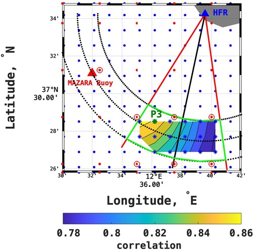
Regarding the Hm0_HFR,unc vs Hm0_buoy relationship, the points with the highest correlation coefficient are points 1 and 3 (Figure 3) with a correlation value of 0.86 at 95% c.l. Because point 1 is located too close to the western limit of the sFOV, beyond which the reliability of HFR wave data could be decreased, point 3 is selected as the best candidate point for the optimisation and validation calculations.

Figure 3. Correlation coefficient between Hm0_HFR,unc at stars within the green-bordered area and Hm0_buoy. Green star corresponds to the location P3 where HFR data have been considered for optimisation and validation.

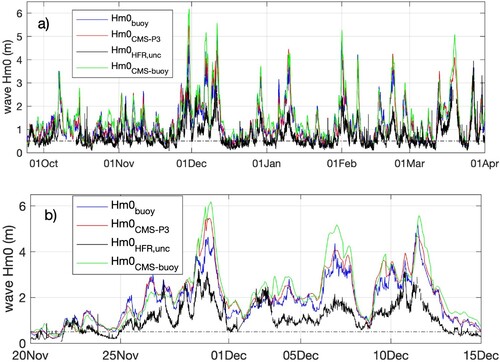
The time series comparison of Hm0_HFR,unc, Hm0_buoy and Hm0_CMS both at the buoy location (Hm0_CMS-buoy) and close to the point P3 (Hm0_CMS-P3), shown in Figure 4(a), reveals that the model captures well the peaks of wave height, although a light overestimation can also be observed. On the other hand, uncalibrated HFR data appears to underestimate, to some extent, mainly the main peaks, as for example the ones detected during the end of November-beginning of December 2021 or beginning of January 2022 (Figure 4b) or February 2022 (Figure 4c).

Figure 4. (a) Time series of Hm0_HFR,unc, Hm0_buoy, Hm0_CMS-buoy, Hm0_CMS-P3, obtained: from buoy (blue line), from HFR at P3 (black line) and from model data both at buoy location (green line) and close to P3 (red line). (b) zoom of (a) for the period 20/11/21–15/12/21. (c) zoom of (a) for the period 1/02/22–28/02/22. The dashed line indicates the noise threshold.

Although an underestimation of Hm0 measured by the HFR is clearly shown in the Hm0_buoy vs Hm0_HFR,UNC scatter plot (Figure 5a), most of the points of the dispersion appear well aligned as expected by looking at the high correlation value (Table 1). This underestimation could be a problem when using HFR data for operational purposes and thus, the calibration of the time series is mandatory. The possibility to calibrate the HFR measurements with the buoy data is confirmed by the high correlation (Table 1) shown also by the Hm0_buoy vs Hm0_CMS-P3 scatter plot, whose cloud appears well aligned to the 1:1 line (slope = 1.03, intercept = 0.01 m). Moreover, the very strong correlation of the Hm0_CMS-P3 vs Hm0_CMS-buoy confirms that the wave height spectrum at these two locations are quite similar (Table 1). Regarding the selection of the calibrating and validating periods to proceed with the calculation of the optimised alpha coefficients, it is chosen to use the second part of the data set (D2) for optimisation aims and the first part (D1) for validation. Indeed, it is preferable to use the autumn-winter period as the spectral significant wave heights span over a wider range.

Figure 5. Scatter plot of: (a) Hm0_HFR,unc at P3 versus Hm0 from buoy, and (b) Hm0 from model at P3 versus Hm0 from buoy for the period 1/4/2021–31/3/2022. Linear fit coefficients are indicated.

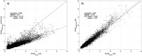
Table 1. Correlations (R), RMSE and bias among all timeseries at 95% confidence level for the period 1/4/2021–31/3/2022.

	Hm0CMS-P3	Hm0CMS-buoy	Hm0 buoy	Hm0HFR,unc
Hm0CMS-P3	-
Hm0CMS-buoy	R = 0.96 RMSE = 0.25 m bias = 0.08 m	-
Hm0buoy	R = 0.97 RMSE = 0.20 m bias = −0.04 m	R = 0.93 RMSE = 0.32 m bias = −0.11 m	-
Hm0HFR,unc	R = 0.86 RMSE = 0.67 m bias = −0.48 m	R = 0.81 RMSE = 0.78 m bias = −0.55 m	R = 0.86 RMSE = 0.60 m bias = −0.43 m	-

In the following, the results of the optimisation using both Hm0_CMS-P3 and Hm0_buoy as reference, are shown.

5.2. Results with HFR data calibrated with CMS modelled data

Correlation between Hm0_CMS-P3 and HFR spectral energy for each of the 21 frequencies (Figure 6a) shows that there are two peaks, one around the doppler frequency # 7 (0.11 Hz) and the other around the frequency # 15 (0.19 Hz), indicating that these are the most relevant frequency in the spectra and therefore in the α coefficient set.

Figure 6. (a) Correlation between reference Hm0 (from model at P3 grid point) and HFR second power spectra at each of the 21 frequencies, before optimisation. (b) Optimised α parameters obtained by means of least squares-constrained fitting using Hm0_CMS-P3 as reference data (purple line) and original alpha set (yellow line). (c) Optimised Hm0_HFR vs Hm0_CMS and (d) validated Hm0_HFR vs Hm0_CMS (e) Correlation between reference Hm0 (from buoy) and HFR second power spectra at each of the 21 frequencies, before optimisation. (f) Optimised α parameters obtained by means of least squares-constrained fitting using Hm0_buoy as reference data (purple line) and original alpha set (yellow line). (g) Optimised Hm0_HFR vs Hm0_buoy and (h) validated Hm0_HFR vs Hm0_buoy.

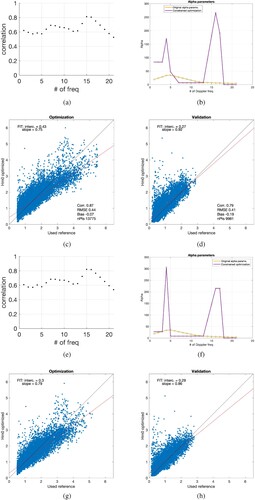
The set of 21 α parameters obtained through the least squares-constrained fitting (Figure 6b) for period D2, roughly reflects the behaviour of the correlation (Figure 6a); it is worth mentioning that the shape of the constrained α set (represented by a red line in Figure 6b) is quite different if compared to the one of the unconstrained α set (the one applied by default by the WERA software, indicated by an orange line).

Applying these α coefficients to the second-order spectral energies of period D2, a new Hm0_HFR time series is obtained. The new time series, Hm0_HFRopt1, is characterised by an increased correlation coefficient with Hm0_CMS; in particular, strongly reduced Root Mean Squared Error (RMSE) and bias are noticeable with respect to the original dataset (Table 2). Thus, the Hm0_CMS vs Hm0_HFRcal scatterplot cloud appears quite well aligned to the 1:1 line (Figure 6c and Table 2). By applying the obtained α coefficients to the spectral energies of period D1 (i.e. the validation period) resulting Hm0_HFRcal present a slightly reduced correlation coefficient, but a reduced RMSE and bias (Table 2) with a resulting good alignment along the 1:1 line (Figure 6d and Table 2).

Table 2. Correlation coefficients, RMSE, bias and coefficients (slope and intercept) of linear regression before optimisation and after it for both periods D1 and D2, with Hm0_CMS and Hm0_buoy as references.

Period	Sub-range	#points		corr		RMSE		bias
		Model	Buoy	Model	Buoy	Model	Buoy	Model	Buoy
D2	before optimisation	13775	13844	0.86	0.87	0.85	0.76	0.67	0.62
	after constr. optim.			0.87	0.88	0.44	0.37	−0.07	−0.02
D1	before validation	9981	9982	0.80	0.83	0.50	0.47	0.40	0.35
	after constr. valid.			0.79	0.82	0.41	0.36	−0.19	−0.16

5.3. Results with HFR data calibrated with in-situ data from buoy

The same optimisation procedure has been applied using Hm0_buoy data as reference. The shape of the α-coefficient curve (Figure 6f) is very similar to that obtained with modelled Hm0 as reference (Figure 6b). In general, there is an improvement of correlation coefficients and RMSEs after optimisation (Table 2), except for correlation when applying the new α coefficients to period D1. This improvement results in an alignment of data along the 1:1 line (Figure 6g,h and Table 2). In addition, the results achieved are slightly better than those previously obtained. The correlations at the 21 doppler frequencies (Figure 6e) are similar to those obtained using Hm0_CMS-P3 as reference data. For both the optimisation and the validation periods also the RMSE are lower than those previously retrieved (Table 2).

6. Discussion

Calibration of the WERA wave data by an optimisation procedure using as reference the Hm0 data from both a buoy and model, leads to an improvement in the data quality, with an increase in correlation coefficients, but more importantly with a decrease in RMSE. Qualitatively, the results obtained with both Hm0 references are very similar. However, the results obtained with the Hm0_buoy as reference are slightly better than those obtained with Hm0_CMS, even though the buoy is not in the radar field and the model grid point used is closer to the P3 radar point. This is related to the extrinsic limit of the adopted model. Indeed, the wave analyses and forecasts for the Mediterranean Sea are produced by the HCMR Production Unit by means of the WAM wave model which is a regional model that covers the entire Mediterranean basin. This kind of model is developed and optimised only for open-waters. For example, the data assimilation scheme uses satellite altimetry data which are less reliable in coastal areas. Moreover, the grid resolution (1/24° LON-LAT) is too coarse to properly capture the coastal wave hydrodynamics; the wind field is itself modelled from the ECMWF atmospheric model which is not focused on wind modelling in the coastal area.

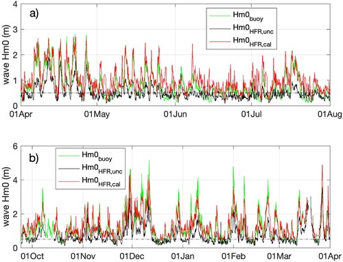
For all these reasons, we use Hm0 from the buoy as the main term for comparison with the radar data in this discussion. On the other hand, measuring wave motion with a system of 8 antennas raises a number of problems that seem to be partially solved by the optimisation procedure. Indeed, if we consider the time series of Hm0 before and after the calibration process (Figure 7), the peaks in Hm0_HFR, which were previously not detected in the uncalibrated radar measurements, are well reproduced by the optimised Hm0_HFR, even if in some cases they are still slightly underestimated. Even when the correlation computed over the entire calibrated Hm0_HFR dataset vs Hm0_buoy slightly improves to 0.88, the RMSE drops from 0.60 m before optimisation to 0.36 m after optimisation.

Figure 7. Time series of Hm0 from buoy and from radar, both uncalibrated and optimised, for period D1 (a) and D2 (b). Time series has been split into two panels and a 7-points moving average has been applied to Hm0_HFR for readability (pay attention that the vertical scale is not the same in the two panels).

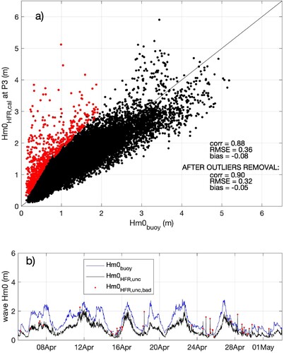
The improvement can also be seen in Figure 8(a), where it is evident that the calibrated Hm0_HFR are fairly well aligned along the 1:1 line (slope = 0.80, intercept = 0.31 m). There are some outliers corresponding to values in the Hm0_buoy below 2 m, that are overestimated by the HFR (3.3% of the total). These values correspond mainly to spikes in the original time series, but which are not flagged with instrumental quality control index (Figure 8b); this suggests that more detailed QC/QA procedures need to be further investigated.

Figure 8. (a) Scatter plot of calibrated Hm0_HFR at P3 versus Hm0_buoy for the complete period considered; the outliers are indicated in red. (b) zoom of the Hm0_buoy and Hm0_HFR,unc timeseries for the period 5/4/21–3/5/21 with the outliers in (a) marked as red points.

To understand the extent to which the new time series are able to capture the highest peaks, the correlation coefficients and RMSE is calculated for events in different ranges of Hm0. These ranges are: (i) 0.5–1.3 m, which are two functioning limits of WERA referring to the ‘noise threshold’ and the ‘limit to get wave direction’ respectively; (ii) 1.3–2 m, where the upper limit refers to the 90th percentile of the significant waves measured by the buoy and (iii) > 2 m. In general, the correlation between Hm0_buoy and Hm0_HFR,unc for Hm0 greater than 1.3 m is 0.74 with an RMSE of 1.02 m, while the correlation between Hm0_buoy and Hm0_HFR,cal remains almost the same (0.75) but the RMSE decreases significantly to 0.44 m, indicating an overall improvement in capturing the highest peaks. When Hm0 is divided into smaller classes (Table 3), it is clear that the correlation coefficient for both the 0.5–1.3 m and 1.3–2 m ranges remain almost unchanged after optimisation, which does not indicate a significant improvement, although the RMSE decreases significantly only for the second range. For Hm0 greater than 2 m, however, both correlation and RMSE are consistently improved. This fact suggests that the optimisation has produced a concrete improvement in the detection of the highest peaks. However, Figure 7 shows that for events greater than 2 m, there is still an underestimation of Hm0 in some cases.

Table 3. Correlation coefficients and RMSE between Hm0 from radar and from buoy, calculated over the entire dataset, before and after optimisation, considering different ranges for Hm0.

	Hm0HFR,unc - Hm0buoy		Hm0HFR,cal - Hm0buoy
	R	RMSE (m)	R	RMSE (m)
0.5 m ≤ Hm0 < 1.3 m	0.61	0.40	0.62	0.30
1.3 m ≤ Hm0 < 2 m	0.41	0.78	0.42	0.37
Hm0 ≥ 2 m	0.61	1.30	0.67	0.53

It is therefore important to highlight that the wave buoy is essential for the calibration of the HFR systems, even if this buoy is not designed for calibration purposes.

7. Conclusions

This study shows that an improved spectral significant wave height dataset can be obtained by calibrating data from a non-optimally configured HFR system. A reliable spectral significant wave height dataset from a radar system in addition to a point wave buoy is important because HFR measurements cover a fairly large area of the sea surface in the coastal zone and are useful for operational purposes.

This study shows that a significant gain in data quality and representativeness can be achieved if a constrained least-square adjustment is performed using a reference dataset (from a model or a wave buoy) to recalculate the coefficients used to convert measured HFR spectral energies into spectral significant wave heights. Better results are obtained with buoy data as a reference than with model data. In both cases, it appears that this first calibration phase, although still a preliminary step, has produced encouraging results that highlight the great potential of HFR systems for coastal areas, even if longer periods are required for calibration and comparison purposes. In addition, a direct comparison of the measured power/wave energy spectra from the wave buoy and the HFR should be performed in the near future, as this could further improve the calculation of a set of tailored coefficients and allow a more accurate assessment of the spectral significant wave heights of the radar system.

The quality of HFR data could be improved even if the buoy is not designed for calibration purposes. The use of a dedicated calibration wave buoy for a short period of time (no more than two years) could be very useful to obtain even better radar wave height measurements. In this framework, a calibration buoy should be designed to make direct spectral measurements needed to determine the calibration parameters for the HFR. Finally, future plans include the installation of a second HFR system to provide 2D maps of both wave height and wave direction.

Acknowledgements

We thank Roberto Gomez from Helzel Messtechnik GmbH for the help in the implementation of the applied method and for fruitful discussions regarding obtained results. We also thank Catalina Reyes Suarez for her help in downloading the data in the very first phase of the work, and Giovanni Giacalone, Ignazio Fontana and Pietro Calandrino for the technical support in the HFR maintenance. We thank the anonymous reviewers which allowed us to improve the manuscript. This study has been conducted using E.U. Copernicus Marine Service Information; dxoi: https://dxoi.org/10.25423/cmcc/medsea_analysisforecast_wav_006_017_medwam3. Author contributions. All the authors contributed to data provision; LU, FC, SA, GC, VC, AO, CLR developed the concept for the paper; LU performed the calibration calculation; FC and LU wrote the initial version of the text, and all authors commented on and revised the text and approved the final.

Disclosure statement

No potential conflict of interest was reported by the author(s).

Additional information

Funding

This study was partially funded by the European Union INTERREG VA Italia-Malta project, i-WaveNET (project code C2-3.2-106).

Notes on contributors

L. Ursella

L. Ursella Graduated in Physics at the University of Trieste (1994). She has been a researcher at OGS since 1995, working on circulation, especially basin-scale processes (seasonal and annual variability), mesoscale phenomena, and tidal processes, including those related to atmospheric events and river discharge. In addition, she is dedicated to the study of thermohaline properties and the computation of water and nutrient transports and fluxes, also related to zooplankton, their movements and the carbon cycle. Her work focuses on validation, analysis and interpretation of Eulerian and Lagrangian data. She has several experiences in oceanographic campaigns in national and international projects using CTDs, fixed and moving ship ADCP, current meters, drifters, floats. Study areas: Adriatic Sea, Eastern Mediterranean Sea, Arctic, Antarctic and Gulf of Mexico.

S. Aronica

S. Aronica is permanent Researcher in technologies and sensors for the marine and maritime environment at National Research Council of Italy. Graduated in Electronic Engineering at the Palermo University. He attended a high formation master in Protection of the Marine Environment and Oceanography. PhD in Energetic achieved in 2008 at the Palermo University, Italy. He is head of the multidisciplinary research group TESMA, dedicated to the study of Marine Technologies and Sensors, at the CNR Institute for the Study of Anthropic Impacts and Sustainability in the Marine Environment. He is also Coordinator of different research projects as principal investigator or working package leader. Main Research interests for marine ecology, marine environment monitoring, oceanography, Environmental modelling.

V. Cardin

V. Cardin is a physical oceanographer and senior researcher, currently serving as head of the Physical Oceanography Group in the Oceanography Section. She is particularly interested in air-sea interactions and the analysis of physical and biochemical data to characterise long-term changes in the Adriatic and Mediterranean Sea in response to climate change. She is currently co-chair of the Mediterranean Oceanographic Network of Ocean Observing Systems (MonGOOS). Since 2006, she has been the principal investigator of the EMSO-ERIC Regional Facility in the Southern Adriatic. As an OGS representative, she participates in several national and European tables such as EMSO (European Multidisciplinary Sea Floor and water column Observatory), ICOS (Integrated Carbon Observing System) and EuroGOOS (European Global Ocean Observing System). He has extensive experience participating in various national and European projects. With more than 400 days at sea, he has participated in several oceanographic campaigns in the Mediterranean, Pacific and Antarctic, most of them as a chief scientist. He is the author of more than 50 articles published in peer-reviewed journals, as wellas numerous communications and conference proceedings.

G. Ciraolo

G. Ciraolo is a Full professor at the University of Palermo. He read Hydraulics and Hydrology in Italy both as a graduate and a PhD. The main expertise regards monitoring the environment with a special attention to the sea-water quality in coastal areas and sea state monitoring using HF radars and models. He is a lecturer on application of remote-sensing techniques to hydrology and water quality and coastal engineering.

D. Deponte

D. Deponte, Electronic Engineering degree from the University of Trieste. Collaborates with OGS since 1995, with a permanent position in the oceanography department since 2001. Was involved in many national/international project (scientific/services) for activity related to physical oceanography monitoring/measurements also as responsible/coordinator. He has participated in many scientific expeditions aboard research vessels also in polar areas. Was involved in the design, implementation, management of monitoring systems in deep waters (mooring) and coastal systems with real time data transmission (coastal buoys) ranging from hardware, software and data processing.

C. Lo Re

C. Lo Re is a coastal engineer specialising in hydraulics and marine and coastal engineering. He holds a Master of Science degree in Civil Engineering from the University of Palermo and was a PhD student between 2006 and 2008. The subject of the doctoral thesis was coastal engineering and in particular the numerical modelling of the swash zone and run-up. He received the Ph.D. degree from the University of Palermo after the final thesis of the original thesis "Shoreline oscillation in the swash zone" and has been conducting research in the field of coastal erosion phenomena and shoreline identification for many years. He is currently a Technologist-Researcher at ISPRA (Italian Institute for Environmental Protection and Research) and works in a group that manages the Italian Wave Buoy Network. He has recently been involved in two INTERREG projects with ISPRA and participates in several working groups within ISPRA, including the National Climate Change Adaptation Plan and the Environmental Data Yearbook.

A. Orasi

A. Orasi, Degree on Statistics at the University "La Sapienza" of Rome-Italy PhD in "Statistic Methodology for Scientific Research" at University of Bologna-Italy. Presently, she is senior researcher at the Marine Weather Physical Parameters Monitoring and Marine Climatology Unit of ISPRA (Institute for Environmental Protection and Research) and she is involved in research and activities concerning marine coastal monitoring. Main activities are related to the:- pre-processing and post-processing analysis of wave models throughout statistical tools;- verification of marine models throughout in situ data and remote sensing observations;- elaboration of statistical analysis of meteomarine data- integrated monitoring of sea state through in situ, numerical models and remote sensing data- coordination and scientific activities in national and international projects about the physical sea state.

F. Capodici

F. Capodici is a researcher at the University of Palermo (Italy). His research field is Remote Sensing applied on both Land and Water environments (Hydrology, Precision Farming, water quality, sea surface currents and sea state monitoring). He is skilled on processing data acquired by passive and active sensors and collected through different platforms (satellites, airbornes, drones, HF coastal radars). Recently He developed models for processing sea current data collected by a network of HF coastal radars with specific emphasis on: i) data validation; ii) data gap filling, iii) lagrangian particle tracking. He is expert on HF coastal radars and since 2020 He is leading the EUROGOOS HF radar task team on data gap filling.

References

- Aouf, L., Hauser, D., Chapron, B., Toffoli, A., Tourain, C., Peureux, C., 2021. New directional wave satellite observations: towards improved wave forecasts and climate description in Southern Ocean. Geophys Res Lett 48. doi:10.1029/2020GL091187
- Ardhuin F, Stopa JE, Chapron B, Collard F, Husson R, Jensen RE, Johannessen J, Mouche A, Passaro M, Quartly GD, et al. 2019. Observing sea states. Front Mar Sci. https://doi.org/10.3389/fmars.2019.00124
- Barrick DE, Lipa BJ, Crissman RD. 1985. Mapping surface currents with CODAR. Sea Technol. 26:43–48.
- Basilone G, Bonanno A, Patti B, Mazzola S, Barra M, Cuttitta A, McBride R. 2013. Spawning site selection by European anchovy (Engraulis encrasicolus) in relation to oceanographic conditions in the Strait of Sicily. Fish Oceanogr. 22:309–323. doi:10.1111/fog.12024
- Bonanno A, Placenti F, Basilone G, Mifsud R, Genovese S, Patti B, di Bitetto M, Aronica S, Barra M, Giacalone G, et al. 2014. Variability of water mass properties in the Strait of Sicily in summer period of 1998–2013. Ocean Science. 10:759–770. doi:10.5194/os-10-759-2014
- Bonanno A, Zgozi S, Cuttitta A, el Turki A, di Nieri A, Ghmati H, Basilone G, Aronica S, Hamza M, Barra M, et al. 2013. Influence of environmental variability on anchovy early life stages (Engraulis encrasicolus) in two different areas of the central Mediterranean Sea. Hydrobiologia. 701:273–287. doi:10.1007/s10750-012-1285-8
- Campos RM, Islam H, Ferreira TRS, Guedes Soares C. 2021. Impact of heavy biofouling on a nearshore heave-pitch-roll wave buoy performance. Appl Ocean Res. 107:102500. doi:10.1016/j.apor.2020.102500
- Copernicus. 2022. Ocean state report, issue 6. Journal of Operational Oceanography. 15:1–220.
- Dean, R.G., Dalrymple, R.A., 1991. Water wave mechanics for engineers and scientists. Advanced Series on Ocean Engineering (Vol. 2). Singapore: World Scientific; p. 368. doi:10.1142/1232.
- Ferla, M., Nardone, G., Orasi, A., Picone, M., Falco, P., Zambianchi, E., 2022. Sea monitoring networks. pp. 211–235. doi:10.1007/978-3-030-82024-4_9
- Gomez R. 2019. Calibration of Hs with a reference. WERA Server Data Manager project. Heizel Internal document.
- Gomez, R., Helzel, T., Wyatt, L., Lopez, G., Conley, D., Thomas, N., Smet, S., Sicot, G., 2015. Estimation of wave parameters from HF radar using different methodologies and compared with wave buoy measurements at the Wave Hub, in: OCEANS 2015 - Genova. IEEE, pp. 1–9. doi:10.1109/OCEANS-Genova.2015.7271477
- Gurgel K-W, Essen H-H, Schlick T. 2006. An empirical method to derive ocean waves from second-order bragg scattering: prospects and limitations. IEEE J Oceanic Eng. 31:804–811. doi:10.1109/JOE.2006.886225
- Gurkel KW, Antonischski G, Essen HH, Schlick T. 1999. A new ground wave radar for remote sensing. Coast. Eng. 37:219–234. doi:10.1016/S0378-3839(99)00027-7
- Izquierdo P, Guedes Soares C, Nieto Borge JC, Rodríguez GR. 2004. A comparison of sea-state parameters from nautical radar images and buoy data. Ocean Eng. 31:2209–2225. doi:10.1016/j.oceaneng.2004.04.004
- Jensen RE, Swail V, Bouchard RH. 2021. Quantifying wave measurement differences in historical and present wave buoy systems. Ocean Dyn. 71:731–755. doi:10.1007/s10236-021-01461-0
- Lermusiaux PFJ, Robinson AR. 2001. Features of dominant mesoscale variability, circulation patterns and dynamics in the strait of sicily. Deep Sea Res Part I. 48:1953–1997. doi:10.1016/S0967-0637(00)00114-X
- le Traon PY, Álvarez Fanjul E, Behrens E, Stanev E, Staneva J. 2017. The copernicus marine environmental monitoring service: main scientific achievements and future prospects : special issue Mercator Océan Journal.
- le Traon PY, Reppucci A, Fanjul EA, Aouf L, Behrens A, Belmonte M, Bentamy A, Bertino L, Brando VE, Kreiner MB, et al. 2019. From observation to information and users: The copernicus marine service perspective. Front Mar Sci. https://doi.org/10.3389/fmars.2019.00234
- Lin, M., Yang, C., 2020. Ocean observation technologies: a review. Chin J Mech Eng (English Edition). https://doi.org/10.1186/s10033-020-00449-z
- Lorente P, Aguiar E, Bendoni M, Berta M, Brandini C, Cáceres-Euse A, Capodici F, Cianelli D, Ciraolo G, Corgnati L, et al. 2022. Coastal high-frequency radars in the Mediterranean – part 1: status of operations and a framework for future development. Ocean Science. 18:761–795. doi:10.5194/os-18-761-2022
- Lorente P, Lin-Ye J, García-León M, Reyes E, Fernandes M, Sotillo MG, Espino M, Ruiz MI, Gracia V, Perez S, et al. 2021. On the performance of high frequency radar in the western Mediterranean during the record-breaking storm gloria. Front Mar Sci. 8. doi:10.3389/fmars.2021.645762
- Novi L, Raffa F, Serafino F. 2020. Comparison of measured surface currents from high frequency (HF) and X-band radar in a marine protected coastal area of the Ligurian Sea. Toward an Integrated Monitoring System. Remote Sens (Basel). 12:3074. https://doi.org/10.3390/rs12183074
- Orasi A, Picone M, Drago A, Capodici F, Gauci A, Nardone G, Inghilesi R, Azzopardi J, Galea A, Ciraolo G, et al. 2018. HF radar for wind waves measurements in the Malta-Sicily Channel. Measurement (Lond). 128:446–454. doi:10.1016/j.measurement.2018.06.060
- Pollard J, Spencer T, Brooks S. 2019. The interactive relationship between coastal erosion and flood risk. Progress in Physical Geography: Earth and Environment. 43:574–585. doi:10.1177/0309133318794498
- Reyes E, Aguiar E, Bendoni M, Berta M, Brandini C, Cáceres-Euse A, Capodici F, Cardin V, Cianelli D, Ciraolo G, et al. 2022. Coastal high-frequency radars in the Mediterranean – part 2: applications in support of science priorities and societal needs. Ocean Science. 18:797–837. doi:10.5194/os-18-797-2022
- Reyes Suarez C, Gačić P, Drago C. 2019. Sea surface circulation structures in the Malta-Sicily Channel from remote sensing data. Water (Basel). 11:1589.
- Robinson AR, Sellschopp J, Warn-Varnas A, Leslie WG, Lozano CJ, Haley PJ, Anderson LA, Lermusiaux PFJ. 1999. The atlantic ionian stream.Journal of Marine Systems. 20:129–156.
- Rossi GB, Cannata A, Iengo A, Migliaccio M, Nardone G, Piscopo V, Zambianchi E. 2021. Measurement of sea waves. Sensors. 22:78. doi:10.3390/s22010078
- Sammari C, Millot C, Taupier-Letage I, Stefani A, Brahim M. 1999. Hydrological characteristics in the Tunisia - Sardinia - Sicily area during spring 1995. Deep-Sea ResearchI. 1671–1703. doi:10.1016/S0967-0637(99)00026-6
- Saviano S, de Leo F, Besio G, Zambianchi E, Uttieri M. 2020. Hf radar measurements of surface waves in the gulf of Naples (southeastern Tyrrhenian Sea): comparison With hindcast results at different scales. Front Mar Sci. 7. doi:10.3389/fmars.2020.00492
- Saviano S, Kalampokis A, Zambianchi E, Uttieri M. 2019. A year-long assessment of wave measurements retrieved from an HF radar network in the Gulf of Naples (Tyrrhenian Sea. western Mediterranean Sea). Journal of Operational Oceanography. 12:1–15. doi:10.1080/1755876X.2019.1565853
- Sorgente R, Olita A, Oddo P, Fazioli L, Ribotti A. 2011. Numerical simulation and decomposition of kinetic energy in the central Mediterranean: insight on mesoscale circulation and energy conversion. Ocean Science. 7:503–519. doi:10.5194/os-7-503-2011
- Sun D, Wang Y, Bai Y, Zhang Y. 2020. Ocean waves inversion based on airborne radar images with small incident angle. In: In: International Conference on Numerical Electromagnetic and Multiphysics Modeling and Optimization (NEMO). Hangzhou: IEEE MTT-S; p. 1–4.
- Tian Z, Tian Y, Wen B, Wang S, Zhao J, Huang W, Gill EW. 2020. Wave-height mapping from second-order harmonic peaks of wide-beam HF radar backscatter spectra. IEEE Trans Geosci Remote Sens. 58:925–937. doi:10.1109/TGRS.2019.2941823
- Tintoré J, Pinardi N, Álvarez-Fanjul E, Aguiar E, Álvarez-Berastegui D, Bajo M, Balbin R, Bozzano R, Nardelli BB, Cardin V, et al. 2019. Challenges for sustained observing and forecasting systems in the Mediterranean Sea. Front Mar Sci. 6. doi:10.3389/fmars.2019.00568
- Wyatt LR. 2002. An evaluation of wave parameters measured using a single HF radar system. Can J Remote Sens. 28:205–218. doi:10.5589/m02-018
- Wyatt LR, Green JJ, Middleditch A. 2011. HF radar data quality requirements for wave measurement. Coastal Eng. 58:327–336. doi:10.1016/j.coastaleng.2010.11.005