Hybrid robust disturbance rejection position-force control to adjust the motion of mobile manipulator in automatic aluminum foundry recycling industries

ABSTRACT

This study presents the development of an event-driven hybrid control for position and force tracking applied on a mobile robotic manipulator for metal recycling tasks. The suggested controller operates in a sequenced strategy starting from a fixed spot, moving the mobile device towards a targeted zone (${\Omega }_i^r$) from where the i-th piece-to-be-recycled is attainable (considering the arm manipulation). Once the event of entering the zone is completed, the mobile robot is fixed at a position, and the end-effector of the robotic arm is enforced towards the piece-to-be-recycled. When the end-effector touches the piece in a given spot (${\Omega }_i^e$), the hybrid control changes to the force tracking intending to carry the piece towards the spot (${\Omega }_i^p$) where it ill be processed. Each piece location is identified based on a vision-based system that applies deep learning tools using convolutional neural networks. A multi-physics numerical simulation illustrated the application of the developed controller in a realistic scenario, showing all the elements of the event-driven operation. To validate the suggested controller, the comparison with a robust control that works on a wide range of carrying mass confirms the operational improvement of the event-driven hybrid position and force design.

KEYWORDS:

• Disturbance rejection control
• hybrid position-force control
• mobile robotic manipulator
• adaptive controller
• recycling industry

1. Introduction

The interest in the recycling industry is growing continuously, considering the current problem of waste production that has increased with modern industrial development (Ezeah, Fazakerley, and Roberts 2013). This is particularly relevant given that almost all industries produce residual items from all their processes (Schlesinger 2006). Specifically, with the increase in public awareness of environmental topics, metal recycling has become of paramount relevance because incineration and landfilling represent a significant source of air and groundwater pollution (Grimaud, Perry, and Laratte 2016; Shinzato and Hypolito 2005). There is reported evidence that recycling has a significant fossil fuel energy efficiency. This has turned the issue of metal recycling into a problem for both the industry and the government due to the hygiene and health problems it may represent for the industrial workers and the general population (Capuzzi and Timelli 2018). In this recycling process, metal identification is a persistent challenge: an incorrect scrap inspection could increase time and cost in the process. In addition, the manual handling of metal pieces is time-wasting and may imply a relevant investment of economic and human resources. For the reasons mentioned above, automated metal recycling processes have gradually replaced the traditional method of manually sorting and processing metals, which offers increased efficiency, improved workers’ safety, and reduced environmental impact (Capuzzi and Timelli 2018).

The use of advanced technology and machinery to speed the gathering, sorting, and processing of various metals such as steel, aluminium, copper, and brass is called automated metal recycling. These automated systems are built to handle enormous amounts of scrap metal, guaranteeing that valuable resources are recovered and repurposed while reducing waste and energy usage (Schmitz 2006). The process begins by collecting scrap metal from diverse sources, such as manufacturing companies, building sites, and consumer garbage. Sensors, magnets, and conveyor belts are used in automated systems to classify gathered materials depending on their magnetic characteristics and content. This sorting step allows for the separation of ferrous metals from non-ferrous metals and other non-ferrous metals (Lu et al. 2022). Today, many technological methods have been generated for automatic metal sorting; some of these options are:

• Eddy Current Separation: This technique relies on the principle of electromagnetic induction. An eddy current separator creates an alternating magnetic field, which induces electrical currents in conductive materials. When non-ferrous metals pass through, they experience repulsive forces that cause them to be ejected from the stream. Eddy current separators are particularly effective in separating aluminium, copper, brass, and other non-ferrous metals from mixed materials.

• Optical Sorting: Optical sorting systems use advanced sensors, cameras, and image processing algorithms to identify and separate non-ferrous metals based on their optical properties. These systems can detect differences in colour, shape, and reflectivity of materials, enabling accurate identification and sorting of various metals. Optical sorting separates different non-ferrous metal types, including aluminium, copper, zinc, and alloys.

• X-ray Transmission Sorting: X-ray transmission sorting systems utilise X-ray technology to determine materials’ atomic density and composition. These systems can differentiate between metals and non-metallic materials by analysing the X-ray attenuation characteristics. This method is especially effective in separating heavy non-ferrous metals from lighter materials, such as lead and tungsten.

• Induction Sorting: Induction sorting technology uses electromagnetic fields to induce electrical currents in conductive materials. By analysing the induced currents and their response to the applied field, induction sorters can distinguish between various metals. This method is commonly used for sorting copper, brass, aluminium, and other non-ferrous metals.

• Near-Infrared (NIR) Sorting: Near-infrared sorting systems utilise sensors that emit and detect near-infrared light to analyse the molecular structure of materials. Different non-ferrous metals exhibit distinct near-infrared absorption patterns, allowing for their identification and separation. NIR sorting is particularly effective in sorting aluminium, copper, and stainless steel materials.

Notice that all the previous sorting options are often combined or integrated into comprehensive automatic handling systems like robotic manipulators to achieve optimal results in precise classification and sorting. Speed and adaptability, enhancing the efficiency and effectiveness of the sorting operation, are the main design criteria of such systems. The main applications of robots are to pick and place identified objects and then grasp-specific metals based on their shape, size, or other characteristics, enabling accurate sorting and organisation into designated containers or conveyor belts. When vision systems are included in the feedback loop of the mobile manipulator, variations in colour, texture, patterns, or other visual features can be determined to establish the composition and quality of metals, aiding in more accurate sorting, among others. Unfortunately, there are some limits to robotic systems employed in metal recycling, such as their efficient conjunction with automatic control rules to accomplish the work because most of such systems only give force or position controls when sorting metals. This signifies flaws in the robot’s operation when removing metal from its place and placing it on the recycling conveyor belt. These deficiencies are derived from the changes the robot undergoes in its composition when carrying a metal that does not always have the same physical properties, mechanical design, or automatic motion. As a result, there are limitations in their application, i.e. they can be applied only in particular tasks, increased operating costs due to an increase in the energy required to operate, and operating risks due to unwanted movements that can lead to risks to human safety.

As one may identify, there is a significant necessity for developing controlled robotic systems that could be robust enough to operate under two working scenarios: the first one centred on solving the position tracking in the task space, and the second one focused on operating under the mass variation at the end-effector when the object to be recycled must be carried. Notice that the transient from the first to the second state is defined by the event when the mobile manipulator grasps the object. Hence, under the adequate mechanical configuration and the practical selection of electrical components to instrument the manipulator, there is a significant necessity for implementing an automatic controller that works in both scenarios, using the grasping event as a trigger for changing the controller’s objective (and its structure in consequence).

Reports show that the hybrid control offers stability and decreases the number of control signal updates (Branicky, Borkar, and Mitter 1994; Lennartson et al. 1996). As a result, the computational load decreases simultaneously with the energy consumption. Implementing these controllers could consider aperiodic sensing, communication, and computation crucial for controlling complex cyber-physical systems such as the recycling robotic manipulator (Koutsoukos et al. 2000). In the proposed hybrid control approaches, the right-hand side of the controlled robotic follows a variable structure form. This condition emphasises the idea of using hybrid control theories to design the individual controller within each stage, as well as the discrete variation of the controller when the grasping event occurs. For this reason, this paper proposes computer aid studies of a hybrid position-force control to adjust the robot’s motion in a non-ferrous metal recycling process (Yoshikawa and Sudou 1993).

The main contributions of this study are the following:

• A visual-based neural network for recyclable pieces recognition, location estimation, and object pose.

• A hybrid controller feedback operating on the neural network estimation for performing its self-navigation towards ${\Omega }_i^r$.

• The design of a tracking trajectory hybrid position force control that deals with external forces that affect the behaviour of the mobile manipulator.

The order of this manuscript is the following: Section 2 presents the central notation, and a few mathematical preliminaries are provided regarding the class of event-driven systems. Section 3 describes the problem related to the automation manipulation of objects to be recycled. Section 3 presents the considered mathematical model for the mobile robot, the associated robotic manipulator, and their dynamic characteristics, as well as the motion limitations. Section 4 presents the problem statement related to the tracking trajectory problem for mobile robotic manipulators under state restrictions considering the recycling tasks. Section 5 details the control design, including the construction of the adaptive gain form and the reasoning behind stabilising the error in the tracking space. Section presents a strategy to optimise the convergence zone for the tracking error, a positively invariant set. The same section presents a methodology that could use only the output information from the system to derive the close-loop control design. Section7 presents the numerical results showing the comparative evidence on the proposed control design and a couple of benchmark alternatives.Section 8 closes the study with some final remarks and future trends.

2. Notation and preliminaries on hybrid systems

The mathematical notations used in this work are as follows: The set of real scalars is defined by $\mathbb{R}$; the collection of non-negative real numbers is characterised by ${\mathbb{R}}_{+}$; the set of n-dimensional vectors is represented by ${\mathbb{R}}^n$; and the Euclidean norm for $\mathit{z}\in {\mathbb{R}}^n$ is indicated by $\parallel \mathit{z}\parallel$. The symbol $\mathrm{T}$ denotes a vector or matrix’s transpose, while its matrix inverse if its determinant is non-zero, is denoted by the symbol ${\mathrm{\Pi }}^{-1}$. A square matrix with all zeros is represented by the notation $0_n$, and the identity matrix with $\mathit{n}$ rows and columns is indicated by the notation $I_n$.

A hybrid system displays a combination of continuous and discrete dynamical behaviour that can switch between these modes depending on the occurrence of an event, often characterised by holonomic state constraints. In the case of the industrial robotic system for recycling tasks, continuous dynamics come into play when the robot is moving towards the object and when the robot is carrying the object before depositing it in the position where it will be processed. On the other hand, discrete dynamics are activated when the robot grasps and releases the object at the correct spot.

The mechanical section of the manipulator dynamics follows a Lagrangian model, constituting the continuous component. In contrast, the hybrid model’s discrete aspect comprises a set of impact equations that instantaneously alter the velocities of generalised variables. We adhere to the standard representation of a hybrid model.

Definition 1.

(Ames, Cousineau, and Powell 2012) The following tuple defines a non-autonomous hybrid control system:

(1) $\mathcal{H}=\left\{\mathrm{\Gamma },\mathit{D},\mathit{U},\mathit{G},\mathit{R},\mathit{FG}\right\}.$(1)

Here, the symbol $\mathrm{\Gamma }=\left(\mathit{V},\mathit{E}\right)$ represents an oriented graph with $\mathit{V}$ and $\mathit{E}$ representing sets of vertices and edges correspondingly. A source function $\mathit{sor}:\mathit{E}\to \mathit{V}$ and a target function $\mathit{tar}:\mathit{E}\to \mathit{V}$ that links an edge with its corresponding source and target, respectively, link these sets. The domain set $\mathit{D}={\left\{D_v\right\}}_{\mathit{v}\in \mathit{V}}$ where $D_v\subseteq {\mathbb{R}}^{n_v}\times {\mathbb{R}}^{k_v}$ represents a smooth manifold for ${\mathbb{R}}^{n_v}\times {\mathbb{R}}^{k_v}$ where ${\mathbb{R}}^{k_v}$ represents the control space. The set $\mathit{U}={\left\{U_v\right\}}_{\mathit{v}\in \mathit{V}}$ is the set of admissible controls with $U_v\subset {\mathbb{R}}^{k_v}$. The set $\mathit{G}={\left\{G_e\right\}}_{\mathit{e}\in \mathit{E}}$ represents the guards where $G_e\subseteq D_{\mathit{sor}(\mathit{e})}$. The set $\mathit{R}={\left\{R_e\right\}}_{\mathit{e}\in \mathit{E}}$ corresponds to the reset maps, considering that $R_e:G_e\to D_{\mathit{tar}(\mathit{e})}$ is a smooth map. In addition, the set $\mathit{FG}={\left\{(f_v,g_v)\right\}}_{\mathit{v}\in \mathit{E}}$ defines the dynamics of a controlled system (the mobile manipulator in this study) on $\mathit{x}\in D_v$ and $\mathit{u}\in U_v$, where $(f_v,g_v)$.

The permissible variations in velocity considered in the dynamics of the automated manipulator warrant the use of hybrid flows or hybrid executions as viable solutions for the hybrid system. The following definition outlines the dynamics of the hybrid system, which can be employed to describe the motion of the robotic device.

Definition 2.

Unilateral Constraints. According to the hybrid model describing the mobile manipulator, some domains and guards are derived from unilateral constraints. The definition of a unilateral constraint is given by a tuple $\mathbf{h}=(\mathit{Q},\mathit{L},\mathit{\delta })$, in which $\mathit{Q}$ denotes the configuration space (usually ${\mathbb{R}}^n$ when generalised variables are unconstrained), $\mathit{L}:\mathit{TQ}\to \mathbb{R}$ is the hyper-regular Lagrangian, and $\mathit{\delta }:\mathit{Q}\to \mathbb{R}$ represents a unilateral restriction on the configuration space, guaranteeing that the zero-level set ${\delta }^{-1}(0)$ forms a smooth subspace.

Notice that the unilateral constraint $\mathbf{h}$ determines the corresponding guard, reset map, and vector field for the continuous dynamics. Concerning the domain of the unilateral constraint, the provided guard satisfies:

(2) $\begin{array}{c}{D}_h=\left\{\left(\mathit{q},\frac{\mathit{dq}}{\mathit{dt}}\right)\in \mathit{TQ}:\mathit{h}\left(\mathit{q}\right)\ge 0\right\},\\ G_h=\left\{\left(\mathit{q},\frac{\mathit{dq}}{\mathit{dt}}\right)\in \mathit{TQ}:\mathit{h}\left(\mathit{q}\right)=0,\frac{\mathit{dh}}{\mathit{dt}}\setminus \mathit{lt}0\right\}.\end{array}$(2)

The vector $\mathit{q}\in {\mathbb{R}}^n$, represented as $\mathit{q}={\left[\begin{array}{c}{q}_i\end{array}\right]}_{\mathit{i}=1,\dots ,\mathit{n}}^{\mathrm{T}}$, describes the joint configuration of the robotic manipulator. When a unilateral constraint is only valid within specific domains of the model, particularly depending on a specific combination of generalised variables, it is referred to as a holonomic constraint, denoted as $\mathit{\eta }(\mathit{q})$ (notably excluding $\mathit{dq}/\mathit{dt}$). Holonomic constraints can be incorporated into the control system dynamics by applying LaGrange multipliers. The common procedure involves differentiating the constraint $\mathit{\eta }(\mathit{q})$, which results in the equation $\mathit{A}\left(\mathit{q}\right)\frac{\mathit{dq}}{\mathit{dt}}=0$, where $\mathit{A}\left(\mathit{q}\right)=\frac{\mathrm{\partial \eta }}{\mathrm{\partial q}}$. Consequently, the Euler-LaGrange model for the continuous dynamics of the mobile manipulator is represented as (Crampin 1981; Ortega et al. 1994):

(3) $\begin{array}{c}\mathit{M}\left(\mathit{q}\right)\frac{d^2\mathit{q}\left(\mathit{t}\right)}{\mathit{d}{t}^2}+\mathit{G}\left(\mathit{q}\left(\mathit{t}\right),\frac{\mathit{dq}\left(\mathit{t}\right)}{\mathit{dt}},\mathit{t}\right)+A^{\mathrm{T}}\left(\mathit{q}\left(\mathit{t}\right)\right){\lambda }_{\eta }\\ \left(\mathit{q}\left(\mathit{t}\right),\frac{\mathit{dq}\left(\mathit{t}\right)}{\mathit{dt}},\mathit{u}\left(\mathit{t}\right),\mathit{t}\right)=\mathit{u}\left(\mathit{t}\right),\end{array}$(3)

Here the inertia matrix is $\mathit{M}:{\mathbb{R}}^n\to {\mathbb{R}}^{\mathit{n}\times \mathit{n}}$, and the function containing the right-hand sides of the two differential equations is represented by $\mathit{G}:{\mathbb{R}}^n\times {\mathbb{R}}^n\times {\mathbb{R}}^{+}\to {\mathbb{R}}^n$. The starting conditions of (3) are represented by $\mathit{q}(0)$ and $\left(\frac{\mathit{dq}\left(0\right)}{\mathit{dt}}\right)$ respectively.

The set of direct current (DC) motors that are regulated by the control that is in line with the motor’s voltage is represented by the signal $\mathit{u}\in {\mathbb{R}}^n$. ${\lambda }_{\eta }:\mathit{TQ}\times {\mathbb{R}}^k\to {\mathbb{R}}^c$ represents the LaGrange multiplier, and ${\mathbb{R}}^c$ denotes specific model domains where constraints are in effect. By differentiating $\mathit{\eta }(\mathit{q})$ twice, the precise expression of ${\lambda }_{\eta }$ is obtained:

(4) $\frac{\mathit{dA}\left(\mathit{q}\right)}{\mathit{dt}}\frac{\mathit{dq}\left(\mathit{t}\right)}{\mathit{dt}}+\mathit{A}\left(\mathit{q}\right)\frac{d^2\mathit{q}}{\mathit{d}{t}^2}=0.$(4)

The substitution of (3) in (4) and a suitable algebraic manipulation leads to

(5) $\begin{array}{c}{\lambda }_{\eta }\left(\mathit{q},\frac{\mathit{dq}}{\mathit{dt}},\mathit{u},\mathit{t}\right)={\mathrm{\Gamma }}_A\left[\frac{\mathit{dA}\left(\mathit{q}\right)}{\mathit{dt}}\frac{\mathit{dq}}{\mathit{dt}}+\mathit{A}\left(\mathit{q}\right)M^{-1}\left(\mathit{q}\right)\mathit{u}\left(\mathit{t}\right)\right]\\ -{\mathrm{\Gamma }}_A\mathit{A}\left(\mathit{q}\right)M^{-1}\left(\mathit{q}\right)\mathit{G}\left(\mathit{q}\left(\mathit{t}\right),\frac{\mathit{dq}\left(\mathit{t}\right)}{\mathit{dt}},\mathit{t}\right),\end{array}$(5)

where ${\mathrm{\Gamma }}_A={\left[\mathit{A}(\mathit{q}){\mathit{M}}^{-1}\left(\mathit{q}\right)A^{\mathrm{T}}(\mathit{q})\right]}^{-1}$. In order to fulfil the holonomic constraint while transporting the recyclable item, the LaGrange multiplier applies force to the mobile manipulator. Both the domain and the guard sets can be defined (using the LaGrange theorem) according to the multiplier’s value as follows:

(6) $\begin{array}{c}{D}_{\eta }=\left\{\left(\mathit{q},\frac{\mathit{dq}}{\mathit{dt}}\right)\in \mathit{TQ}\times {\mathbb{R}}^k:{\lambda }_{\eta }\ge 0\right\},\\ G_{\eta }=\left\{\left(\mathit{q},\frac{\mathit{dq}}{\mathit{dt}}\right)\in \mathit{TQ}:{\lambda }_{\eta }=0,\frac{\mathit{d\eta }\left(\mathit{q}\right)}{\mathit{dt}}\setminus \mathit{lt}0\right\}.\end{array}$(6)

The controlled system is defined by applying the additional force, represented by the LaGrange multiplier. This is represented by:

(7) $\begin{array}{c}\frac{d}{\mathit{dt}}{\xi }_1\left(\mathit{t}\right)={\xi }_2\left(\mathit{t}\right),\\ \frac{d}{\mathit{dt}}{\xi }_2\left(\mathit{t}\right)=\mathit{f}\left({\xi }_1\left(\mathit{t}\right),{\xi }_2\left(\mathit{t}\right)\right)+\mathit{g}\left({\xi }_1\left(\mathit{t}\right)\right)\mathit{u}\left(\mathit{t}\right)+\mathit{\eta }\left({\xi }_1\left(\mathit{t}\right),{\xi }_2\left(\mathit{t}\right),\mathit{t}\right),\end{array}$(7)

where ${\xi }_1=\mathit{q}$ and ${\xi }_2=\mathit{dq}/\mathit{dt}$ define the states of the mobile manipulator with ${\xi }_1(0)$ and ${\xi }_2(0)$ defined in (3). The functions $\mathit{f}:{\mathbb{R}}^n\times {\mathbb{R}}^n\to {\mathbb{R}}^n$ and $\mathit{g}:{\mathbb{R}}^n\to {\mathbb{R}}^{\mathit{n}\times \mathit{n}}$ are:

(8) $\begin{array}{c}\mathit{f}=-M^{-1}\left({\xi }_1\right)\left[\mathit{G}\left({\xi }_1,{\xi }_2,\mathit{t}\right)-A^{\mathrm{T}}\left({\xi }_1\right){\mathrm{\Gamma }}_A\frac{dA\left({\xi }_1\right)}{\mathit{dt}}{\xi }_2\right]\\ +M^{-1}\left({\xi }_1\right)A^{\mathrm{\top }}\left({\xi }_1\right){\mathrm{\Gamma }}_A\mathit{A}\left({\xi }_1\right)M^{-1}\left({\xi }_1\right)\mathit{G}\left({\xi }_1,{\xi }_2,\mathit{t}\right),\\ \mathit{g}=M^{-1}\left({\xi }_1\right)\left(I_{\mathit{n}\times \mathit{n}}-{\mathrm{\Gamma }}_A\mathit{A}\left({\xi }_1\right)M^{-1}\left({\xi }_1\right)\right].\end{array}$(8)

The nonlinear vector field $\mathit{f}$ satisfies the Lipschitz condition locally, with the fixed positive constant $L_f$ (Poznyak 2008).

The term $\mathit{\eta }:{\mathbb{R}}^n\times {\mathbb{R}}^n\times {\mathbb{R}}^{+}\to {\mathbb{R}}^n$ represents the effects of external perturbations and internal uncertainties. The model includes this term to consider a more realistic version of the mobile manipulator.

Assumption 1.

The admissible class of uncertainties – perturbations $\mathit{\eta }$ belongs to the following admissible set

(9) $\begin{array}{c}\mathit{f}=-M^{-1}\left({\xi }_1\right)\left[\mathit{G}\left({\xi }_1,{\xi }_2,\mathit{t}\right)-A^{\mathrm{T}}\left({\xi }_1\right){\mathrm{\Gamma }}_A\frac{dA\left({\xi }_1\right)}{\mathit{dt}}{\xi }_2\right]\\ +M^{-1}\left({\xi }_1\right)A^{\mathrm{\top }}\left({\xi }_1\right){\mathrm{\Gamma }}_A\mathit{A}\left({\xi }_1\right)M^{-1}\left({\xi }_1\right)\mathit{G}\left({\xi }_1,{\xi }_2,\mathit{t}\right),\\ \mathit{g}=M^{-1}\left({\xi }_1\right)\left(I_{\mathit{n}\times \mathit{n}}-{\mathrm{\Gamma }}_A\mathit{A}\left({\xi }_1\right)M^{-1}\left({\xi }_1\right)\right].\end{array}$(9)

The symbol $\mathrm{\Theta }$ is a compact, convex set such that $0\in \mathrm{\Theta }$. To characterise the movement of the mobile manipulator near around the constraint set that contains $\mathit{\eta }$, it is not sufficient to include the LaGrange multiplier. The so-called kinematic constraint, which specifies the link between velocities before and after carrying the object to be recycled, explains this behaviour.

Definition 3.

A tuple $\mathit{\kappa }=\left\{Q_s,Q_t,\mathit{M},\mathit{\vartheta },\mathit{\iota },\mathit{J}\right\}$ defines the configuration spaces of the source domain and target domain, which are denoted by the following terms $Q_s$ and $Q_t$, respectively. Complementary, $\mathit{M}:Q_s\cup J^{-1}\left(Q_t\right)\to {\mathbb{R}}^{\mathit{s}\times \mathit{s}}$ is the manipulator inertia matrix where $\mathit{s}=\mathit{dim}\left(Q_s\cup J^{-1}\left(Q_t\right)\right)$, $\mathit{\vartheta }:Q_s\cup J^{-1}\left(Q_t\right)$ is a smooth enough vector field which typically defines the position of the final element of an open kinematic chain, $\mathit{\iota }:Q_s\cup J^{-1}\left(Q_t\right)$ is and embedding with push-forward ${\iota }^{\ast }:\mathit{T}{Q}_s\to \mathit{T}\left(Q_s\cup J^{-1}\left(Q_t\right)\right)$ and $\mathit{J}$ is an invertible matrix to relabel generalised coordinates in the domain attained after the constraint manifold is left.

The vector-valued function $\mathit{s}$ should consider the entire set of $\mathit{d}$ constraints of both the unilateral and holonomic natures if they exist. The so-called canonical projection needs to be taken into account in the case of manipulator movement. This canonical projection complies with the equation $\mathit{\pi }:Q_s\cup J^{-1}\left(Q_t\right)\to J^{-1}\left(Q_t\right)$, which necessitates the use of the composite map $\mathit{\pi }\ast :\mathit{T}{Q}_s\cup J^{-1}\left(Q_t\right)$. The impact equations can be introduced using kinematic constraints.

Definition 4.

The rigid impacts of the mobile robot’s end-effector with the handled object yield a set of possible discrete jumps over the unilateral and/or holonomic constraints. Formally, these effects can be represented as impulses at the precise locations that the constraints define. In the embedded space $Q_s\cup J^{-1}\left(Q_t\right)$, let us consider the kinematic constraint $\mathit{\kappa }=\left\{Q_s,Q_t,\mathit{M},\mathit{\vartheta },\mathit{\iota },\mathit{J}\right\}$ and the generalised coordinates $\mathit{q}$. Next, let us define a map $\mathit{P}:\mathit{T}{Q}_s\cup J^{-1}\left(Q_t\right)\to \mathit{T}\left(Q_t\right)\left(J^{-1}\right)$, which describes the velocities following impact, and is described by

(10) $\begin{array}{c}\mathit{P}\left(\mathit{q}\left(\mathit{t}\right),\frac{\mathit{dq}\left(\mathit{t}\right)}{\mathit{dt}}\right)=\frac{\mathit{dq}\left(\mathit{t}\right)}{\mathit{dt}}-\\ M^{-1}\left(\mathit{q}\left(\mathit{t}\right)\right)E^{\mathrm{\top }}\left(\mathit{q}\left(\mathit{t}\right)\right){\left(\mathit{E}\left(\mathit{q}\left(\mathit{t}\right)\right){\mathit{M}}^{-1}\left(\mathit{q}\left(\mathit{t}\right)\right)E^{\mathrm{\top }}\left(\mathit{q}\left(\mathit{t}\right)\right)\right)}^{-1}\mathit{E}\left(\mathit{q}\left(\mathit{t}\right)\right)\frac{\mathit{dq}\left(\mathit{t}\right)}{\mathit{dt}},\end{array}$(10)

where $\mathit{E}\left(\mathit{q}\right)=\frac{\mathrm{\partial \kappa }}{\mathrm{\partial q}}$. The map that resets the coordinates in the target domain is defined by $\mathit{R}:\mathit{T}{Q}_s\to \mathit{T}{Q}_t$ and satisfies

(11) $\begin{array}{c}\mathit{R}\left(q_s\left(\mathit{t}\right),\frac{d{q}_s\left(\mathit{t}\right)}{\mathit{dt}}\right)=\left[\begin{array}{cc}\mathit{J}& 0\\ 0& \mathit{J}\end{array}\right]{\pi }^{\ast }\left[\begin{array}{c}\mathit{\iota }\left(q_s\right)\\ \mathit{P}\left({\iota }^{\ast }\left(q_s\left(\mathit{t}\right),\frac{d{q}_s\left(\mathit{t}\right)}{\mathit{dt}}\right)\right)\end{array}\right].\end{array}$(11)

The regular movement of the mobile manipulator during the individual object handling cycle enforces two independent stages (because no dynamic transition is considered when the object is grasped). The active device belongs to a class of hybrid systems with holonomic constraints defined by the transition between stages. The mobile manipulator’s mechanical section was acquired to explain the robotic device’s continuous flow within each step, both before and following the grasping. This simplified model could complete the controller design suggested in this study.

3. The mobile manipulator and the changing scenario for aluminium recycling

The mobile manipulator considered in this study comprises a wheeled mobile (skid steering configuration with four independent wheels) robot with a differential configuration and a 7-degree-of-freedom robotic manipulator. This device operates in a non-structured scenario where the objects to be recycled (tyre rims in the example considered in this study) can be placed anywhere in the working procedure. Figure 1 shows a sample of the working procedure, including a feasible organisation of the objects and the mobile robotic device.

Figure 1. Motion example of the mobile manipulator showing the tasks that must be completed before grasping the object, during the contact, and after carrying it.

Render of the operative scenario for the mobile manipulator in different times of task development.

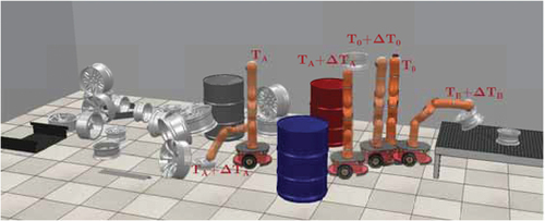
Figure 1 demonstrates an overlapped sequence of the mobile manipulator performing diverse activities in the working cycle from an initial position at them $T_0$ to a final position at time $T_0+\mathrm{\Delta }{T}_0$. Within this time window, the manipulator must move the end-effector to locate the following object that must be collected. Once the object has been located, the mobile manipulator must move towards the detected object to be recycled in a period defined by $T_A$ after $T_0+\mathrm{\Delta }{T}_0$. In this period, the manipulator must attain a specific region near the object from where it is attainable by the manipulator. Once the manipulator enters the mentioned region, then the manipulator must move to catch the object within a given period defined by $T_A+\mathrm{\Delta }{T}_A$. Notice that the robotic dynamics’ right-hand side changes now, considering the object’s handling. Once this process has ended with grasping the next object to be recycled, the robot must move towards a region form where the mobile manipulator can release the handled object to be further processed. Such part of the process must be completed after a time $T_B$ after the mobile manipulator reaches the region from which the recycled object can be released. After a time $T_B+\mathrm{\Delta }{T}_B$, the object must be located at the correct stop from where it will be processed. This task ends an entire cycle for a given specific object.

According to the motion dynamics shown in Figure 1, there are two sequential stages. The first one comprehended between $T_0$ and $T_A+\mathrm{\Delta }{T}_A$, and the second one started at $T_A+\mathrm{\Delta }{T}_A$ and ended at $T_B+\mathrm{\Delta }{T}_B$. The working cycle is completed for each set of two sequential stages.

4. Model of the mobile manipulator

This section describes the mathematical model of the mobile manipulator, which is a coupled system comprising the mobile autonomous terrestrial vehicle (ATV) and the robotic manipulator. The motion details, the state restrictions, and the potential modification in each of the stages of the working cycle are explained.

4.1. Autonomous terrestrial vehicle

To describe the position of the ATV in the working environment depicted in Figure 1, two motion reference frames were defined:

1. Inertial Coordinate System: This coordinate system is a global frame fixed in the ATV’s working environment. The position for this frame is defined by the coordinates tuple $(x_0,y_0,z_0)$.

2. Robot Coordinate System (relative): This frame is attached to the ATV centre of mass, and it is denoted by the coordinates tuple $(x_{\mathit{rm}},y_{\mathit{rm}},z_{\mathit{rm}})$.

Figure 2 displays the configuration of both reference frameworks and the matching set of variables that specify the mobile manipulator’s motion. An additional weight is placed over the ATV to balance the centre of gravity on the mid-point on the axis between wheels, coinciding with the first rotating axis for the first joint in the arm.

Figure 2. Scheme of the robot with all its frames.

Render of the mobile manipulator with all its joints reference frameworks.

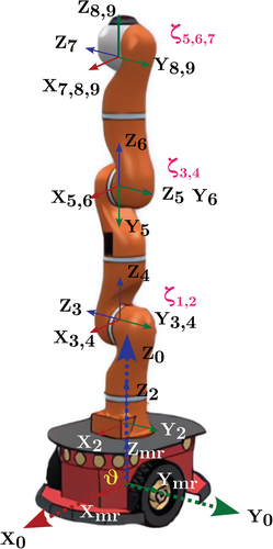
We assume that the robot’s centre of mass, designated as point $\mathit{C}$, is positioned along the axis of symmetry. As illustrated in Figure 2, the robot’s position and orientation in the Inertial Frame can be represented as $q_0={\left[\begin{array}{ccc}{x}_0& y_0& \mathit{\theta }\end{array}\right]}^{\mathrm{T}}$.

Given that $z_0=z_{\mathit{rm}}$ in our design, we assumed no temporal fluctuation over $\mathit{z}$. Hence, the triplet $q_{\mathit{rm}}={\left[\begin{array}{ccc}{\mathit{x}}_{\mathit{rm}}& y_{\mathit{rm}}& {\theta }_{\mathit{rm}}\end{array}\right]}^{\mathrm{T}}$ represents the position of any material point on the robot in the robot frame; $q_I={\left[\begin{array}{ccc}{x}_I& y_I& {\theta }_I\end{array}\right]}^{\mathrm{T}}$ represent the position of any material point on the robot with respect to the inertial reference frame. The coordinates of the specified point in the inertial frame and robot frame, respectively, make up the components of this vector.

The following transformation relates to these coordinates:

(12) $q_I=\mathit{R}(\mathit{\theta })q_{\mathit{rm}},$(12)

Here $\mathit{R}(\mathit{\theta })$ is the orthogonal rotation matrix with respect to the $\mathit{z}$-axis (Spong and Vidyasagar 1989).

This transformation defines the motion relationship between frames.

(13) $\frac{d}{\mathit{dt}}{q}_I(\mathit{t})=\mathit{R}(\mathit{\theta }(\mathit{t}))\frac{d}{\mathit{dt}}{q}_{\mathit{rm}}(\mathit{t}).$(13)

4.1.1. Kinematic model

Here, we demonstrate that the motion of the selected ATV can be described by two non-holonomic constraint equations, which are derived by making two key assumptions:

1. No lateral slip motion restriction that implies the ATV can only travel in a curved motion (forward and backward) with a minimum curvature radius but not sideways. This condition in the relative frame indicates that the velocity of the centre-point A along the lateral axis is zero at any moment during the motion task, that is $y_{\mathit{rm}}=\frac{d}{\mathit{dt}}{y}_{\mathit{rm}}=0$, $\mathrm{\forall t}\ge 0$. These two conditions can be represented by the following single non-holonomic condition:

   (14) $-\frac{d}{\mathit{dt}}{x}_0\text{cdotsin}\left(\mathit{\theta }\right)+\frac{d}{\mathit{dt}}{y}_0\text{cdotcos}\left(\mathit{\theta }\right)=0.$(14)

2. The pure rolling restriction denotes the fact that each wheel has just one point of contact with the ground ($\mathit{p}$). The wheel does not slip along its longitudinal axis ($x_r$) and does not skid along its orthogonal axis ($y_r$).

The velocities of the contact points in the relative frame $v_R$ and $v_L$ are connected to the velocities $\frac{d}{\mathit{dt}}{\varphi }_R$ and $\frac{d}{\mathit{dt}}{\varphi }_L$ of the right (R) and left (L) wheels by:

(15) $v_R=\mathit{\rho }\frac{d}{\mathit{dt}}{\varphi }_R{v}_L=\mathit{\rho }\frac{d}{\mathit{dt}}{\varphi }_L,$(15)

here $\mathit{\rho }$ is the radius of each wheel. These velocities can be estimated in the inertial frame as a function of the velocities of the ATV centre-point A:

(16) $\begin{array}{c}\frac{d}{\mathit{dt}}{x}_{\mathit{p},\mathit{R}}=\frac{d}{\mathit{dt}}{x}_0+\mathit{Lcos}\left(\mathit{\theta }\right)\frac{d}{\mathit{dt}}\mathit{\theta },\\ \frac{d}{\mathit{dt}}{y}_{\mathit{p},\mathit{R}}=\frac{d}{\mathit{dt}}{y}_0-\mathit{Lsin}\left(\mathit{\theta }\right)\frac{d}{\mathit{dt}}\mathit{\theta },\\ \frac{d}{\mathit{dt}}{x}_{\mathit{p},\mathit{L}}=\frac{d}{\mathit{dt}}{x}_0-\mathit{Lcos}\left(\mathit{\theta }\right)\frac{d}{\mathit{dt}}\mathit{\theta },\\ \frac{d}{\mathit{dt}}{y}_{\mathit{p},\mathit{L}}=\frac{d}{\mathit{dt}}{y}_0+\mathit{Lsin}\left(\mathit{\theta }\right)\frac{d}{\mathit{dt}}\mathit{\theta }.\end{array}$(16)

The linear velocity of the ATV in the robot frame, which is the average of the linear velocities of the two wheels, is the linear velocity of each driving wheel in the robot frame.

(17) $\mathit{v}=\frac{v_R+v_L}{2}=\frac{\rho }{2}\frac{d}{\mathit{dt}}\left({\phi }_R+{\phi }_L\right),$(17)

and the angular velocity of the ATV is

(18) $\mathit{\omega }=\frac{v_R-v_L}{2\mathit{L}}=\frac{\rho }{2\mathit{L}}\frac{d}{\mathit{dt}}\left({\phi }_R-{\phi }_L\right).$(18)

Considering the case that the material port $q_{\mathit{rm}}$ corresponds to point A (implying that $\mathit{v}=\frac{d}{\mathit{dt}}{q}_{\mathit{rm}}$), the linear and angular velocities of the ATV can be expressed as follows:

(19) $\frac{d}{\mathit{dt}}\left[\begin{array}{c}{x}_{\mathit{rm}}\\ y_{\mathit{rm}}\\ {\theta }_{\mathit{rm}}\end{array}\right]=\frac{1}{2\mathit{L}}\left[\begin{array}{cc}\mathit{L\rho }& \mathit{L\rho }\\ 0& 0\\ \mathit{\rho }& -\mathit{\rho }\end{array}\right]\frac{d}{\mathit{dt}}\mathit{\phi },\mathit{\phi }=\left[\begin{array}{c}{\phi }_R\\ {\phi }_L\end{array}\right].$(19)

The translational and angular velocities can also be obtained in the inertial frame as follows:

(20) $\frac{d}{\mathit{dt}}{q}_I=\frac{d}{\mathit{dt}}\left[\begin{array}{c}{x}_I\\ y_I\\ {\theta }_I\end{array}\right]=\frac{1}{2\mathit{L}}\left[\begin{array}{cc}\mathit{L\rho }cos\mathit{\theta }& \mathit{L\rho }cos\mathit{\theta }\\ \mathit{L\rho }sin\mathit{\theta }& \mathit{L\rho }sin\mathit{\theta }\\ \mathit{\rho }& -\mathit{\rho }\end{array}\right]\frac{d}{\mathit{dt}}\mathit{\phi }.$(20)

The forward kinematic model of the TAR is represented by Equation (20)(20) $\frac{d}{\mathit{dt}}{q}_I=\frac{d}{\mathit{dt}}\left[\begin{array}{c}{x}_I\\ y_I\\ {\theta }_I\end{array}\right]=\frac{1}{2\mathit{L}}\left[\begin{array}{cc}\mathit{L\rho }cos\mathit{\theta }& \mathit{L\rho }cos\mathit{\theta }\\ \mathit{L\rho }sin\mathit{\theta }& \mathit{L\rho }sin\mathit{\theta }\\ \mathit{\rho }& -\mathit{\rho }\end{array}\right]\frac{d}{\mathit{dt}}\mathit{\phi }.$(20) .

Given the contact points’ velocities and the corresponding constraint equations can be rewritten as follows with $\mathit{q}={\left[x_0,y_0,\mathit{\theta },{\phi }_R,{\phi }_L\right]}^{\mathrm{T}}$:

(21) $\mathrm{\Lambda }\left(\mathit{q}\right)\frac{d}{\mathit{dt}}\mathit{q}=0,\mathrm{\Lambda }\left(\mathit{q}\right)=\left[\begin{array}{ccccc}-\mathit{sin}\left(\mathit{\theta }\right)& \mathit{cos}\left(\mathit{\theta }\right)& 0& 0& 0\\ \mathit{cos}\left(\mathit{\theta }\right)& \mathit{sin}\left(\mathit{\theta }\right)& \mathit{L}& -\mathit{\rho }& 0\\ \mathit{cos}\left(\mathit{\theta }\right)& \mathit{sin}\left(\mathit{\theta }\right)& -\mathit{L}& 0& -\mathit{\rho }\end{array}\right].$(21)

4.1.2. Dynamic modeling of the ATV system

For the ATV that is moving in a two-dimensional plane, the potential energy is constant, and hence, the dynamic model of such a vehicle can be presented as follows:

(22) $\frac{d}{\mathit{dt}}\frac{\mathrm{\partial T}\left(\mathit{t}\right)}{\mathrm{\partial }\dot{q}}-\frac{\mathrm{\partial T}\left(\mathit{t}\right)}{\mathrm{\partial q}}=Q_{\mathit{no}-\mathit{pot}}\left(\mathit{t}\right)+{\mathrm{\Lambda }}^{\mathrm{T}}\left(\mathit{q}\left(\mathit{t}\right)\right)\mathit{\lambda }.$(22)

The dynamic model is necessary for both the creation of motion control algorithms and the simulation analysis of the ATV motion. The following equations of motion can describe the dynamics in the presence of non-holonomic restrictions:

(23) $\begin{array}{c}{M}_{\mathit{ATV}}\left(\mathit{q}\left(\mathit{t}\right)\right)\frac{d^2\mathit{q}\left(\mathit{t}\right)}{\mathit{d}{t}^2}+C_{\mathit{ATV}}\left(\mathit{q}\left(\mathit{t}\right),\frac{\mathit{dq}\left(\mathit{t}\right)}{\mathit{dt}}\right)\frac{d}{\mathit{dt}}\mathit{q}\left(\mathit{t}\right)=\\ B_{\mathit{ATV}}\left(\mathit{q}\left(\mathit{t}\right)\right)u_{\mathit{ATV}}\left(\mathit{t}\right)-{\mathrm{\Lambda }}^{\mathrm{\top }}\left(\mathit{q}\left(\mathit{t}\right)\right)\mathit{\lambda }\left(\mathit{t}\right)+\mathit{\vartheta }\left(\frac{d}{\mathit{dt}}\mathit{q}\left(\mathit{t}\right),\mathit{q}\left(\mathit{t}\right),\mathit{t}\right),\end{array}$(23)

where $M_{\mathit{ATV}}:{\mathbb{R}}^5\to {\mathbb{R}}^{5\times 5}$ is the inertia matrix, $C_{\mathit{ATV}}:{\mathbb{R}}^5\to {\mathbb{R}}^{5\times 5}$ is the centripetal and Coriolis matrix, $B_{\mathit{ATV}}:{\mathbb{R}}^5\to {\mathbb{R}}^2$ is the input matrix, and $u_{\mathit{ATV}}$ is the input vector. The term $\mathit{\vartheta }:{\mathbb{R}}^5\times {\mathbb{R}}^5\times {\mathbb{R}}^{+}$ represents all the uncertainties and the perturbations affecting the ATV motion. Furthermore, the expressions for the matrices $M_{\mathit{ATV}}$, $C_{\mathit{ATV}}$, and $B_{\mathit{ATV}}$: are the following:

(24) $\begin{array}{c}{M}_{\mathit{ATV}}\left(\mathit{q}\right)=\left[\begin{array}{ccccc}\mathit{m}& 0& -\mathit{md}{s}_{\theta }& 0& 0\\ 0& \mathit{m}& -\mathit{md}{c}_{\theta }& 0& 0\\ -\mathit{md}{s}_{\theta }& -\mathit{md}{c}_{\theta }& \mathit{I}& 0& 0\\ 0& 0& 0& I_{\omega }& 0\\ 0& 0& 0& 0& I_{\omega }\end{array}\right],\\ C_{\mathit{ATV}}\left(\mathit{q},\dot{q}\right)=\left[\begin{array}{ccccc}0& 0& -\mathit{md}\frac{d}{\mathit{dt}}\mathit{\theta }{c}_{\theta }& 0& 0\\ 0& 0& -\mathit{md}\frac{d}{\mathit{dt}}\mathit{\theta }{s}_{\theta }& 0& 0\\ 0& 0& 0& 0& 0\\ 0& 0& 0& 0& 0\\ 0& 0& 0& 0& 0\end{array}\right],{\text{breakB}}_{ATV}^{\mathrm{\top }}\left(\mathit{q}\right)=\left[\begin{array}{ccccc}1& 0& 0& 0& 0\\ 0& 1& 0& 0& 0\end{array}\right],\end{array}$(24)

where $\mathit{m}=m_c+2m_w$ is the total mass of the ATV and is equal to the mass of the MR without the driving wheels and actuators ($m_c$) plus the mass of each driving wheel with the actuator ($m_w$), $\mathit{I}=I_c+m_c{d}^2+2m_w{L}^2+2I_m$ is the total equivalent inertia; here $I_{\mathrm{c}}$ is the moment of inertia of the MR about the vertical axis through the centre of mass, $I_w$ is the moment of inertia of each driving wheel with a motor about the wheel axis, and $I_m$ is the moment of inertia of each driving wheel with a motor about the wheel diameter. Introducing the relationship between $\mathit{q}$ and $\mathit{\phi }$, the dynamics of $\mathit{q}$ and $\mathit{\phi }$ are related by

(25) $\frac{d}{\mathit{dt}}\mathit{q}=\mathit{S}\left(\mathit{q}\right)\frac{d}{\mathit{dt}}\mathit{\phi },S^{\mathrm{\top }}\left(\mathit{q}\right)=0.5\left[\begin{array}{ccccc}\mathit{\rho }{c}_{\theta }& \mathit{\rho }{s}_{\theta }& \frac{\rho }{L}& 2& 0\\ \mathit{\rho }{c}_{\theta }& \mathit{\rho }{s}_{\theta }& -\frac{\rho }{L}& 0& 2\end{array}\right].$(25)

Given that $\mathit{S}$ is in the null space of the restriction matrix ${\mathrm{\Lambda }}^{\mathrm{T}}$, then

(26) $\frac{d^2}{\mathit{d}{t}^2}\mathit{q}=\frac{d}{\mathit{dt}}\mathit{S}\left(\mathit{q}\right)\frac{d}{\mathit{dt}}\mathit{\phi }+\mathit{S}\left(\mathit{q}\right)\frac{d^2}{\mathit{d}{t}^2}\mathit{\phi }.$(26)

The substitution of (26) in (23) leads to

(27) $\begin{array}{c}{M}_{\mathit{ATV}}\left(\mathit{q}\left(\mathit{t}\right)\right)\left(\frac{d}{\mathit{dt}}\mathit{S}\left(\mathit{q}\left(\mathit{t}\right)\right)\frac{d}{\mathit{dt}}\mathit{\phi }\left(\mathit{t}\right)+\mathit{S}\left(\mathit{q}\left(\mathit{t}\right)\right)\frac{d^2}{\mathit{d}{t}^2}\mathit{\phi }\left(\mathit{t}\right)\right)+C_{\mathit{ATV}}\text{break}\left(\mathit{q}\left(\mathit{t}\right),\frac{\mathit{dq}\left(\mathit{t}\right)}{\mathit{dt}}\right)\frac{d}{\mathit{dt}}\mathit{q}\left(\mathit{t}\right)=\\ B_{\mathit{ATV}}\left(\mathit{q}\left(\mathit{t}\right)\right)u_{\mathit{ATV}}\left(\mathit{t}\right)-{\mathrm{\Lambda }}^{\mathrm{\top }}\left(\mathit{q}\left(\mathit{t}\right)\right)\mathit{\lambda }\left(\mathit{t}\right)\text{break}+\mathit{\vartheta }\left(\frac{d}{\mathit{dt}}\mathit{q}\left(\mathit{t}\right),\mathit{q}\left(\mathit{t}\right),\mathit{t}\right).\end{array}$(27)

Multiplying both sided by $S^{\mathrm{T}}$ and using its relationship with matrix $\mathrm{\Lambda }$, one gets

(28) $\begin{array}{c}{M}_{\mathit{ATV}}\left(\mathit{q}\left(\mathit{t}\right)\right)\left(\frac{d}{\mathit{dt}}\mathit{S}\left(\mathit{q}\left(\mathit{t}\right)\right)\frac{d}{\mathit{dt}}\mathit{\phi }\left(\mathit{t}\right)+\mathit{S}\left(\mathit{q}\left(\mathit{t}\right)\right)\frac{d^2}{\mathit{d}{t}^2}\mathit{\phi }\left(\mathit{t}\right)\right)+C_{\mathit{ATV}}\text{break}\left(\mathit{q}\left(\mathit{t}\right),\frac{\mathit{dq}\left(\mathit{t}\right)}{\mathit{dt}}\right)\frac{d}{\mathit{dt}}\mathit{q}\left(\mathit{t}\right)=\\ B_{\mathit{ATV}}\left(\mathit{q}\left(\mathit{t}\right)\right)u_{\mathit{ATV}}\left(\mathit{t}\right)-{\mathrm{\Lambda }}^{\mathrm{\top }}\left(\mathit{q}\left(\mathit{t}\right)\right)\mathit{\lambda }\left(\mathit{t}\right)\text{break}+\mathit{\vartheta }\left(\frac{d}{\mathit{dt}}\mathit{q}\left(\mathit{t}\right),\mathit{q}\left(\mathit{t}\right),\mathit{t}\right).\end{array}$(28)

This form represents the model to be controlled simultaneously with the robotic arm. Notice that (28) can be represented as follows

(29) $\begin{array}{c}\frac{d}{\mathit{dt}}{\phi }_a\left(\mathit{t}\right)={\phi }_b\left(\mathit{t}\right),\\ \frac{d}{\mathit{dt}}{\phi }_b\left(\mathit{t}\right)=\mathcal{F}\left({\phi }_a\left(\mathit{t}\right),{\phi }_b\left(\mathit{t}\right)\right)+\mathcal{G}\left(q_a\left(\mathit{t}\right)\right)u_{\mathit{RM}}\left(\mathit{t}\right)+\mathrm{\Xi }\left(\mathit{q}\left(\mathit{t}\right),\frac{d}{\mathit{dt}}\mathit{q}\left(\mathit{t}\right),\mathit{t}\right).\end{array}$(29)

Here ${\phi }_a=\mathit{\varphi }$ and ${\phi }_b=\frac{d}{\mathit{dt}}\mathit{\varphi }$, while $\mathcal{F}:{\mathbb{R}}^5\times {\mathbb{R}}^5\to {\mathbb{R}}^2$ and $\mathcal{G}:{\mathbb{R}}^5\to {\mathbb{R}}^{2\times 2}$ defines the inner dynamics of the ATV system with $\mathcal{F}\left(\mathit{q},\frac{d}{\mathit{dt}}\mathit{q}\right)=-M_{\phi }^{-1}\left(\mathit{q}\right)\left(C_{\phi }\left(\mathit{q},\frac{d}{\mathit{dt}}\mathit{q}\right){\phi }_b\right)$ and $\mathcal{G}\left(\mathit{q}\right)=M_{\phi }^{-1}\left({\phi }_a\right)$. The term $\mathrm{\Xi }:{\mathbb{R}}^5\times {\mathbb{R}}^5\times {\mathbb{R}}^{+}\to {\mathbb{R}}^2$ represents the effect of uncertainties and perturbations induced by the arm and some non-modelled elements in the recycling facility. The term $\mathrm{\Xi }\left(\mathit{q},\frac{d}{\mathit{dt}},\mathit{t}\right)$ satisfies the following inclusion (implying the corresponding bounds for perturbations as well as uncertainties), according to the mechanical structure of the robotic arm:

(30) $∥\mathrm{\Xi }\left(\mathit{q},\frac{d}{\mathit{dt}}\mathit{q},\mathit{t}\right)∥\le {\mathrm{\Xi }}_0,{\mathrm{\Xi }}_0>0.$(30)

4.2. Robotic arm

The proposed robotic arm device defines six active joints (degrees of freedom). The Euler-LaGrange equations, a theory of analytical mechanics, are used to establish such a device’s mathematical structure (considering the joint motion’s mechanical dynamics). The aforementioned model’s time dependence establishes the acceleration dynamical model in the chosen generalised coordinates ${\zeta }_a$ and ${\zeta }_b$ as

(31) $\begin{array}{c}\frac{d}{\mathit{dt}}{\zeta }_a\left(\mathit{t}\right)={\zeta }_b\left(\mathit{t}\right),\\ \frac{d}{\mathit{dt}}{\zeta }_b\left(\mathit{t}\right)=\mathit{f}\left({\zeta }_a\left(\mathit{t}\right),{\zeta }_b\left(\mathit{t}\right)\right)+g_a\left({\zeta }_a\left(\mathit{t}\right)\right)u_{\mathit{RM}}\left(\mathit{t}\right)+\mathit{\xi }\left({\zeta }_a\left(\mathit{t}\right),{\zeta }_b\left(\mathit{t}\right),\mathit{t}\right),\end{array}$(31)

whereas ${\zeta }_b$ relates to the time derivative of the generalised coordinates, the variable ${\zeta }_a$ refers to the generalised coordinates that describe the motion of the manipulator articulations. In this case, $\mathit{f}:\mathcal{Z}\times \mathcal{Z}\to {\mathbb{R}}^6$, defines the drifted dynamics associated to the manipulator device; the control associated dynamics are characterised by $g_a:\mathcal{Z}\to {\mathbb{R}}^{6\times 6}$; and the dynamics associated with the control are defined by $\mathit{\xi }:\times \times \mathbb{R}\to {\mathbb{R}}^6$ represents a modelling error’s impact on the manipulator dynamics and an abstraction of external perturbations; $u_{\mathit{RM}}\in {\mathbb{R}}^6$ corresponds to the control action’s impact on the manipulator dynamics. $\mathit{\xi }\left({\zeta }_b,{\zeta }_a,\mathit{t}\right)$ satisfies the following inclusion (implying the corresponding bounds for perturbations as well as uncertainties), according to the mechanical structure of the robotic arm:

(32) $∥\mathit{\xi }\left({\zeta }_b(\mathit{t}),{\zeta }_a(\mathit{t}),\mathit{t}\right)∥\le {\xi }_0,{\xi }_0>0.$(32)

In view of (32) notice that $\mathit{\xi }\left({\zeta }_b(\mathit{t}),{\zeta }_a(\mathit{t}),\mathit{t}\right)\in {\mathcal{L}}_{\mathrm{\infty }}^n$.

Taking into account the fundamentals of the Euler-LaGrange approach, both vector functions $\mathit{f}$, and $g_a$ are described as:

(33) $\begin{array}{c}\mathit{f}\left({\zeta }_a,{\zeta }_b\right)=-M^{-1}\left({\mathrm{\Lambda }}^{\mathrm{T}}\left({\zeta }_a\right)\mathit{\lambda }+\mathit{C}\left({\zeta }_a,{\zeta }_b\right){\zeta }_b\right),\\ g_a\left({\zeta }_a\right)=M^{-1}\left({\zeta }_a\right)\mathit{B}\left({\zeta }_a\right).\end{array}$(33)

Taking into account the Euler-LaGrange basis, the condition ${∥g_b\left({\zeta }_a\right)∥}_{\mathrm{\Gamma }}\le g_b^0,g_b^0>0$ for all ${\zeta }_a$ and the corresponding positive matrix $\mathrm{\Gamma }$, using the Frobenius norm.

The mechanical robotic arm establishes motion restrictions for ${\zeta }_a$ and ${\zeta }_b$. Without loss of generality, the next class of asymmetric constraints is considered in this study. Such motion limitations are represented as:

(34) $\begin{array}{c}\mathrm{\Omega }=\left\{{\zeta }_{\mathit{a},\mathit{t}}|-\mathrm{\infty }<{\zeta }_{a,i}^{-}<{\zeta }_{\mathit{a},\mathit{i}}<{\zeta }_{a,i}^{+}<+\mathrm{\infty }\right\}.\end{array}$(34)

The feasible positions for the manipulator end-effector could be calculated using direct kinematics and the corresponding Jacobian in light of the motion coordinate restrictions taken into account in (34). It should be noted that the control issue can be resolved by considering the end-effector’s motion, which may be connected to the joint dynamics when the inverse kinematics of the AM is used.

4.3. Integrated dynamics of the mobile robot

Based on the individual models of the ATV and the robotic arm, we can present the aggregated model represented as follows using the following definitions ${\varsigma }_a^{\mathrm{T}}=\left[{\phi }_a^{\mathrm{T}},{\zeta }_a^{\mathrm{T}}\right]$ and ${\varsigma }_b^{\mathrm{T}}=\left[{\phi }_b^{\mathrm{T}},{\zeta }_b^{\mathrm{T}}\right]$:

(35) $\begin{array}{c}\mathit{f}\left({\zeta }_a,{\zeta }_b\right)=-M^{-1}\left({\mathrm{\Lambda }}^{\mathrm{T}}\left({\zeta }_a\right)\mathit{\lambda }+\mathit{C}\left({\zeta }_a,{\zeta }_b\right){\zeta }_b\right),\\ g_a\left({\zeta }_a\right)=M^{-1}\left({\zeta }_a\right)\mathit{B}\left({\zeta }_a\right).\end{array}$(35)

Here, we used the notation $u_{\mathit{\sigma }(\mathit{t})}$ to establish the application of the variable control form $\mathit{\sigma }(\mathit{t})$ when the task scenario changes from the approach to the object to its handling towards the deployment. Hence, $\mathit{\sigma }(\mathit{t})=1$ in the first scenario, while $\mathit{\sigma }(\mathit{t})=2$ when the second state happens.

4.4. On the reference trajectories for the mobile manipulator

To define the problem to be solved in this study, introduce the variable ${\mathrm{\Delta }}_a$ corresponding to the tracking error between the trajectories of the combined robot (ATV and RM) and a suitable set of references ${\varsigma }_a^{\ast }\in {\mathbb{R}}^8$. The reference dynamics satisfies the following differential equation

(36) $\begin{array}{c}\frac{d}{\mathit{dt}}{\varsigma }_a^{\ast }\left(\mathit{t}\right)={\varsigma }_b^{\ast }\left(\mathit{t}\right),\\ \frac{d}{\mathit{dt}}{\varsigma }_b^{\ast }\left(\mathit{t}\right)={\mathrm{\Psi }}_{\mathit{\sigma }\left(\mathit{t}\right)}\left({\varsigma }_a^{\ast }\left(\mathit{t}\right),{\varsigma }_b^{\ast }\left(\mathit{t}\right),\mathit{t}\right).\end{array}$(36)

with ${\varsigma }_a^{\ast }\in {\mathbb{R}}^8$ and its derivative ${\varsigma }_b^{\ast }\in {\mathbb{R}}^8$. The initial conditions are given vectors in (36). The function ${\mathrm{\Psi }}_{\mathit{\sigma }(\mathit{t})}:{\mathbb{R}}^8\times {\mathbb{R}}^8\times {\mathbb{R}}^{+}\to {\mathbb{R}}^8$ is a Lipschitz function that defines the reference acceleration within each stage of the robotic motion for the ATV and the RM. Notice that this function is proposed to change depending on the mobile manipulator’s active mode, given that the referred trajectories may not be differentiable in the edges, even if they are continuous.

Various methods can address the challenge of designing reference trajectories within each continuous domain. This issue is commonly referred to as trajectory planning for robotic systems. Among the widely used approaches is the Bezier polynomial, which involves defining a set of controls to determine a Bezier curve with points from $P_0$ to $P_{\nu }$, where $\mathit{\nu }$ denotes its order (e.g. $\mathit{\nu }=1$ for linear, $\mathit{\nu }=2$ for quadratic, etc.). The first and last control points always correspond to the curve’s endpoints, representing the initial conditions after resetting and the achieved final state in each domain. However, the intermediate control points, if present, typically do not lie on the curve. This paper explores an alternative approach to generating reference trajectories. The concept involves constructing the reference trajectory by interpolating sigmoid functions, following the methodology proposed in (Cruz, Luviano-Juárez, and Chairez 2014). These functions are differentiable multiple times, allowing for the regulation of their transient trajectory from one steady state to another. Each component of the reference trajectories can be estimated using the following sigmoidal representation. The specific form of the sigmoid function employed in this article is:

(37) $\begin{array}{c}{\varsigma }_a^{\ast }\left(\mathit{t}\right)=|{\varsigma }_{a,i}^{\ast }\left(\mathit{t}\right){|}_{\mathit{i}=1,...,\mathit{\nu }},\\ {\varsigma }_{a,i}^{\ast }\left(\mathit{t}\right)=\frac{a_i}{1+b_i{e}^{\left(\mathit{t}-{\mathit{t}}_{\mathit{k}.\mathit{i}}\right)}}+c_i,\mathrm{\forall t}\in \left[T_i,T_i+T_{\mathit{i},\mathit{w}}\right],\end{array}$(37)

where the scalar parameters $a_i$, $b_i$, and $c_i$ are present, and $t_{\mathit{k},\mathit{i}}$ denotes the sigmoid function’s inflection point. The reader is directed to the study given in (Cruz, Luviano-Juárez, and Chairez 2014) for more information on the design method for the reference trajectories using sigmoid functions.

By using a derivation procedure, $h_i(\mathit{t})=a_i{b}_i{e}^t(b_i{e}^t-1)\times {\left(1+b_i{e}^t\right)}^{-3}$, one can easily obtain the expression of each component for the reference function $\mathit{\delta }$ based on the structure of the sigmoid function proposed in (37). In the vector field $\mathit{\delta }$, the $\mathit{i}-\mathit{th}$ component is the function ${\delta }_i\left(\mathit{t}\right)$.

5. Problem formulation

Based on the integrated dynamics presented in (35) and the reference trajectories (36), the dynamics of the tracking error ${\mathrm{\Delta }}_a$ is governed by the following differential equations:

(38) $\begin{array}{c}\frac{d}{\mathit{dt}}{\mathrm{\Delta }}_a\left(\mathit{t}\right)={\mathrm{\Delta }}_b\left(\mathit{t}\right),\\ \frac{d}{\mathit{dt}}{\mathrm{\Delta }}_b\left(\mathit{t}\right)={\mathrm{\Psi }}_{\mathit{\sigma }\left(\mathit{t}\right)}\left({\varsigma }_a^{\ast }\left(\mathit{t}\right),{\varsigma }_b^{\ast }\left(\mathit{t}\right),\mathit{t}\right)-\left(\mathit{F}\left({\varsigma }_a\left(\mathit{t}\right),{\varsigma }_b\left(\mathit{t}\right)\right)\text{break}+\mathit{G}\left({\varsigma }_a\left(\mathit{t}\right)\right)u_{\mathit{\sigma }\left(\mathit{t}\right)}\left(\mathit{t}\right)+\mathit{\eta }\left({\varsigma }_a\left(\mathit{t}\right),{\varsigma }_b\left(\mathit{t}\right),\mathit{t}\right)\right).\end{array}$(38)

hich have a practically stable equilibrium point on the origin within each time window for each continuous mode. According to the definition of the hybrid system presented in (1), Figure 3 shows the configuration of the mobile manipulator throughout the interaction with the object to be handled. The sense of the vertices is characterised by the scenarios shown here and the edges shown as the interconnection lines. The set $\mathit{U}$ is characterised by both controllers operating in each scenario and the dynamics $\mathit{FG}$, which are defined by the ordinary differential Equation (38)(38) $\begin{array}{c}\frac{d}{\mathit{dt}}{\mathrm{\Delta }}_a\left(\mathit{t}\right)={\mathrm{\Delta }}_b\left(\mathit{t}\right),\\ \frac{d}{\mathit{dt}}{\mathrm{\Delta }}_b\left(\mathit{t}\right)={\mathrm{\Psi }}_{\mathit{\sigma }\left(\mathit{t}\right)}\left({\varsigma }_a^{\ast }\left(\mathit{t}\right),{\varsigma }_b^{\ast }\left(\mathit{t}\right),\mathit{t}\right)-\left(\mathit{F}\left({\varsigma }_a\left(\mathit{t}\right),{\varsigma }_b\left(\mathit{t}\right)\right)\text{break}+\mathit{G}\left({\varsigma }_a\left(\mathit{t}\right)\right)u_{\mathit{\sigma }\left(\mathit{t}\right)}\left(\mathit{t}\right)+\mathit{\eta }\left({\varsigma }_a\left(\mathit{t}\right),{\varsigma }_b\left(\mathit{t}\right),\mathit{t}\right)\right).\end{array}$(38) . The set of guards and resets is defined by the limits illustrated as ellipsoids in the centre of the referred figure, with resets defined by null jumps, given the reference trajectories’ continuity (and the no necessary differentiability on the edges).

Figure 3. Operating diagram for the MR considering the definition of the hybrid system used in this study.

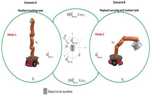
According to the mobilisation problem, the edges of the hybrid system are defined by $\mathit{E}=\left\{E_1\left({\left.\mathrm{\Delta }\right|}_{\mathit{\sigma }(\mathit{t})=1}\right),E_2\left({\left.\mathrm{\Delta }\right|}_{\mathit{\sigma }(\mathit{t})=2}\right)\right\}$. Here ${\left.\mathrm{\Delta }\right|}_{\mathit{\sigma }(\mathit{t})=1}$ and ${\left.\mathrm{\Delta }\right|}_{\mathit{\sigma }(\mathit{t})=2}$ define the tracking error for the corresponding scenario characterised with $\mathit{\sigma }(\mathit{t})=1$ or $\mathit{\sigma }(\mathit{t})=2$. The detected edges are

(39) $\setminus \mathit{matrix}{E}_1\left({\left.\mathrm{\Delta }\right|}_{\mathit{\sigma }\left(\mathit{t}\right)=1}\right)=||{\mathrm{\Delta }}_{\mathit{\sigma }\left(\mathit{t}\right)=1}||={\rho }_{\mathit{r},1},\setminus \mathit{break}{E}_2\left({\left.\mathrm{\Delta }\right|}_{\mathit{\sigma }\left(\mathit{t}\right)=2}\right)\le ||{\mathrm{\Delta }}_{\mathit{\sigma }\left(\mathit{t}\right)=2}||\le {\rho }_{\mathit{r},2}.\setminus \mathit{cr}$(39)

Here ${\rho }_{\mathit{r},1}$ defines the maximum distance from where the manipulator could reach each object to be handled, while ${\rho }_{\mathit{r},2}$ establishes the distance from where the handled object could be released at the position where it will be processed in the recycling process.

The control set $\mathit{U}$ is defined by both controllers applied for the selected scenarios $\mathit{U}=\left\{u_1\left({\left.\mathrm{\Delta }\right|}_{\mathit{\sigma }(\mathit{t})=1}\right),u_2\left({\left.\mathrm{\Delta }\right|}_{\mathit{\sigma }(\mathit{t})=2}\right)\right\}$ with

(40) $\begin{array}{c}{u}_1(\mathit{t}|\mathit{k})=G^{-1}\left({\varsigma }_a(\mathit{t})\right)\left({\mathrm{\Psi }}_1\left({\varsigma }_a^{\ast }(\mathit{t}),{\varsigma }_b^{\ast }(\mathit{t}),\mathit{t}|\mathit{k}\right)-\right.\\ \left.\left(\mathit{F}\left({\varsigma }_a(\mathit{t}),{\varsigma }_b(\mathit{t})\right)-W_1\left({\left.\mathrm{\Delta }\right|}_{\mathit{\sigma }(\mathit{t})=1}(\mathit{t}|\mathit{k})\right)\right)\right)\\ u_2\left(\mathit{t}|\mathit{k}\right)=G^{-1}\left({\varsigma }_a(\mathit{t})\right)\left({\mathrm{\Psi }}_2\left({\varsigma }_a^{\ast }(\mathit{t}),{\varsigma }_b^{\ast }(\mathit{t}),\mathit{t}|\mathit{k}\right)-\right.\\ \left.\left(\mathit{F}\left({\varsigma }_a(\mathit{t}),{\varsigma }_b(\mathit{t})\right)-W_2\left({\left.\mathrm{\Delta }\right|}_{\mathit{\sigma }(\mathit{t})=2}(\mathit{t}|\mathit{k})\right)\right)\right).\end{array}$(40)

Here $V_1\left({\left.\mathrm{\Delta }\right|}_{\mathit{\sigma }(\mathit{t})=1}(\mathit{t})\right)$ and $V_2\left({\left.\mathrm{\Delta }\right|}_{\mathit{\sigma }(\mathit{t})=2}(\mathit{t})\right)$ are given by

(41) $\begin{array}{c}{W}_1\left({\left.\mathrm{\Delta }\right|}_{\mathit{\sigma }\left(\mathit{t}\right)=1}(\mathit{t}|\mathit{k})\right)=K_{\mathit{P},1}(\mathit{t}|\mathit{k})\mathrm{\Delta }\left(\mathit{t}\right)+K_{\mathit{D},1}(\mathit{t}|\mathit{k})\frac{d}{\mathit{dt}}\mathrm{\Delta }\left(\mathit{t}\right)+K_{\mathit{I},1}(\mathit{t}|\mathit{k})\text{break}\underset{\mathit{\tau }=0}{\overset{t}{\int }}\mathrm{\Delta }\left(\mathit{\tau }\right)\mathit{d\tau }\\ W_2\left({\left.\mathrm{\Delta }\right|}_{\mathit{\sigma }\left(\mathit{t}\right)=2}(\mathit{t}|\mathit{k})\right)=K_{\mathit{P},2}(\mathit{t}|\mathit{k})\mathrm{\Delta }\left(\mathit{t}\right)+K_{\mathit{D},2}(\mathit{t}|\mathit{k})\frac{d}{\mathit{dt}}\mathrm{\Delta }\left(\mathit{t}\right)\text{break}+K_{\mathit{I},2}(\mathit{t}|\mathit{k}{)}_{\tau =0}^t\mathrm{\Delta }\left(\mathit{\tau }\right)\mathit{d\tau }+K_{\mathit{II},2}(\mathit{t}|\mathit{k})\underset{\mathit{\tau }=0}{\overset{t}{\int }}\underset{\mathit{s}=0}{\overset{\tau }{\int }}\mathrm{\Delta }\left(\mathit{s}\right)\mathit{dsd\tau }.\end{array}$(41)

The gains $K_{\mathit{P},1}\in {\mathbb{R}}^{8\times 8}$, $K_{\mathit{D},1}\in {\mathbb{R}}^{8\times 8}$, and $K_{\mathit{I},1}\in {\mathbb{R}}^{8\times 8}$ that operate in the scenario related to pure tracking trajectory without payload position and the gains $K_{\mathit{P},2}\in {\mathbb{R}}^{8\times 8}$, $K_{\mathit{D},2}\in {\mathbb{R}}^{8\times 8}$, $K_{\mathit{I},2}\in {\mathbb{R}}^{8\times 8}$, and $K_{\mathit{II},2}\in {\mathbb{R}}^{8\times 8}$ working for solving the tracking in the presence of payload are state dependent. The index $\mathit{k}\in \mathbb{N}$ refers to the $\mathit{k}-\mathit{th}$ object to be handled in the recycling procedure.

The laws used to obtain the evolution of such gains are the following:

(42) $\begin{array}{c}{W}_1\left({\left.\mathrm{\Delta }\right|}_{\mathit{\sigma }\left(\mathit{t}\right)=1}(\mathit{t}|\mathit{k})\right)=K_{\mathit{P},1}(\mathit{t}|\mathit{k})\mathrm{\Delta }\left(\mathit{t}\right)+K_{\mathit{D},1}(\mathit{t}|\mathit{k})\frac{d}{\mathit{dt}}\mathrm{\Delta }\left(\mathit{t}\right)\text{break}+K_{\mathit{I},1}(\mathit{t}|\mathit{k})\underset{\mathit{\tau }=0}{\overset{t}{\int }}\mathrm{\Delta }\left(\mathit{\tau }\right)\mathit{d\tau }\\ W_2\left({\left.\mathrm{\Delta }\right|}_{\mathit{\sigma }\left(\mathit{t}\right)=2}(\mathit{t}|\mathit{k})\right)=K_{\mathit{P},2}(\mathit{t}|\mathit{k})\mathrm{\Delta }\left(\mathit{t}\right)\text{break}+K_{\mathit{D},2}(\mathit{t}|\mathit{k})\frac{d}{\mathit{dt}}\mathrm{\Delta }\left(\mathit{t}\right)+K_{\mathit{I},2}(\mathit{t}|\mathit{k}{)}_{\tau =0}^t\mathrm{\Delta }\left(\mathit{\tau }\right)\mathit{d\tau }+K_{\mathit{II},2}(\mathit{t}|\mathit{k})\underset{\mathit{\tau }=0}{\overset{t}{\int }}\underset{\mathit{s}=0}{\overset{\tau }{\int }}\mathrm{\Delta }\left(\mathit{s}\right)\mathit{dsd\tau }.\end{array}$(42)

The initial conditions for the adjustable matrices are $K_{\mathit{P},1}(0|\mathit{k})=K_{\mathit{P},1}(t_{k-1}^{-}|\mathit{k})$, $K_{\mathit{D},1}(0|\mathit{k})=K_{\mathit{D},1}(t_{k-1}^{-}|\mathit{k})$, $K_{\mathit{I},1}(0|\mathit{k})=K_{\mathit{I},1}(t_{k-1}^{-}|\mathit{k})$, $K_{\mathit{P},2}(0|\mathit{k})=K_{\mathit{P},2}(t_{k-1}^{-}|\mathit{k})$, $K_{\mathit{D},2}(0|\mathit{k})=K_{\mathit{D},2}(t_{k-1}^{-}|\mathit{k})$, $K_{\mathit{I},2}(0|\mathit{k})=K_{\mathit{I},2}(t_{k-1}^{-}|\mathit{k})$, and $K_{\mathit{II},2}(0|\mathit{k})=K_{\mathit{II},2}(t_{k-1}^{-}|\mathit{k})$. These selections imply no jumps for the evolution of the gains.

The matrices ${\mathrm{\Lambda }}_{\mathit{P},1}\in {\mathbb{R}}^{8\times 8}$, ${\mathrm{\Lambda }}_{\mathit{D},1}\in {\mathbb{R}}^{8\times 8}$, ${\mathrm{\Lambda }}_{\mathit{I},1}\in {\mathbb{R}}^{8\times 8}$, ${\mathrm{\Lambda }}_{\mathit{P},2}\in {\mathbb{R}}^{8\times 8}$, ${\mathrm{\Lambda }}_{\mathit{D},2}\in {\mathbb{R}}^{8\times 8}$, ${\mathrm{\Lambda }}_{\mathit{I},2}\in {\mathbb{R}}^{8\times 8}$, and ${\mathrm{\Lambda }}_{\mathit{II},2}\in {\mathbb{R}}^{8\times 8}$ are positive definite, constant and symmetric. The initial conditions for (42) $K_{\mathit{P},1}(0|\mathit{k})$, $K_{\mathit{D},1}(0|\mathit{k})$, $K_{\mathit{I},1}(0|\mathit{k})$, $K_{\mathit{P},2}(0|\mathit{k})$, $K_{\mathit{D},2}(0|\mathit{k})$, $K_{\mathit{I},2}(0|\mathit{k})$, and $K_{\mathit{II},2}(0|\mathit{k})$ are giving as part of the resetting process on the scenario change. Besides, the time varying gains are ${\tilde{K}}_{\mathit{II},\mathit{\sigma }}(\mathit{t}|\mathit{k})=K_{\mathit{II},\mathit{\sigma }}(\mathit{t}|\mathit{k})-K_{II}^{\ast }(\mathit{k})$, ${\tilde{K}}_{\mathit{I},\mathit{\sigma }}(\mathit{t}|\mathit{k})=K_{\mathit{I},\mathit{\sigma }}(\mathit{t}|\mathit{k})-K_I^{\ast }(\mathit{k})$, ${\tilde{K}}_{\mathit{D},\mathit{\sigma }}(\mathit{t}|\mathit{k})=K_{\mathit{D},\mathit{\sigma }}(\mathit{t}|\mathit{k})-K_D^{\ast }(\mathit{k})$, and ${\tilde{K}}_{\mathit{P},\mathit{\sigma }}(\mathit{t}|\mathit{k})=K_{\mathit{P},\mathit{\sigma }}(\mathit{t}|\mathit{k})-K_P^{\ast }(\mathit{k})$.

The matrices $P_1(\mathit{k})\in {\mathbb{R}}^{8\times 8}$, $P_1(\mathit{k})=P_1^{\mathrm{T}}(\mathit{k})$ and $P_2(\mathit{k})\in {\mathbb{R}}^{8\times 8}$, $P_2(\mathit{k})=P_2^{\mathrm{T}}(\mathit{k})$ satisfy the following Riccati-like matrix equations:

(43) $\begin{array}{c}\mathit{P}\left(\mathit{k}\right)\left(\mathbf{A}\left(\mathit{k}\right)+{\mathbf{B}\mathbf{K}}_{\sigma }^{\ast }\left(\mathit{k}\right)\right)+{\left(\mathbf{A}\left(k\right)+{\mathbf{B}\mathbf{K}}_{\sigma }^{\ast }\left(\mathit{k}\right)\right)}^{\mathrm{T}}\mathit{P}\left(\mathit{k}\right)+\mathit{P}\left(\mathit{k}\right)\mathbf{B}{\mathrm{\Sigma }}_1^{-1}\text{break}{\mathbf{B}}^{\mathrm{T}}\mathit{P}\left(\mathit{k}\right)+Q_C=0,\\ {\mathrm{{\rm Y}}}^{\mathrm{T}}(t_{\mathit{k}-1}|\mathit{k})\left(\mathit{P}\left(\mathit{k}\right)+\mathrm{\Omega }\right)\mathrm{{\rm Y}}(t_{\mathit{k}-1}|\mathit{k})-\mathit{P}\left(\mathit{k}\right)+Q_D=0,\end{array}$(43)

Here, the matrices that define the Riccati-like matrix Equations (43)(43) $\begin{array}{c}\mathit{P}\left(\mathit{k}\right)\left(\mathbf{A}\left(\mathit{k}\right)+{\mathbf{B}\mathbf{K}}_{\sigma }^{\ast }\left(\mathit{k}\right)\right)+{\left(\mathbf{A}\left(k\right)+{\mathbf{B}\mathbf{K}}_{\sigma }^{\ast }\left(\mathit{k}\right)\right)}^{\mathrm{T}}\mathit{P}\left(\mathit{k}\right)+\mathit{P}\left(\mathit{k}\right)\mathbf{B}{\mathrm{\Sigma }}_1^{-1}\text{break}{\mathbf{B}}^{\mathrm{T}}\mathit{P}\left(\mathit{k}\right)+Q_C=0,\\ {\mathrm{{\rm Y}}}^{\mathrm{T}}(t_{\mathit{k}-1}|\mathit{k})\left(\mathit{P}\left(\mathit{k}\right)+\mathrm{\Omega }\right)\mathrm{{\rm Y}}(t_{\mathit{k}-1}|\mathit{k})-\mathit{P}\left(\mathit{k}\right)+Q_D=0,\end{array}$(43) are defined by

(44) $\begin{array}{c}\mathit{P}\left(\mathit{k}\right)\left(\mathbf{A}\left(\mathit{k}\right)+{\mathbf{B}\mathbf{K}}_{\sigma }^{\ast }\left(\mathit{k}\right)\right)+{\left(\mathbf{A}\left(k\right)+{\mathbf{B}\mathbf{K}}_{\sigma }^{\ast }\left(\mathit{k}\right)\right)}^{\mathrm{T}}\mathit{P}\left(\mathit{k}\right)+\mathit{P}\left(\mathit{k}\right)\mathbf{B}{\mathrm{\Sigma }}_1^{-1}{\mathbf{B}}^{\mathrm{T}}\mathit{P}\left(\mathit{k}\right)\text{break}+Q_C=0,\\ {\mathrm{{\rm Y}}}^{\mathrm{T}}(t_{\mathit{k}-1}|\mathit{k})\left(\mathit{P}\left(\mathit{k}\right)+\mathrm{\Omega }\right)\mathrm{{\rm Y}}(t_{\mathit{k}-1}|\mathit{k})-\mathit{P}\left(\mathit{k}\right)+Q_D=0,\end{array}$(44)

The adaptive PID controller (including its variation with extended uncertainties and perturbations compensation term) is considered in this study because it is regarded as one of the best ways to control electromechanical devices due to its capacity to approach reference trajectories and reject bounded perturbations. A desirable characteristic of any controller forcing the motion of a mobile robot, such as the robotic manipulator, is the ability to reduce the energy consumed during the operation in both scenarios. This is achieved by including the adaptive gains in (41).

6. Main result on the control design method

This section presents the main result of this study regarding the controller’s design, the differential equation’s existence for the control gains, and the reason that explains the existence of the stable trajectories for the hybrid system.

6.1. Main theorem of the study

The next Theorem summarises the main results obtained in this manuscript.

Theorem 6.1.

Consider the tracking error dynamics given in (38), regulated with the law $\mathit{u}\in U_v$ proposed in (40) adjusted with the gains given in (42). Consider the assumptions regarding the admissible sets of external perturbations and uncertainties given in (30) and (32). If there exists positive definite matrices $Q_C$ and $Q_D(\mathit{k})$ such that the matrix inequality (43) has a positive definite solution $\mathit{P}(\mathit{k})$, then the trajectories of the tracing error are stable in the Lyapunov sense with respect to the zero trajectories, that is

(45) $\underset{\mathit{\kappa }\to \mathrm{\infty }}{\overline{lim}}\sum _{\mathit{k}=1}^{\kappa }\frac{1}{{\mathrm{\Pi }}_{k-1}^2}{\mathrm{\Delta }}^{\mathrm{T}}(t_{\mathit{k}-1})Q_D(\mathit{k})\mathrm{\Delta }(t_{\mathit{k}-1})\le {\lambda }_{\mathit{max}}\left\{{\mathbf{B}}^{\mathrm{T}}\left(\mathit{I}+{\mathrm{\Omega }}^{-1}\right)\mathbf{B}\right\}{\eta }_0,$(45)

where ${\mathrm{\Pi }}_{\mathit{k}-1}=t_k-t_{\mathit{k}-1}$ and $\mathrm{\Omega }$ is a positive definite matrix of appropriate dimensions.

The controller proposed in Theorem 1 assumes that both the articulation and the angular velocity for each joint can be measured simultaneously. Notice that the expression (45) can be reduced only if the matrix $\mathit{P}(\mathit{k})$ is large in some sense.

The proof of this Theorem is presented in the Appendix of this manuscript.

6.2. Optimization of convergence region

The boundedness result proposed in Theorem 1 is a consequence of the non-matched uncertainties and the presence of external perturbations that may affect the orthosis movement. The invariant ellipsoid method can minimise the bound of the convergence region (Ordaz and Poznyak 2015a, 2015b; Polyakov 2010).

Definition 5.

(Polyakov and Poznyak 2009) The proposed ellipsoid

(46) $\mathcal{E}(P_1)=\left\{\mathit{z}\in {\mathbb{R}}^n:z^{\mathrm{T}}{P}_1\mathit{z}\le 1,P_1>0\right\},$(46)

is characterised with a centre placed at the origin and the configuration positive definite matrix $P_1$ which is said to be invariant for the trajectories of the system (38) if

1. the initial condition $\mathit{z}(0)\in \mathcal{E}(P_1)$ implies $\mathit{z}(\mathit{t})\in \mathcal{E}(P_1)$ for all $\mathit{t}\ge 0$,

2. the initial condition $\mathit{z}(0)\ne \mathcal{E}(P_1)$ implies $\mathit{z}(\mathit{t})\to \mathcal{E}(P_1)$ as $\mathit{t}\to \mathrm{\infty }$.

The potential discovery of an invariant ellipsoid characterised by the matrix $P_1$, with the maximum dimensions, facilitates the minimal deviation of all conceivable trajectories from the origin. While this understanding aligns seamlessly with the outcome elucidated in (43), it necessitates the establishment of a metric or criterion for determining the magnitude of the matrix $\mathit{P}(\mathit{k})$. In this context, the trace operator serves as the chosen criterion, wherein $\mathrm{tr}\left\{\mathit{P}(\mathit{k})\right\}\to \max$ or $\mathrm{tr}\left\{\mathit{P}{(\mathit{k})}^{-1}\right\}\to \min$.

In Theorem 1, the existence of the invariant set, where the trajectories of $\mathrm{\Delta }(t_{\mathit{k}-1})$ converge, has already been established for each evaluation period ${\mathrm{\Pi }}_{\mathit{k}-1}$.

In accordance with the definition outlined in (43), the configuration matrix $\mathit{P}(\mathit{k})$ adheres to the concept of an invariant ellipsoid when taking into account the inequality (45). To determine the solution for the minimal invariant ellipsoid, the following Lemma provides sufficient conditions for designing the gain controller.

Lemma 1.

If the tupple ($\mathit{\alpha }:={\lambda }_{\mathit{max}}\left\{{\mathbf{B}}^{\mathrm{T}}\left(\mathit{I}+{\mathrm{\Omega }}^{-1}\right)\mathbf{B}\right\}{\eta }_0$, $\mathit{P}(\mathit{k})$) is a solution of the optimisation problem $\mathrm{tr}\left\{\mathit{P}(\mathit{k})\right\}\to max$, subjected to $\mathit{P}(\mathit{k})>0$, $\mathit{\alpha }>0$ and

(47) $\left[\begin{array}{cc}\mathit{P}(\mathit{k})\left(\mathbf{A}(\mathit{k})+{\mathbf{B}\mathbf{K}}_{\sigma }^{\ast }(\mathit{k})\right)+{\left(\mathbf{A}(k)+{\mathbf{B}\mathbf{K}}_{\sigma }^{\ast }(\mathit{k})\right)}^{\mathrm{T}}\mathit{P}(\mathit{k})+Q_C& \mathit{P}(\mathit{k})\\ \mathit{P}(\mathit{k})& -\mathbf{B}{\mathrm{\Sigma }}_1^{-1}{\mathbf{B}}^{\mathrm{T}}\end{array}\right]\le 0,$(47)

Then, the corresponding controller proposed in (40) guarantees that any trajectory of the system (38) converges to a quasi-minimal ellipsoid $\mathcal{E}(\mathit{P}(\mathit{k}))$ within each scenario for the mobile robot.

The proof of this Lemma follows straightforwardly from the application of the Schur complement on (43).

6.3. Output-based adaptive PID controller

The proposed solution for addressing the output-based tracking problem consists of an output feedback controller, comprising a robust exact differentiator (RED) as suggested in (Levant 1998) for obtaining velocity estimation. Additionally, a modified version of the adaptive proportional-derivative controller (APD) is employed to track reference trajectories. The velocity estimation is accomplished using this differentiator based on the Super-Twisting algorithm (STA). Employing the STA, the PID control is then selected as part of the control strategy.

(48) $\begin{array}{c}{u}_1(\mathit{t}|\mathit{k})=G^{-1}\left({\varsigma }_a\left(\mathit{t}\right)\right)\left({\mathrm{\Psi }}_1\left({\varsigma }_a^{\ast }\left(\mathit{t}\right),{\varsigma }_b^{\ast }\left(\mathit{t}\right),\mathit{t}|\mathit{k}\right)-\left.\left(\mathit{F}\left({\varsigma }_a\left(\mathit{t}\right),{\hat{\varsigma }}_{\mathit{b}}\left(\mathit{t}\right)\right)-W_1\left({\left.\hat{\mathrm{\Delta }}\right|}_{\mathit{\sigma }\left(\mathit{t}\right)=1}(\mathit{t}|\mathit{k})\right)\right)\right),\right.\\ u_2\left(\mathit{t}|\mathit{k}\right)=G^{-1}\left({\varsigma }_a\left(\mathit{t}\right)\right)\left({\mathrm{\Psi }}_2\left({\varsigma }_a^{\ast }\left(\mathit{t}\right),{\varsigma }_b^{\ast }\left(\mathit{t}\right),\mathit{t}|\mathit{k}\right)-\left.\left(\mathit{F}\left({\varsigma }_a\left(\mathit{t}\right),{\hat{\varsigma }}_{\mathit{b}}\left(\mathit{t}\right)\right)-W_2\left({\left.\hat{\mathrm{\Delta }}\right|}_{\mathit{\sigma }\left(\mathit{t}\right)=2}(\mathit{t}|\mathit{k})\right)\right)\right),\right.\end{array}$(48)

where $\hat{\mathrm{\Delta }}$ is the estimated vector of the tracking error. The application of the super-twisting algorithm (STA) as a robust and exact differentiator (RED) is based on the following description: If ${\mathbf{w}}_1\left(\mathit{t}\right)=\mathbf{r}\left(\mathit{t}\right)$, where $\mathbf{r}(\mathit{t})\in \mathbb{R}$ is the signal to be differentiated, and ${\mathbf{w}}_2(\mathit{t})=\dot{\mathbf{r}}(\mathit{t})$ represents its derivative, the following auxiliary equation is obtained under the assumption $\left|\ddot{\mathbf{r}}(\mathit{t})\right|\le {\mathbf{r}}^{+}$.

(49) $\frac{d}{\mathit{dt}}{\mathbf{w}}_1\left(\mathit{t}\right)={\mathbf{w}}_2\left(\mathit{t}\right);\frac{d}{\mathit{dt}}{\mathbf{w}}_2\left(\mathit{t}\right)=\ddot{\mathbf{r}}\left(\mathit{t}\right).$(49)

The previous differential equation is a state representation of the signal $\mathbf{r}(\mathit{t}).$ The STA algorithm to obtain the derivative of $\mathbf{r}\left(\mathit{t}\right)$ looks like

(50) $\frac{d}{\mathit{dt}}{\overline{w}}_1\left(\mathit{t}\right)={\overline{w}}_2\left(\mathit{t}\right)-{\lambda }_1\left|{\Delta }_w(\mathit{t})\right|{,}^{1/2}\text{sign}\left({\Delta }_w(\mathit{t})\right),\frac{d}{\mathit{dt}}{\overline{w}}_2\left(\mathit{t}\right)=-{\lambda }_2\text{sign}\left({\Delta }_w(\mathit{t})\right),{\Delta }_w={\overline{w}}_1\left(\mathit{t}\right)-w_1\left(\mathit{t}\right),\mathit{d}(\mathit{t})=\frac{d}{\mathit{dt}}{\overline{w}}_1\left(\mathit{t}\right)$(50)

where ${\lambda }_1,{\lambda }_2>0$ are the STA gains. Here $\mathit{d}(\mathit{t})$ is the output of the differentiator (Levant 1998). In this equation,

(51) $\mathrm{sign}(\mathit{z}):=\left\{\begin{array}{cc}1& \mathit{if}\mathit{z}>0\\ -1,1]& \mathit{if}\mathit{z}=0\\ -1& \mathit{if}\mathit{z}<0\end{array}\right.$(51)

To implement the control method proposed in this article, the algorithm shown in Figure 4 was developed. The results of this algorithm are showing in the next section.

Figure 4. Employed algorithm flow.

7. Numerical results

In this section, the results are obtained by implementing the scenario for recycling car wheels in Coppeliasim with the proposed mobile robot. To configure the scenario, Matlab and Coppeliasim were set to work in supervised synchronous mode by the API function for Matlab. The declaration of commands and functional programming was developed in Matlab. On the other hand, the speed of the robot’s active joints was measured using virtual instrumentation in Coppeliasim.

Furthermore, those results compare setting an automatic control algorithm with extended state feedback or Proportional Integral Derivative (PID) control and with a law that considers the implementation of adaptive gains over a configuration of disturbance rejection control form. The initial gains setting for the robotic device are shown in Table 1.

Table 1. Initial gain’s condition of the robotic device.

	Joint
Gain name	ATV	q1	q2	q3	q4	q5	q6	q7
KP	2.8	0.0078	0.0078	0.0078	0.0078	24.4800	23.0400	4.3200
KD	5.6	19.4400	19.6344	19.4400	19.4400	8.1600	7.6800	1.4400
KI	0.1	0.0000	0.0000	0.0000	0.0000	0.4352	0.4096	0.0768
KP	2.8	0.0039	0.0039	0.0039	0.0039	24.4800	23.0400	4.3200
KD	5.8	12.9600	13.0896	12.9600	12.9600	8.1600	7.6800	1.4400
KI	0.00005	0.0000	0.0000	0.0000	0.0000	0.4352	0.4096	0.0768
KII	0.00001	0.0000	0.0000	0.0000	0.0000	0.0218	0.0164	0.0038

As has been mentioned, the task of taking one wheel to the recycling band is developed in four stages. The first stage corresponds to the period when the mobile robot approaches the object. The second one corresponds to the period when the object is lifted. The third refers to the case when the lifted object is moved towards the conveyor. The fourth and last stage corresponds to the period when the object is released.

The application of inverse kinematics allowed us to construct the set of reference trajectories for all the joints in the Kuka robot to reach the wheel and then leave it in the recycling band. Moreover, the difference between the wheel and the home position is computed to orientate the robot and move it close to the wheel.

Each stage of the Kuka robot is executed in an elapsed time of 120 s. Those events’ trajectories and movements are shown in Figure 5. Both controllers show asymptotic convergence for the tracking errors. This fact can be appreciated in Figure 5, demonstrating that tracking errors are monotonically decreasing, specifically in those joints that change their position between the stages and in the case of those joints that have to maintain the position, the error is $\pm$ 2^°, like in the case of q_1,3,5,7.

Figure 5. Trajectory tracking for each DoF of the Kuka robot.

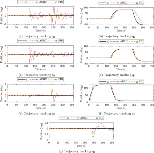
After analysing the trajectory tracking of each joint, it is possible to observe that each stage change converges to the desired position about 60 s after the start of the corresponding stage. During stage 1, developed by the manipulator, both control laws reflect a similar performance. However, during stages 2 and 3, it is possible to observe a better performance in tracking the trajectories by the proposed controller (ADRC). Although during stage 2, there is no change in the manipulator dynamics, the motion of the daughter’s joints affects the parent joints, which is why slight position changes are observed in the joints q_1,3,5,7 for $120[\mathit{sec}]\ge \mathit{t}\le 240[\mathit{sec}]$ (see Figure 6).

Figure 6. Temporal evolution of the error for each DoF of the Kuka robot.

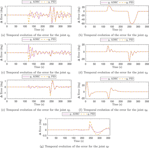
Finally, during the stage where the rin is loaded by the manipulator (third stage), it is possible to observe a more noticeable change in the proposed control law (ADRC) performance. The graphs corresponding to the error Figure 6 for $240[\mathit{sec}]\ge \mathit{t}\le 360[\mathit{sec}]$ reflect a lower error when the system has the ADRC control (magenta line). Specifically, the rin-attracting joint (q${ }_7$) exhibits lower error at the beginning and during that stage.

As part of the controllers’ performance demonstration, both the Mean Square Error (MSE) and the Error Integral (EI) per stage, controller, and joint were calculated and are presented in the Table 2 and Table 3, respectively.

Table 2. Comparison of the mean square error values for the different control laws at each stage for the Kuka robot.

	Joint MSE
Stage	q1	q2	q3	q4	q5	q6	q7	Total
ST1 - ADRC	6.855 ${\times }^{-05}$	9.203${\times }^{-06}$	8.695${\times }^{-05}$	4.703${\times }^{-05}$	1.227${\times }^{-05}$	7.802${\times }^{01}$	3.058${\times }^{-07}$	1.627${\times }^{02}$
ST1 - PID	5.391${\times }^{-05}$	1.764${\times }^{-05}$	6.820${\times }^{-05}$	5.001${\times }^{-05}$	3.444${\times }^{-05}$	7.769${\times }^{01}$	1.052${\times }^{-06}$	7.769${\times }^{01}$
ST2 - ADRC	4.048${\times }^{-02}$	9.413${\times }^{01}$	9.004${\times }^{-02}$	2.120${\times }^{01}$	1.085${\times }^{-02}$	4.726${\times }^{01}$	1.941${\times }^{-04}$	1.627${\times }^{02}$
ST2 - PID	7.661${\times }^{-02}$	9.799${\times }^{01}$	7.100${\times }^{-02}$	2.152${\times }^{01}$	4.342${\times }^{-03}$	4.615${\times }^{01}$	1.862${\times }^{-04}$	1.658${\times }^{02}$
ST3 - ADRC	1.706${\times }^{-01}$	9.677${\times }^{02}$	2.935${\times }^{-02}$	4.689${\times }^{01}$	1.165${\times }^{-01}$	1.594${\times }^{-02}$	3.086${\times }^{-02}$	1.015${\times }^{03}$
ST3 - PID	1.905${\times }^{-01}$	9.936${\times }^{02}$	1.848${\times }^{-02}$	4.950${\times }^{01}$	1.868${\times }^{-01}$	1.706${\times }^{-02}$	1.039${\times }^{-01}$	1.044${\times }^{03}$

Table 3. Comparison of the error integral values for the different control laws at each stage for the Kuka robot.

	Joint EI
Stage	q1	q2	q3	q4	q5	q6	q7	Total
ST1 - ADRC	2.056${\times }^{-03}$	2.761${\times }^{-04}$	2.609${\times }^{-03}$	1.411${\times }^{-03}$	3.680${\times }^{-04}$	2.341${\times }^{03}$	9.173${\times }^{-06}$	2.341${\times }^{03}$
ST1 - PID	1.617${\times }^{-03}$	5.292${\times }^{-04}$	2.046${\times }^{-03}$	1.500${\times }^{-03}$	1.033${\times }^{-03}$	2.331${\times }^{03}$	3.157${\times }^{-05}$	2.331${\times }^{03}$
ST2 - ADRC	1.214	2.824${\times }^{03}$	2.701	6.359${\times }^{02}$	3.256${\times }^{-01}$	1.418${\times }^{03}$	5.824${\times }^{-03}$	4.882${\times }^{03}$
ST2 - PID	2.298	2.940${\times }^{03}$	2.130	6.456${\times }^{02}$	1.303${\times }^{-01}$	1.385${\times }^{03}$	5.586${\times }^{-03}$	4.974${\times }^{03}$
ST3 - ADRC	5.117	2.903${\times }^{04}$	8.804${\times }^{-01}$	1.407${\times }^{03}$	3.496	4.782${\times }^{-01}$	9.259${\times }^{-01}$	3.045${\times }^{04}$
ST3 - PID	5.715	2.981${\times }^{04}$	5.544${\times }^{-01}$	1.485${\times }^{03}$	5.603	5.119${\times }^{-01}$	3.117	3.131${\times }^{04}$

For the first stage, the ADRC controller has an increase close to 0.5% in both EI and MSE compared to the PID type controller; this performance is consistent with the system dynamics not being modified, and the controller gains are adequate.

On the other hand, the second stage shows a 2% decrease in EI and MSE when the ADRC controller is used compared to the PID-type controller. Finally, during the third stage, it is possible to observe a better compensation of the manipulator dynamics modification, which is reflected in a decrease of almost 3% in the EI and MSE when using the ADRC controller compared to the PID controller.

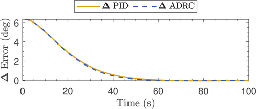
As with the Kuka robot part (Figure 9), an analysis was performed when the robotic system was moved from its ‘home’ state to a point where the rin to be picked up is achievable. From this stage, the error plot (see Figure 6) and the control plot (see Figure 7) were obtained. In this case, it is possible to observe how the error converges to zero at a time close to 55 [sec] when the ADRC control law is applied, while when the traditional PID control law is applied, it does not converge to zero until 60 [sec].

Figure 7. Temporal evolution of the error for the PLMR.

An analysis of the control applied for each DoF of the manipulator was also performed. The corresponding graphs are presented in Figure 8. With them, it is possible to notice that both for the joints that have a change of position in some stage and for those that do not, a lower energy expenditure is required when the ADRC controller is used than when the classical control law is used. This is accentuated in the first 20 s of each stage.

Figure 9. Temporal evolution of the control for each DoF of the Kuka robot.

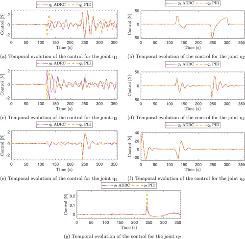
Figure 8. Temporal evolution of the control for the PLMR.

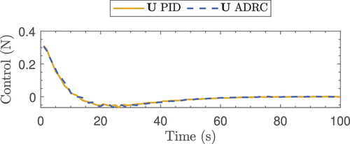
The Mean Square Control (MSC) and Control Integral (CI) per stage, controller, and joint were calculated to confirm the decrease in energy requirement. They are presented in Table 4 and Table 5, respectively.

Table 4. Comparison of the mean square control values for the different control laws at each stage for the Kuka robot.

	Joint MSC
Stage	q1	q2	q3	q4	q6	q7		Total
ST1 - ADRC	5.493${\times }^{-04}$	9.529${\times }^{-05}$	6.831${\times }^{-04}$	3.275${\times }^{-04}$	3.875${\times }^{-05}$	1.123${\times }^{02}$	1.570e-08	1.123${\times }^{02}$
ST1 - PID	4.895${\times }^{-04}$	2.555${\times }^{-04}$	4.892${\times }^{-04}$	4.037${\times }^{-04}$	1.017${\times }^{-04}$	1.124${\times }^{02}$	1.963e-08	1.124${\times }^{02}$
ST2 - ADRC	2.477${\times }^{-01}$	7.711${\times }^{01}$	7.072${\times }^{-01}$	6.472${\times }^{01}$	3.598${\times }^{-02}$	5.435${\times }^{01}$	8.407${\times }^{-06}$	1.972${\times }^{02}$
ST2 - PID	5.568${\times }^{-01}$	7.902${\times }^{01}$	5.841${\times }^{-01}$	7.202${\times }^{01}$	1.406${\times }^{-02}$	5.347${\times }^{01}$	9.859${\times }^{-06}$	2.057${\times }^{02}$
ST3 - ADRC	1.286	2.796${\times }^{02}$	2.272${\times }^{-01}$	1.594${\times }^{02}$	3.462${\times }^{-01}$	3.210${\times }^{-02}$	7.916${\times }^{-04}$	4.410${\times }^{02}$
ST3 - PID	1.516	2.793${\times }^{02}$	1.380${\times }^{-01}$	1.808${\times }^{02}$	5.782${\times }^{-01}$	4.509${\times }^{-02}$	2.814${\times }^{-03}$	4.624${\times }^{02}$

Table 5. Comparison of the control integral values for the different control laws at each stage for the Kuka robot.

	Joint CI
Stage	q1	q2	q3	q4	q6	q7		Total
ST1 - ADRC	1.648${\times }^{-02}$	2.859${\times }^{-03}$	2.049${\times }^{-02}$	9.824${\times }^{-03}$	1.163${\times }^{-03}$	3.369${\times }^{03}$	4.709${\times }^{-07}$	3.369${\times }^{03}$
ST1 - PID	1.468${\times }^{-02}$	7.664${\times }^{-03}$	1.468${\times }^{-02}$	1.211${\times }^{-02}$	3.051${\times }^{-03}$	3.372${\times }^{03}$	5.888${\times }^{-07}$	3.372${\times }^{03}$
ST2 - ADRC	7.430	2.313${\times }^{03}$	2.122${\times }^{01}$	1.942${\times }^{03}$	1.079	1.631${\times }^{03}$	2.522${\times }^{-04}$	5.915${\times }^{03}$
ST2 - PID	1.670${\times }^{01}$	2.370${\times }^{03}$	1.752${\times }^{01}$	2.161${\times }^{03}$	4.218${\times }^{-01}$	1.604${\times }^{03}$	2.958${\times }^{-04}$	6.170${\times }^{03}$
ST3 - ADRC	3.857${\times }^{01}$	8.388${\times }^{03}$	6.815	4.783${\times }^{03}$	1.039${\times }^{01}$	9.629${\times }^{-01}$	2.375${\times }^{-02}$	1.323${\times }^{04}$
ST3 - PID	4.547${\times }^{01}$	8.380${\times }^{03}$	4.139	5.423${\times }^{03}$	1.735${\times }^{01}$	1.353	8.442${\times }^{-02}$	1.387${\times }^{04}$

For the first stage, even though there is an increase of about 0.05% in the error when the system acts under the ADRC law, this law presents a decrease in both the MSC and the CI of about 0.05% compared to the system when it has the PID control law. During the second stage, it can be seen a 4.1% of decrease in CI and MSC when the ADRC controller is used compared to the PID-type controller. Finally, during the third stage, it is possible to observe a better compensation of the manipulator dynamics modification, which is reflected in a decrease of almost 5% in the CI and MSC when using the ADRC controller compared to the PID controller.

The numerical simulations show that ADRC and PID algorithms may exhibit similar error tracking for each DoF. Notice that the comparison of the transient evolution demonstrates the benefit of the ADRC controller showing the tracking error’s convergence, mitigating the change in the manipulator dynamics produced by the task of moving the wheel.

In addition, a significant reduction of the control signal and the tracking error due to ADRC law highlights the improvement enforced with the application of the adaptive form, despite the change in the robot’s dynamics due to the proposed task.

8. Conclusions

This paper introduces a set of successful controllers for robotic manipulators with joint restrictions, employing a novel adaptive gain strategy to address the tracking trajectory problem. The controllers encompass state feedback, output feedback, and a robust version of state feedback that accounts for limited knowledge of manipulator dynamics that can be used in recycling facilities working purely autonomously. All of them utilise state-dependent gains to enforce a better tracking of the reference trajectories. Applying a controlled Lyapunov function establishes the zero trajectory of the tracking error space as asymptotically stable in the Lyapunov sense. Several crucial factors must be considered for the potential implementation of the proposed controller, taking into account processing for the control implementation. Processing speed is a critical consideration for most controllers, but in the case of the proposed controller, higher processing speeds enhance its performance. Therefore, it is imperative to implement this class of controllers on high-speed processors.

Simulated results, incorporating physically inspired joint motion limitations, confirm the satisfaction of the proposed predefined joint motion. Additionally, the efficiency of the proposed adaptive controller enables effective management of external perturbations, as evidenced in the simulated results.

Notably, the presented results affirm the advantages of the adaptive controller compared to similar designs, such as the traditional proportional-integral-derivative control form. Moreover, meeting limitations with an arbitrary structure opens up possibilities for deriving novel alternatives to control complex robotic devices in diverse recycling industries where autonomous manipulators could solve the problem by implementing a hybrid system formulation. The suggested controller can be applied to accomplish more intricate tasks where the robotic device may have complex motion restrictions and velocities.

Acknowledgments

The authors would like to thank the Tecnologico de Monterrey Challenge-Based Research Program project ID IJXT070-22TE60001 and Programa para la Vinculación de Empresas con Instituciones de Educación Superior y Centros de Investigación Comecyt-EdoMex número de proyecto Vinculacion/2023/009.

Disclosure statement

No potential conflict of interest was reported by the author(s).

Data availability statement

The data that support the findings of this study are available from the corresponding author, [author initials], upon reasonable request.

Additional information

Funding

The work was supported by the Instituto Tecnologico de Estudios Superiores de Monterrey, Challenge-Based Research Program [ID IKXT025-22UI60001].

Notes on contributors

Karen Mendoza-Bautista

Karen Mendoza-Bautista received a B.S. degree in biomedical engineering from the National Polytechnic Institute (IPN), Mexico City, Mexico, in 2019 and a master’s degree in Robotics and Advanced Manufacturing, Center of Investigation and Advanced Researching (CINVESTAV) campus Saltillo, IPN, in 2022. Actually, she is studying for a PhD at the Technological Institute of Monterrey (ITESM) in Engineering Sciences. She is also working as a part-time professor on the ITESM campus in Guadalajara. Her current research interests include robot control theory, surgical robots, adaptive control, and vision systems applied to robots. She has published about 3 papers in recognized technical journals.

Mariel Alfaro-Ponce

Mariel Alfaro-Ponce is an assistant professor in the Biomedical Engineering Program at Tecnológico de Monterrey Ciudad de Mexico; she received a bachelor’s degree in Biomedical Engineering, a Master of Science in Microelectronic Engineering, and a Ph.D. in Computer Science from the Instituto Politecnico Nacional, Mexico. Her research interests include artificial intelligence, rehabilitation devices, and intelligent bioinstrumentation. She has been a member of the National System of Researchers of Mexico (SNI-Level I). From 2022 until now, is the head of the Manufacturing Processes for Advanced Materials CDMX research unit.

Isaac Chairez

Isaac Chairez earned the B.S. degree in biomedical engineering from the National Polytechnic Institute (IPN), Mexico City, Mexico, in 2002, and the master’s and Ph.D. degrees from the Department of Automatic Control, Center of Investigation and Advanced Researching (CINVESTAV), IPN, in 2004 and 2007, respectively. He is currently with the National School of Sciences and Engineering of the Tecnológico de Monterrey and the Professional Interdisciplinary Unit of Biotechnology, IPN. He has published over 230 contributions in indexed journals and 300 in international conferences. He has published two books on the applications of neural networks on diverse disciplines. His current research interests include neural networks, fuzzy control theory, nonlinear control, adaptive control, and game theory.

Appendix: Proof of the main theorem

Proof. The application of the proposed controller in (40) over the tracking error dynamics presented in (38) leads to the following equivalent differential equation:

(52) $\begin{array}{c}\frac{d}{\mathit{dt}}{\mathrm{\Delta }}_a(\mathit{t})={\mathrm{\Delta }}_b(\mathit{t}),\\ \frac{d}{\mathit{dt}}{\mathrm{\Delta }}_b(\mathit{t})=W_{\sigma }\left(\mathrm{\Delta }(\mathit{t}|\mathit{k})\right)-\mathit{\eta }\left({\varsigma }_a(\mathit{t}),{\varsigma }_b(\mathit{t}),\mathit{t}\right),\end{array}$(52)

where $W_{\sigma }\left(\mathrm{\Delta }(\mathit{t}|\mathit{k})\right)$ could take the values of $W_1\left({\left.\mathrm{\Delta }\right|}_{\mathit{\sigma }(\mathit{t})=1}(\mathit{t}|\mathit{k})\right)$ or $W_2\left({\left.\mathrm{\Delta }\right|}_{\mathit{\sigma }(\mathit{t})=2}(\mathit{t}|\mathit{k})\right)$ depending on the active scenario.

The substitution of the selected forms for $W_1$ and $W_2$ in (41) implies the following equivalent dynamics:

(53) $\begin{array}{c}\frac{d}{\mathit{dt}}{\mathrm{\Delta }}_{\alpha }\left(\mathit{t}\right)={\mathrm{\Delta }}_{\beta }\left(\mathit{t}\right)\\ \frac{d}{\mathit{dt}}{\mathrm{\Delta }}_{\beta }\left(\mathit{t}\right)={\mathrm{\Delta }}_a\left(\mathit{t}\right)\\ \frac{d}{\mathit{dt}}{\mathrm{\Delta }}_a\left(\mathit{t}\right)={\mathrm{\Delta }}_b\left(\mathit{t}\right)\\ \frac{d}{\mathit{dt}}{\mathrm{\Delta }}_b\left(\mathit{t}\right)=K_{\mathit{P},\mathit{\sigma }}(\mathit{t}|\mathit{k}){\mathrm{\Delta }}_a\left(\mathit{t}\right)+K_{\mathit{D},\mathit{\sigma }}(\mathit{t}|\mathit{k}){\mathrm{\Delta }}_b\left(\mathit{t}\right)+\setminus \mathit{cr}{K}_{\mathit{I},\mathit{\sigma }}(\mathit{t}|\mathit{k}){\mathrm{\Delta }}_{\beta }\left(\mathit{t}\right)+K_{\mathit{II},\mathit{\sigma }}(\mathit{t}|\mathit{k}){\mathrm{\Delta }}_{\alpha }\left(\mathit{t}\right)-\mathit{\eta }\left({\varsigma }_a\left(\mathit{t}\right),{\varsigma }_b\left(\mathit{t}\right),\mathit{t}\right).\end{array}$(53)

This differential equation is valid with $K_{\mathit{II},1}(\mathit{t}|\mathit{k})\equiv 0,\mathrm{\forall t}\ge 0$.

The expression presented in (53) is equivalent to (using the expressions of ${\tilde{K}}_{\mathit{P},\mathit{\sigma }}(\mathit{t}|\mathit{k})$, ${\tilde{K}}_{\mathit{D},\mathit{\sigma }}(\mathit{t}|\mathit{k})$, ${\tilde{K}}_{\mathit{I},\mathit{\sigma }}(\mathit{t}|\mathit{k})$, and ${\tilde{K}}_{\mathit{II},\mathit{\sigma }}(\mathit{t}|\mathit{k})$) to the following differential form with ${\mathrm{\Delta }}^{\mathrm{T}}=\left[{{\mathrm{\Delta }}_{\alpha }}^{\mathrm{T}},{{\mathrm{\Delta }}_{\beta }}^{\mathrm{T}},{{\mathrm{\Delta }}_a}^{\mathrm{T}},{{\mathrm{\Delta }}_b}^{\mathrm{T}}\right]$:

(54) $\frac{d}{\mathit{dt}}\mathrm{\Delta }\left(\mathit{t}\right)=\left(\mathbf{A}\left(\mathit{k}\right)+{\mathbf{B}\mathbf{K}}_{\sigma }^{\ast }\left(\mathit{k}\right)\right)\mathrm{\Delta }\left(\mathit{t}\right)-\mathbf{B}\mathit{\eta }\left({\varsigma }_a\left(\mathit{t}\right),{\varsigma }_b\left(\mathit{t}\right),\mathit{t}\right)+\mathbf{B}{\tilde{\mathbf{K}}}_{\mathit{\sigma }}(\mathit{t}|\mathit{k})\mathrm{\Delta }\left(\mathit{t}\right),$(54)

here ${\tilde{K}}_{\mathit{II},\mathit{\sigma }}(\mathit{t}|\mathit{k})=K_{\mathit{II},\mathit{\sigma }}(\mathit{t}|\mathit{k})-K_{II}^{\ast }(\mathit{k})$, ${\tilde{K}}_{\mathit{I},\mathit{\sigma }}(\mathit{t}|\mathit{k})=K_{\mathit{I},\mathit{\sigma }}(\mathit{t}|\mathit{k})-K_I^{\ast }(\mathit{k})$, ${\tilde{K}}_{\mathit{D},\mathit{\sigma }}(\mathit{t}|\mathit{k})=K_{\mathit{D},\mathit{\sigma }}(\mathit{t}|\mathit{k})-K_D^{\ast }(\mathit{k})$, and ${\tilde{K}}_{\mathit{P},\mathit{\sigma }}(\mathit{t}|\mathit{k})=K_{\mathit{P},\mathit{\sigma }}(\mathit{t}|\mathit{k})-K_P^{\ast }(\mathit{k})$.

Consider the mixed Lyapunov candidate function (valid for each domain for continuous time and that we can analyse after each scenario change) given by:

(55) $\begin{array}{c}{V}_1\left(\mathrm{\Delta }(\mathit{t}),{\tilde{\mathbf{K}}}_{\mathit{\sigma }}(\mathit{t}|\mathit{k})\right)={\mathrm{\Delta }}^{\mathrm{T}}(\mathit{t})\mathit{P}(\mathit{k})\mathrm{\Delta }(\mathit{t})+\mathrm{tr}\left\{{\tilde{\mathbf{K}}}_{\mathit{\sigma }}^{\mathrm{T}}(\mathit{t}|\mathit{k}){\mathrm{\Lambda }}_C^{-1}{\tilde{\mathbf{K}}}_{\mathit{\sigma }}(\mathit{t}|\mathit{k})\right\},\\ V_2\left(\mathrm{\Delta }(t_k),{\tilde{\mathbf{K}}}_{\mathit{\sigma }}(t_k|\mathit{k})\right)={\mathrm{\Delta }}^{\mathrm{T}}(t_k)\mathit{P}(\mathit{k})\mathrm{\Delta }(t_k)+\mathrm{tr}\left\{{\tilde{\mathbf{K}}}_{\mathit{\sigma }}^{\mathrm{T}}(t_k|\mathit{k}){\mathrm{\Lambda }}_D^{-1}{\tilde{\mathbf{K}}}_{\mathit{\sigma }}(t_k|\mathit{k})\right\},\end{array}$(55)

here we keep the notation $\mathrm{\Delta }(\mathit{t})$ in the definition of the function $V_1$ to emphasise the continuous-time analysis. In contrast, in the case of $V_2$, we considered the values of $\mathit{t}=t_k$ corresponding to the moments corresponding to the change of scenario.

The time derivative of the first function in (55), $V_1\left(\mathrm{\Delta }(\mathit{t}),{\tilde{\mathbf{K}}}_{\mathit{\sigma }}(\mathit{t}|\mathit{k})\right)$, that is

(56) $\frac{d}{\mathit{dt}}{V}_1\left(\mathrm{\Delta }\left(\mathit{t}\right),{\tilde{\mathbf{K}}}_{\mathit{\sigma }}(\mathit{t}|\mathit{k})\right)=2{\mathrm{\Delta }}^{\mathrm{T}}\left(\mathit{t}\right)\mathit{P}\left(\mathit{k}\right)\frac{d}{\mathit{dt}}\mathrm{\Delta }\left(\mathit{t}\right)+2\mathrm{tr}\left\{{\tilde{\mathbf{K}}}_{\mathit{\sigma }}^{\mathrm{T}}(\mathit{t}|\mathit{k}){\mathrm{\Lambda }}_C^{-1}\frac{d}{\mathit{dt}}{\tilde{\mathbf{K}}}_{\mathit{\sigma }}(\mathit{t}|\mathit{k})\right\},$(56)

The substitution of the dynamics corresponding to $\mathrm{\Delta }(\mathit{t})$ in the derivative of $V_1\left(\mathrm{\Delta }(\mathit{t}),{\tilde{\mathbf{K}}}_{\mathit{\sigma }}(\mathit{t}|\mathit{k})\right)$ leads to:

(57) $\begin{array}{c}\frac{d}{\mathit{dt}}{V}_1\left(\mathrm{\Delta }\left(\mathit{t}\right),{\tilde{\mathbf{K}}}_{\mathit{\sigma }}(\mathit{t}|\mathit{k})\right)=\\ 2{\mathrm{\Delta }}^{\mathrm{T}}\left(\mathit{t}\right)\mathit{P}\left(\mathit{k}\right)\left(\left(\mathbf{A}\left(\mathit{k}\right)+{\mathbf{B}\mathbf{K}}_{\sigma }^{\ast }\left(\mathit{k}\right)\right)\mathrm{\Delta }\left(\mathit{t}\right)-\mathbf{B}\mathit{\eta }\left({\varsigma }_a\left(\mathit{t}\right),{\varsigma }_b\left(\mathit{t}\right),\mathit{t}\right)+\mathbf{B}{\tilde{\mathbf{K}}}_{\mathit{\sigma }}(\mathit{t}|\mathit{k})\mathrm{\Delta }\left(\mathit{t}\right)\right)+\\ 2\mathit{tr}\left\{{\tilde{\mathbf{K}}}_{\mathit{\sigma }}^{\mathrm{T}}(\mathit{t}|\mathit{k}){\mathrm{\Lambda }}_C^{-1}\frac{d}{\mathit{dt}}{\tilde{\mathbf{K}}}_{\mathit{\sigma }}(\mathit{t}|\mathit{k})\right\}\end{array}$(57)

The application of a symmetrisation operator and the relationship between the inner product and the trace operator has the following upper estimation for the time derivative of $V_1\left(\mathrm{\Delta }(\mathit{t}),{\tilde{\mathbf{K}}}_{\mathit{\sigma }}(\mathit{t}|\mathit{k})\right)$

(58) $\begin{array}{c}\frac{d}{\mathit{dt}}{V}_1\left(\mathrm{\Delta }\left(\mathit{t}\right),{\tilde{\mathbf{K}}}_{\mathit{\sigma }}(\mathit{t}|\mathit{k})\right)=\\ 2{\mathrm{\Delta }}^{\mathrm{T}}\left(\mathit{t}\right)\mathit{P}\left(\mathit{k}\right)\left(\left(\mathbf{A}\left(\mathit{k}\right)+{\mathbf{B}\mathbf{K}}_{\sigma }^{\ast }\left(\mathit{k}\right)\right)\mathrm{\Delta }\left(\mathit{t}\right)-\mathbf{B}\mathit{\eta }\left({\varsigma }_a\left(\mathit{t}\right),{\varsigma }_b\left(\mathit{t}\right),\mathit{t}\right)+\mathbf{B}{\tilde{\mathbf{K}}}_{\mathit{\sigma }}(\mathit{t}|\mathit{k})\mathrm{\Delta }\left(\mathit{t}\right)\right)+\\ 2\mathit{tr}\left\{{\tilde{\mathbf{K}}}_{\mathit{\sigma }}^{\mathrm{T}}(\mathit{t}|\mathit{k}){\mathrm{\Lambda }}_C^{-1}\frac{d}{\mathit{dt}}{\tilde{\mathbf{K}}}_{\mathit{\sigma }}(\mathit{t}|\mathit{k})\right\}\end{array}$(58)

The previous differential inclusion was obtained after applying the so-called lambda inequality $X^{\mathrm{T}}\mathit{Y}+Y^{\mathrm{T}}\mathit{X}\le X^{\mathrm{T}}{\mathrm{\Sigma }}^{-1}\mathit{X}+Y^{\mathrm{T}}\mathrm{\Sigma }\mathit{Y}$, $\mathit{X}$$\mathit{Y}\in {\mathbb{R}}^{\mathit{\rho }\times \mathit{l}}$ with $0<\mathrm{\Lambda }={\mathrm{\Lambda }}^{\mathrm{T}}\in {\mathbb{R}}^{\mathit{\rho }\times \mathit{\rho }}$ (Poznyak 2008).

Taking the assumption on the existence of positive definite solutions for the Riccati equation depending on $P_1$ and $P_2$ presented in the Theorem description and considering the class of adjustment methods for the gains $K_{\mathit{II},\mathit{\sigma }}(\mathit{t}|\mathit{k})$, $K_{\mathit{I},\mathit{\sigma }}(\mathit{t}|\mathit{k})$, $K_{\mathit{D},\mathit{\sigma }}(\mathit{t}|\mathit{k})$, and $K_{\mathit{P},\mathit{\sigma }}(\mathit{t}|\mathit{k})$, (all of them included in $K_{\sigma }(\mathit{t}|\mathit{k})$) presented in (42), one gets that last inclusion can be transformed to: $\frac{d}{\mathit{dt}}{V}_1\left(\mathrm{\Delta }\left(\mathit{t}\right),{\tilde{\mathbf{K}}}_{\mathit{\sigma }}(\mathit{t}|\mathit{k})\right)\le -{\alpha }_{Q_C}\frac{d}{\mathit{dt}}{V}_1\left(\mathrm{\Delta }\left(\mathit{t}\right),{\tilde{\mathbf{K}}}_{\mathit{\sigma }}(\mathit{t}|\mathit{k})\right)+{\lambda }_{\mathit{max}}\left\{{\mathrm{\Sigma }}_1\right\}{\eta }_0$.

The estimation of the integral operator applied to the previous inclusion, and by the comparison Lemma, it can be proven that $V_1\left(\mathrm{\Delta }\left(\mathit{t}\right),{\tilde{\mathbf{K}}}_{\mathit{\sigma }}(\mathit{t}|\mathit{k})\right)\le V_1\left(\mathrm{\Delta }\left(t_{\mathit{k}-1}\right),{\tilde{\mathbf{K}}}_{\mathit{\sigma }}{(}_{\mathit{k}-1}|\mathit{k})\right)e^{-{\alpha }_{Q_C}\left(\mathit{t}-t_{\mathit{k}-1}\right)}+\frac{{\mathit{\lambda }}_{\mathit{max}}\left\{{\mathrm{\Sigma }}_1\right\}{\eta }_0}{{\alpha }_{Q_C}}\left(1-e^{-\alpha \left(t-\left(T_i+T_e\right)\right)}\right)$, which is valid $\mathrm{\forall t}\in [t_{\mathit{k}-1},t_k)$. Notice that this analysis is valid within each scenario where the continuous dynamics is valid.

Considering the structure of the proposed continuous form of the Lyapunov-like equation, one may confirm that $\mathrm{\forall t}\in [t_{\mathit{k}-1},t_k)$ the following inequality is valid

(59) $\begin{array}{c}||\mathrm{\Delta }\left(\mathit{t}\right)|{|}^2\le \frac{V_1\left(\mathrm{\Delta }\left(t_{\mathit{k}-1}\right),{\tilde{\mathbf{K}}}_{\mathit{\sigma }}{(}_{\mathit{k}-1}|\mathit{k})\right)}{{\lambda }_{\mathit{min}}\left\{\mathit{P}\left(\mathit{k}\right)\right\}}{e}^{-{\alpha }_{Q_C}\left(\mathit{t}-t_{\mathit{k}-1}\right)}+\\ \frac{{\mathit{\lambda }}_{\mathit{max}}\left\{{\mathrm{\Sigma }}_1\right\}{\eta }_0}{{\lambda }_{\mathit{min}}\left\{\mathit{P}\left(\mathit{k}\right)\right\}{\alpha }_{Q_C}}\left(1-e^{-\alpha \left(t-\left(T_i+T_e\right)\right)}\right)\\ \mathit{\hspace{0.17em}}\end{array}$(59)

Now, taking into consideration the evolution of matrix $\mathit{P}(\mathit{k})$ for the $\mathit{k}-\mathit{th}$ object to be handled, consider the study of the candidate Lyapunov function $V_2\left(\mathrm{\Delta }(t_k),{\tilde{\mathbf{K}}}_{\mathit{\sigma }}(t_k|\mathit{k})\right)$ in discrete sense.

The second part of the proof will take advantage of the explicit discretisation applied to the dynamics of the tracking error $\mathrm{\Delta }$, implying that (54) can be presented as follows:

(60) $\begin{array}{c}\mathrm{\Delta }(t_k)-\mathrm{\Delta }(t_{\mathit{k}-1})={\mathrm{\Pi }}_{\mathit{k}-1}\left(\mathbf{A}(\mathit{k})+{\mathbf{B}\mathbf{K}}_{\sigma }^{\ast }(\mathit{k})\right)\mathrm{\Delta }(t_{\mathit{k}-1})-\\ {\mathrm{\Pi }}_{\mathit{k}-1}\mathbf{B}\mathit{\eta }\left({\varsigma }_a(\mathit{t}),{\varsigma }_b(\mathit{t}),\mathit{t}\right)+{\mathrm{\Pi }}_{\mathit{k}-1}\mathbf{B}{\tilde{\mathbf{K}}}_{\mathit{\sigma }}(t_{\mathit{k}-1}|\mathit{k})\mathrm{\Delta }(t_{\mathit{k}-1})\end{array}$(60)

From the expression (60), we may estimate that

(61) $\begin{array}{c}\mathrm{\Delta }(t_k)=\mathrm{{\rm Y}}(t_{\mathit{k}-1}|\mathit{k})\mathrm{\Delta }(t_{\mathit{k}-1})-{\mathrm{\Pi }}_{\mathit{k}-1}\mathbf{B}\mathit{\eta }\left({\varsigma }_a(\mathit{t}),{\varsigma }_b(\mathit{t}),\mathit{t}\right)\end{array}$(61)

Now, using these discrete dynamics on the candidate Lyapunov function $V_2\left(\mathrm{\Delta }(t_k),{\tilde{\mathbf{K}}}_{\mathit{\sigma }}(t_k|\mathit{k})\right)$, one has to estimate the variation of such function at two consecutive times when the scenario changes $\mathrm{\Delta }{V}_2\left(\mathrm{\Delta }(t_k),{\tilde{\mathbf{K}}}_{\mathit{\sigma }}(t_k|\mathit{k})\right)=V_2\left(\mathrm{\Delta }(t_k),{\tilde{\mathbf{K}}}_{\mathit{\sigma }}(t_k|\mathit{k})\right)-V_2\left(\mathrm{\Delta }(t_{\mathit{k}-1}),{\tilde{\mathbf{K}}}_{\mathit{\sigma }}(t_{\mathit{k}-1}|\mathit{k})\right)$

(62) $\begin{array}{c}\mathrm{\Delta }{V}_2\left(\mathrm{\Delta }(t_k),{\tilde{\mathbf{K}}}_{\mathit{\sigma }}(t_k|\mathit{k})\right)={\mathrm{\Delta }}^{\mathrm{T}}(t_k)\mathit{P}(\mathit{k})\mathrm{\Delta }(t_k)-{\mathrm{\Delta }}^{\mathrm{T}}(t_{\mathit{k}-1})\mathit{P}(\mathit{k})\mathrm{\Delta }(t_{\mathit{k}-1}).\end{array}$(62)

This function is proposed considering that there are no jumps on the gains on the boundary between scenarios. Then, based on the proposed Lyapunov candidate function, one has the following estimate considering the discrete dynamics (61):

(63) $\begin{array}{c}\mathrm{\Delta }{V}_2\left(\mathrm{\Delta }(t_k),{\tilde{\mathbf{K}}}_{\mathit{\sigma }}(t_k|\mathit{k})\right)\le \\ {\mathrm{\Delta }}^{\mathrm{T}}(t_{\mathit{k}-1})\left[{\mathrm{{\rm Y}}}^{\mathrm{T}}(t_{\mathit{k}-1}|\mathit{k})\left(\mathit{P}(\mathit{k})+\mathrm{\Omega }\right)\mathrm{{\rm Y}}(t_{\mathit{k}-1}|\mathit{k})-\mathit{P}(\mathit{k})\right]\mathrm{\Delta }(t_{\mathit{k}-1})+\\ \\ {\mathrm{\Pi }}_{k-1}^2{\eta }^{\mathrm{T}}\left({\varsigma }_a(\mathit{t}),{\varsigma }_b(\mathit{t}),\mathit{t}\right){\mathbf{B}}^{\mathrm{T}}\left(\mathit{I}+{\mathrm{\Omega }}^{-1}\right)\mathbf{B}\mathit{\eta }\left({\varsigma }_a(\mathit{t}),{\varsigma }_b(\mathit{t}),\mathit{t}\right)\end{array}$(63)

Using the Rayleigh inequality and the upper bound for the admissible class of external uncertainties and modelling imprecision, the following upper bound is valid

(64) $\begin{array}{c}\mathrm{\Delta }{V}_2\left(\mathrm{\Delta }(t_k),{\tilde{\mathbf{K}}}_{\mathit{\sigma }}(t_k|\mathit{k})\right)\le {\mathrm{\Pi }}_{k-1}^2{\lambda }_{\mathit{max}}\left\{{\mathbf{B}}^{\mathrm{T}}\left(\mathit{I}+{\mathrm{\Omega }}^{-1}\right)\mathbf{B}\right\}{\eta }_0+\\ {\mathrm{\Delta }}^{\mathrm{T}}(t_{\mathit{k}-1})\left[{\mathrm{{\rm Y}}}^{\mathrm{T}}(t_{\mathit{k}-1}|\mathit{k})\left(\mathit{P}(\mathit{k})+\mathrm{\Omega }\right)\mathrm{{\rm Y}}(t_{\mathit{k}-1}|\mathit{k})-\mathit{P}(\mathit{k})\right]\mathrm{\Delta }(t_{\mathit{k}-1})\end{array}$(64)

Taking the assumption on the existence of positive definite solutions for the discrete Riccati equation establishing the evolution of matrix $\mathit{P}(\mathit{k})$ at each change of scenario leads to

(65) $\begin{array}{c}\mathrm{\Delta }{V}_2\left(\mathrm{\Delta }(t_k),{\tilde{\mathbf{K}}}_{\mathit{\sigma }}(t_k|\mathit{k})\right)\le {\mathrm{\Pi }}_{k-1}^2{\lambda }_{\mathit{max}}\left\{{\mathbf{B}}^{\mathrm{T}}\left(\mathit{I}+{\mathrm{\Omega }}^{-1}\right)\mathbf{B}\right\}{\eta }_0-{\mathrm{\Delta }}^{\mathrm{T}}(t_{\mathit{k}-1})Q_D(\mathit{k})\mathrm{\Delta }(t_{\mathit{k}-1})\end{array}$(65)

Hence, one may notice that $\mathrm{\Delta }{V}_2\left(\mathrm{\Delta }(t_k),{\tilde{\mathbf{K}}}_{\mathit{\sigma }}(t_k|\mathit{k})\right)<0$ if ${\mathrm{\Pi }}_{k-1}^2{\lambda }_{\mathit{max}}\left\{{\mathbf{B}}^{\mathrm{T}}\left(\mathit{I}+{\mathrm{\Omega }}^{-1}\right)\mathbf{B}\right\}{\eta }_0\le {\mathrm{\Delta }}^{\mathrm{T}}(t_{\mathit{k}-1})Q_D(\mathit{k})\mathrm{\Delta }(t_{\mathit{k}-1})$

This last result completes the proof.

References

- Ames, A. D., E. A. Cousineau, and M. J. Powell 2012. “Dynamically Stable Bipedal Robotic Walking with Nao via Human-Inspired Hybrid Zero Dynamics”. Proceedings of the 15th acm international conference on hybrid systems: Computation and control, Beijin, China, April 17–19, 135–144.
- Branicky, M. S., V. S. Borkar, and S. K. Mitter 1994. “A Unified Framework for Hybrid Control”. Proceedings of 1994 33rd IEEE Conference on Decision and Control, Lake Buena Vista, FL, USA, December 14–16.
- Capuzzi, S., and G. Timelli. 2018. “Preparation and Melting of Scrap in Aluminum Recycling: A Review.” Metals 8 (4): 249. https://doi.org/10.3390/met8040249.
- Crampin, M. 1981. “On the Differential Geometry of the Euler-Lagrange Equations, and the Inverse Problem of Lagrangian Dynamics.” Journal of Physics A: Mathematical and General 14 (10): 2567. https://doi.org/10.1088/0305-4470/14/10/012.
- Cruz, D., A. Luviano-Juárez, and I. Chairez. 2014. Output sliding mode controller to regulate the gait of Gecko-inspired robot. Memorias del XVI Congreso Latinoamericano de Control Automático, CLCA, Cancún, Quintana Roo, México, Ocotober 14–17. Mexico City.
- Ezeah, C., J. A. Fazakerley, and C. L. Roberts. 2013. “Emerging Trends in Informal Sector Recycling in Developing and Transition Countries.” Waste Management 33 (11): 2509–2519. https://doi.org/10.1016/j.wasman.2013.06.020.
- Grimaud, G., N. Perry, and B. Laratte. 2016. “Life Cycle Assessment of Aluminium Recycling Process: Case of Shredder Cables.” Procedia Cirp 48:212–218. https://doi.org/10.1016/j.procir.2016.03.097.
- Koutsoukos, X. D., P. J. Antsaklis, J. A. Stiver, and M. D. Lemmon. 2000. “Supervisory Control of Hybrid Systems.” Proceedings of the IEEE 88 (7): 1026–1049. https://doi.org/10.1109/5.871307.
- Lennartson, B., M. Tittus, B. Egardt, and S. Pettersson. 1996. “Hybrid Systems in Process Control.” IEEE Control Systems Magazine 16 (5): 45–56.
- Levant, A. 1998. “Robust exact differentiation via sliding mode technique.” Automatica 34 (3): 379–384. https://doi.org/10.1016/S0005-1098(97)00209-4.
- Lu, Y., B. Yang, Y. Gao, and Z. Xu. 2022. “An Automatic Sorting System for Electronic Components Detached from Waste Printed Circuit Boards.” Waste Management 137:1–8. https://doi.org/10.1016/j.wasman.2021.10.016.
- Ordaz, P., and A. Poznyak. 2015a. “‘Kl’-Gain Adaptation for Attractive Ellipsoid Method.” IMA Journal of Mathematical Control and Information 32 (3): 447–469. https://doi.org/10.1093/imamci/dnt046.
- Ordaz, P., and A. Poznyak. 2015b. “‘Kl’-Gain Adaptation for Attractive Ellipsoid Method.” IMA Journal of Mathematical Control and Information 32 (3): 447–469. https://doi.org/10.1093/imamci/dnt046.
- Ortega, R., A. Loria, R. Kelly, and L. Praly 1994. “On Passivity-Based Output Feedback Global Stabilization of Euler-Lagrange Systems”. Proceedings of 1994 33rd IEEE Conference on Decision and Control, Lake Buena Vista, FL, USA, December 14–16. https://doi.org/10.1109/CDC.1994.410898.
- Polyakov, A. 2010. “Invariant Ellipsoid Method for Time-Delayed Predictor-Based Sliding Mode Control System”. 2010 11th International Workshop on Variable Structure Systems (VSS), Mexico City, Mexico, June 26–28. https://doi.org/10.1109/VSS.2010.5544685.
- Polyakov, A., and A. Poznyak 2009. “Minimization of the Unmatched Disturbances in the Sliding Mode Control Systems via Invariant Ellipsoid Method”. 2009 ieee control applications,(cca) & intelligent control,(isic), St. Petersburg, Russia, July 08–10. https://doi.org/10.1109/CCA.2009.5280842.
- Poznyak, A. 2008. Advanced Mathematical Tools for Automatic Control Engineers: Volume 1: Deterministic Systems, 775. Amsterdam: Elsevier Science.
- Schlesinger, M. E. 2006. Aluminum recycling, 248. Boca Raton, Fl, USA: CRC press.
- Schmitz, C. 2006. Handbook of Aluminium Recycling, 454. Essen, Germany: Vulkan-Verlag GmbH.
- Shinzato, M. C., and R. Hypolito. 2005. “Solid Waste from Aluminum Recycling Process: Characterization and Reuse of Its Economically Valuable Constituents.” Waste Management 25 (1): 37–46. https://doi.org/10.1016/j.wasman.2004.08.005.
- Spong, M. W., and M. Vidyasagar. 1989. Robot Dynamics and Control, wa343. New York, USA: John Wiley & Sons.
- Yoshikawa, T., and A. Sudou. 1993. “Dynamic Hybrid Position/Force Control of Robot Manipulators-On-Line Estimation of Unknown Constraint.” IEEE Transactions on Robotics and Automation 9 (2): 220–226. https://doi.org/10.1109/70.238286.