Spatially Clustered Movement Patterns and Segregation of Subadult Chinook Salmon within the Salish Sea

Abstract

While Pacific salmon are known for their extensive marine migrations, some species display much more limited alternative patterns, including residence within interior marine waters. To more clearly define the scale of movement of these residents, we used acoustic telemetry to track subadult Chinook Salmon Oncorhynchus tshawytscha caught in and released from discrete areas of the Salish Sea. Their movements were determined from detections at fixed receivers in central Puget Sound, Admiralty Inlet, the San Juan Islands, and the Strait of Juan de Fuca. Cluster analysis of the detections indicated four groups, with much less commonality of movement than might be inferred from the proximity of the tagging locations, which were only tens of kilometers apart. For example, none of the salmon tagged in central Puget Sound were detected in the San Juan Islands and vice versa. Thus, Chinook Salmon occupying central Puget Sound and the San Juan Islands may exhibit different distributions, extents of movement, and degrees of basin fidelity. These results provide information relevant to the management and conservation of this species, which is listed as threatened under the U.S. Endangered Species Act, and whose movements cross the U.S.–Canadian boundary. These findings may also help explain the variation in organic contaminant levels among Puget Sound-origin Chinook Salmon.

Received June 24, 2016; accepted October 4, 2016

Migratory behavior is widely distributed among animal taxa, playing a central role in their ecology, evolution (Baker 1978; Dingle 1996), and population dynamics (Morales et al. 2010). Migration plays an important role in ecosystem processes and conservation because it can link habitats with the transfer of nutrients, disease, and contaminants (Bauer and Hoye 2014). Among fishes, Atlantic and Pacific salmon are famous for the great distances that they travel at sea and upriver. However, these species also display a wide range of migratory patterns, including nonanadromous populations and nonanadromous individuals within largely anadromous populations (reviewed by Quinn 2005; Jonsson and Jonsson 2011). Moreover, anadromous individuals may vary greatly in their use of marine habitats. For example, Chinook Salmon Oncorhynchus tshawytscha forage in both distant oceanic regions and coastal waters (Waples et al. 2004; Sharma and Quinn 2012) and also occupy interior marine water bodies such as the Salish Sea, spanning southern British Columbia, Canada, and Washington State (Pressay 1953; Haw et al. 1967; O’Neill and West 2009; Chamberlin et al. 2011a). The intraspecific variation in marine migrations is not only an interesting aspect of their behavioral ecology, but the political boundaries that the fish cross affect the federal, state, local, and tribal authorities responsible for their management and conservation.

The migration pathways and foraging areas of salmon determine their uptake of chemical contaminants. Salmon that are resident in Puget Sound are part of a food web that is markedly higher in persistent organic contaminants than the Strait of Georgia, farther north in the Salish Sea, and along the Pacific Ocean coast, as revealed by contaminant levels in forage fish species that are prey of the Chinook Salmon (West et al. 2008) and other predators (Good et al. 2014). Chinook Salmon that are resident in Puget Sound have much higher levels of these contaminants than salmon feeding along the coast (O’Neill et al. 1998; O’Neill and West 2009), with implications for the health of marine mammals (Cullon et al. 2005, 2009) and humans (Washington State Department of Health 2006) that regularly consume them.

Residents constitute a significant fraction of all Puget Sound Chinook Salmon (O’Neill and West 2009), are part of breeding populations from all regions of Puget Sound (Chamberlin et al. 2011a, 2011b), and are also found in Canadian waters of the Salish Sea (Healey and Groot 1987). Partial migration is a common life history trait and widespread alternative to the better studied coastal and ocean migration patterns. Chinook Salmon marked as juveniles with coded wire tags were more often recovered in their natal region of Puget Sound than would occur by chance, but considerable exchange among regions was observed (Chamberlin et al. 2011a). Coded wire tag recoveries (Chamberlin et al. 2011a; Chamberlin and Quinn 2014) and a fishery regulation assessment model (O’Neill and West 2009) indicated that approximately 70% of the juveniles from a given population might migrate to the coast and the other ca. 30% might stay in Puget Sound as residents, although these proportions varied for hatchery-produced Chinook Salmon by size and age at release and the year and region of release.

Initial telemetry studies of residents (subadult Chinook Salmon captured in Puget Sound during the winter and spring, when members of their cohort would otherwise be found along the Pacific Ocean coast or offshore waters: Trudel et al. 2009) indicated that some remained in a limited geographic area, but a few later left Puget Sound (A. N. Kagley and coworkers, unpublished). However, all of the Chinook Salmon in that study were tagged in central Puget Sound (CPS), so the movements could not be compared with those of salmon from other regions. In addition, there were no receivers in the San Juan Islands (SJI), an archipelago in northern Puget Sound long known to fishermen and fisheries managers as a feeding area for resident Chinook Salmon.

The goal of this study was to investigate the movements of subadult Chinook Salmon within the Salish Sea. Specifically, we tagged salmon in three proximate areas in the CPS, Admiralty Inlet (ADM), and SJI, and detected their movements on a series of fixed receivers. The null hypothesis was that while the number of salmon and duration of detections might vary among receivers, the fish tagged in different areas would be equally represented, relative to the fish from other areas. Alternatively, we predicted that the patterns of detections would be biased by the tagging locations and that the salmon would be more often detected in the region where they had been tagged. This result would be consistent with the coded-wire-tagging records, indicating that local movements of resident salmon tend to be limited, despite the open access to suitable habitats elsewhere, as inferred from their occupancy by salmon from other regions (Chamberlin and Quinn 2014).

Methods

Study site and receiver coverage

Throughout the study period, acoustic receivers, capable of detecting the time of detection and the unique identity of the transmitter surgically implanted inside each fish, were deployed throughout the Salish Sea and Strait of Georgia by a variety of agencies. These receivers were deployed in four regions, including the SJI, Strait of Juan de Fuca (JDF), ADM, and CPS (Figure 1). Receiver arrays across the JDF and ADM had spacing designed to maximize the probability of detecting a fish passing through those water bodies (Moore et al. 2015). The JDF array had two lines 0.3 km apart with 30 receivers each, spaced every 0.8 km and placed approximately 5 m from the bottom at depths of ~10–195 m (Figure 2). The JDF region also had two more individual receivers ca. 15 and 60 km beyond the array in the middle and at the end of the JDF, respectively. The ADM array had a line of 13 receivers spaced every 0.4 km in water approximately 8–145 m deep (Figure 2), and an additional receiver was deployed south of Admiralty Head, Whidbey Island. Sixteen receivers were deployed in the SJI near shore in water averaging 9 m deep at mean low tide. Finally, there were nine receivers in CPS placed 0.2–2.5 km from shore in water 8–230 m deep.

Figure 1. Study area map indicating the three tagging basins (outlined in dashed circles): San Juan Islands, Admiralty Inlet, and central Puget Sound. Tagging areas within basins (gray boxes), the receivers with detections (closed circles), and receivers without detections (x) are indicated.

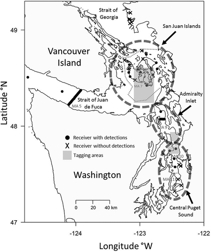
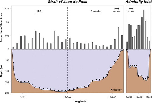
Figure 2. The proportion of detections by resident Chinook Salmon at each receiver in the acoustic arrays at the Strait of Juan de Fuca (JDF) and Admiralty Inlet (ADM) relative to the local bathymetry. Each grey bar represents a matched receiver pair at the JDF dual parallel array (30 pairs) and a single receiver at the ADM one-line array (13 individuals). Receiver positions are aligned, by longitude, with the bathymetric profile (Ryan et al. 2009; http://www.marine-geo.org/tools/GMRTMapTool/) beneath each array. The bathymetric profiles include the location and depth of the receivers, approximately 5 m above the bottom, which correspond to the grey bar above. The dashed vertical line in the JDF panels marks the international boundary between the United States and Canada. The widths of the panels are proportional to the shore-to-shore distance along each array (JDF = 22.80 km, ADM = 5.36 km). The distance between receivers is 0.8 and 0.4 km at the JDF and ADM arrays, respectively.

Receiver downloads were managed through the Puget Sound’s Hydrophone Data Repository (Hydra; http://hydra3.sound-data.com/about/) and Ocean Tracking Network (OTN; http://oceantrackingnetwork.org) of Dalhousie University, Nova Scotia, Canada. Both are online databases allowing a network of researchers to share tag codes, receiver locations, and detection data. We defined the four receiver zones by the marine areas (MA) as delineated for management of local fisheries by the Washington Department of Fish and Wildlife (WDFW) and the Canadian Department of Fisheries and Oceans (DFO): SJI, WDFW MA 7; JDF, WDFW MA 5–DFO MA 20–4; ADM, WDFW MA 9; CPS, WDFW MA 10 and 11 (WDFW 2016; DFO 2016; Figure 1). The JDF array, ADM array, CPS receivers, and three SJI receivers were deployed prior to January 5, 2011, the date of the first detection, and 13 more SJI receivers were activated in November 2011. The SJI receivers were retrieved on October 14, 2013, which defined the end of the study to avoid uneven coverage among areas.

Field methods

A total of 82 Chinook Salmon (FL range = 194 to 600 mm) were captured using hook-and-line fishing techniques between January 5, 2011, and May 17, 2013. Fish were captured in three major basins within the Salish Sea, including the CPS (n = 15, FL = 194 to 345 mm), ADM (n = 23, FL = 250 to 600 mm), and SJI (n = 44, FL = 280 to 545 mm; Figure 1). Fish were captured within the January to June period and would therefore be considered residents of the Salish Sea (Chamberlin et al. 2011a). After capture, fish were transferred to a live well containing aerated flow-through seawater. Fish with visible distress or more than 10% scale loss were not tagged; others were transferred to a small cooler with the anesthetic tricaine methanesulfonate (MS-222) at a concentration of 65 mg/L to induce loss of equilibrium while maintaining opercular movement. Once a fish was adequately sedated, it was weighed and FL was measured to the nearest millimeter. The fish was then transferred to a surgical table on a closed-cell foam with a cutout that allowed the individual to be positioned on its dorsal side. A supply of ambient temperature water with anesthetic was gravity fed through a tube and delivered to the gills during surgery.

An individually coded VEMCO V7 (4-L), V9 (2-L or 2-LP), or V13 (1-L) transmitter (depending on the fish’s size) was inserted into the peritoneal cavity through a small (15 to 20 mm) incision just off-center of the linea alba of the abdomen and anterior to the pelvic fins. All tags were less than 5% of the fish’s body weight in air (Hall et al. 2009). The incision was closed using a tapered RB-1 needle and Ethicon coated VICRYL 6-0 absorbable suture in two to three interrupted surgeon’s knots. Handling time, which included surgery, averaged 6 min, and actual surgery duration was about 2 min. After surgery the fish were placed in a shallow recovery tank until they were upright and swimming independently (~15 min), then released near the site of capture. Eight of the V9 transmitters were programmed to cycle on and off every 3 months to extend battery life.

Telemetry data analysis

We used Wilcoxon rank-sum tests or Kruskal–Wallis tests to determine if the number of receivers visited, number of detections, or the number of days from tagging to date of last detection differed between tag types with different power outputs (136, 145, or 147 dB) and programming (3 months on–off versus standard programming). No differences were detected (details below), so data from all tags were pooled for subsequent analyses.

Eight variables were calculated to determine basin fidelity and movement between basins: total duration (d) in each of the basins (four variables) and number of visits to each basin (four variables). Total duration per basin was calculated for each fish as the number of days from the first detection to the last, inclusive, unless there was a gap in detections exceeding 30 d or the fish was detected in a different basin. Fish that were detected in an area more than once with over 30 d between each series of detections had those durations added together. For example, a Chinook Salmon detected at the JDF array on January 1 and once more on January 25 had a total duration of 25 d, and one detected at the array on January 1, January 25, and February 20 had a total duration of 51 d. In contrast, a fish detected at the JDF array only on January 1 and February 15 had two separate durations of 1 d each, for a total duration of 2 d.

Visits per basin was the number of times each fish was detected in an area with a gap exceeding 30 d before the next detection there. Sequential short-term gaps did not constitute separate visits. The exception to the 30-d separation for both total duration and visits was if a fish was detected in one area, then detected in a different area, and then detected back in the original area; these were considered to be separate visits even if the gaps between them were less than 30 d. Additionally, a fish tagged in a particular area was considered to have at least one visit to that area by virtue of its starting location. For example, a fish tagged in CPS on January 1 and then not detected at all until it was in the same area on February 15 had two visits and a total duration of 2 (1 + 1) d in CPS.

The primary tradeoff in establishing the number of days for the residency cutoff is the length of duration versus the number of visits. When the cutoff is lower, the calculations result in shorter durations within and more visits to an area and may underestimate the residency of a fish within a given area. When the cutoff is higher, the calculations result in longer durations with fewer visits and may overestimate the residency of a fish in a given area when its location is unknown. The mean number of days between detections in different areas for all fish was 29.3 d, which guided our choice of a 30-d cutoff period.

A Manhattan distance matrix, typically utilized for continuous numerical data (Gotelli and Ellison 2004), was computed from the eight basin variables (mean standardized). This distance matrix was then used in a hierarchical cluster analysis with a ward linkage to determine if there were groups of fish with similar basin fidelity and movement patterns. Clusterwise, Jaccard bootstrap mean values (>0.85 = highly stable cluster, >0.75 = valid and stable cluster, >0.6 = patterns in the data, <0.6 = unstable cluster) were calculated using 100 resampling iterations to evaluate the stability of cluster groups (Hennig 2014). To interpret cluster analysis results, box plots of each of the eight basin variables by cluster were created. Kruskal–Wallis tests and post hoc multiple comparison tests were used to determine differences in basin variables across clusters. Cluster analysis was performed in Program R version 3.2.1 using the “hclust” function in the “stats” package (R Core Team 2015). Jaccard bootstrap mean values were calculated using the “clusterboot” function in the “fpc” package in R (Hennig 2014). Kruskal–Wallis tests were performed with the “kruskal.test” function in the “stats” package, and the post hoc multiple comparisons were performed with the “kruskalmc” function in the “pgirmess” package in Program R (Giraudoux 2015).

Results

During the study, receivers recorded 22,393 detections of our tagged Chinook Salmon from January 5, 2011, to September 24, 2013 (Figure 1). Fifty percent of all tagged Chinook Salmon (41 of 82) were detected at least once, and the others were never detected. The proportion of tagged fish never detected decreased from southern to northern tagging basins (CPS, 73.33%; ADM, 65.22%; SJI, 32.56%). The lengths of the fish detected did not differ from the lengths of those not detected (Welch’s t-test: P = 0.57), indicating that the tag burden did not disproportionately affect smaller or larger fish or cause any other size-related bias affecting detection probability.

Wilcoxon rank-sum tests indicated that transmitters programed to 3 months on–off were not significantly different from continuously programmed tags in the number of receivers visited, number of detections, or the number of days from tagging to last detection (all P-values >0.05). Kruskal–Wallis tests indicated that tag types with different power outputs were not significantly different in the number of receivers visited, number of detections, or number of days from tagging to last detection (all P-values >0.05). Therefore, all tag types were analyzed together for subsequent analysis.

Four individual receivers in the southern Strait of Georgia did not detect any fish and were subsequently not included in any analysis (Figure 1). Receiver arrays in the northern Strait of Georgia and Queen Charlotte Strait (Melnychuk et al. 2013) were deployed for a small fraction of the study period, and both detected a single Chinook Salmon that had been tagged in the SJI. Due to the minimal coverage provided, these receivers and their detections were not included in the quantitative analysis. The salmon responsible for those excluded detections was only detected at the northern Strait of Georgia and Queen Charlotte Strait arrays, and therefore it was omitted from the analysis. After excluding those detections, analysis identified four clusters of individual fish with similar basin fidelity and movement patterns (Figure 3). All Kruskal–Wallis tests indicated a significant difference in variables among clusters (P ≤ 0.002), and the specific differences among clusters are presented in Figure 4.

Figure 3. Dendrogram from hierarchical cluster analysis indicating four clusters of fish with similar basin fidelity, basin movement patterns, or both. The individual capital letters adjacent to the serial numbers indicate that fish were tagged in the SJI (S), ADM (A), and CPS (C).

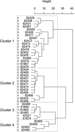
Figure 4. Box plots of cluster variables (A) SJI duration, (B) SJI visits, (C) JDF duration, (D) JDF visits, (E) ADM duration, (F) ADM visits, (G) CPS duration, and (H) CPS visits by cluster group. The P-values are from Kruskal–Wallis tests for differences between clusters. Letters indicate significant differences between clusters from post hoc multiple comparison tests. Boxes with the same letter are not significantly different (i.e., a box labeled “a” is not significantly different than another labeled “a”). Boxes with different letters are significantly different (i.e., “a” is significantly different than “b”). Boxes with both letters are not significantly different from either (i.e., “ab” is not significantly different from “a” or “b”).

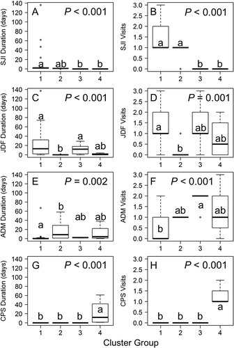
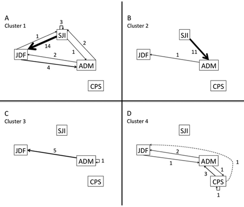
Cluster 1 had a Jaccard bootstrap mean value of 0.68 and included 18 fish, all of which were tagged in the SJI, whose detections centered in that area and JDF (Table 1). None of these fish was detected in CPS. Four of these fish spent 24–136 d in the SJI, and 14 spent 1–3 d there; six visited the SJI two to three times, and 12 visited only once (Figure 4A, B). Nine of these fish spent 16–137 d in JDF, and the other nine spent 0–10 d; 15 visited JDF one to three times, and the other three were never detected there (Figure 4C, D). One fish spent 67 d at ADM, and the other 17 spent 0–4 d there; five fish visited one to two times, and 13 were never detected at ADM (Figure 4E, F)

Table 1. Basin fidelity and interbasin movement data. The data for the eight variables (total duration in and number of visits to each basin) are provided for all 40 Chinook Salmon included in the cluster analysis.

			Total duration (d)				Number of visits
Cluster	Serial number	Tagging location	SJI	JDF	ADM	CPS	SJI	JDF	ADM	CPS
1	61867	SJI	1	10	0	0	1	1	0	0
1	82426	SJI	2	2	3	0	2	2	2	0
1	82427	SJI	2	137	0	0	2	1	0	0
1	82429	SJI	136	0	0	0	1	0	0	0
1	82431	SJI	62	0	0	0	2	0	0	0
1	82450	SJI	3	10	0	0	3	3	0	0
1	82452	SJI	1	17	0	0	1	2	0	0
1	82455	SJI	1	22	0	0	1	2	0	0
1	82458	SJI	24	0	0	0	1	0	0	0
1	82460	SJI	1	74	0	0	1	1	0	0
1	82467	SJI	47	32	0	0	2	1	0	0
1	82472	SJI	1	58	4	0	1	3	1	0
1	82473	SJI	1	49	1	0	1	1	1	0
1	82474	SJI	3	1	2	0	1	1	1	0
1	82476	SJI	2	16	0	0	1	1	0	0
1	82477	SJI	3	9	67	0	2	2	1	0
1	82478	SJI	1	3	0	0	1	2	0	0
1	82479	SJI	1	26	0	0	1	1	0	0
2	82424	SJI	1	0	9	0	1	0	1	0
2	82425	SJI	1	0	57	0	1	0	1	0
2	82432	SJI	1	0	2	0	1	0	1	0
2	82433	SJI	1	0	1	0	1	0	1	0
2	82454	SJI	1	0	18	0	1	0	1	0
2	82456	SJI	1	0	1	0	1	0	1	0
2	82457	SJI	1	0	8	0	1	0	1	0
2	82468	SJI	1	0	58	0	1	0	1	0
2	82469	SJI	1	0	23	0	1	0	1	0
2	82470	SJI	1	0	1	0	1	0	1	0
2	82471	SJI	1	0	1	0	1	0	1	0
2	82486	ADM	0	1	35	0	0	1	1	0
3	40321	ADM	0	18	1	0	0	3	1	0
3	61864	ADM	0	2	3	0	0	1	2	0
3	61869	ADM	0	11	3	0	0	1	2	0
3	61874	ADM	0	29	2	0	0	2	2	0
3	82485	ADM	0	13	2	0	0	1	2	0
3	82488	ADM	0	0	2	0	0	0	2	0
4	82462	CPS	0	0	0	61	0	0	0	1
4	82463	CPS	0	1	2	2	0	1	1	1
4	82465	CPS	0	4	38	22	0	2	3	2
4	82466	CPS	0	0	6	1	0	0	1	1

Cluster 2 had a Jaccard bootstrap mean value of 0.75 and included 12 fish with very few detections (Table 1). Eleven fish tagged within the SJI had a single 1-d visit there and were not detected in JDF or CPS (Figure 4). There was also one fish tagged in ADM that was never detected in the SJI or CPS and had a single 1-d visit to JDF (Figure 4). All 12 fish in this cluster visited ADM once; five spent 1–2 d, and seven spent 8–58 d there (Figure 4E, F).

Cluster 3 had a Jaccard bootstrap mean value of 0.78 and included six fish, all tagged within ADM (Table 1). None of the fish was detected in the SJI (Figure 4A, B); five spent 2–29 d in the JDF on one to three visits, and the other was never detected there (Figure 4C, D). All six fish spent 1–3 d in ADM on one to two visits (Figure 4E, F). None of the fish in this cluster was detected in CPS (Figure 4G, H).

Cluster 4 had a Jaccard bootstrap mean value of 0.78 and included four fish, all tagged within CPS (Table 1). None was detected in the SJI (Figure 4A, B). Two of them spent 1–4 d in the JDF on one to two visits, whereas the other two were never detected there (Figure 4C, D). Three of the fish spent 2–38 d in ADM on one to three visits, and the other was not detected there. In CPS, two spent 1–2 d on a single visit, and the other two spent 22–61 d on one or two visits (Figure 4G, H).

Individual fish traveled to the four receiver regions in various ways (Figure 5). Fish from clusters 1 and 2, all tagged in the SJI with the exception of one from ADM, exhibited similarly wide distributions including the SJI, JDF, and ADM, with the primary difference being that cluster 1 fish spent more time in the SJI and JDF, whereas cluster 2 fish spent more time in ADM (Figures 4, 5). Cluster 3 fish predominantly traveled to JDF from ADM yet spent little time in ADM, even though they were tagged in that area and visited it numerous times (Figures 4, 5). Cluster 4 fish spent most of their time in CPS and ADM, with, at most, short visits to JDF (Figures 4, 5). At least one fish from each of the four clusters was detected in the JDF and ADM (Figures 4, 5). In contrast, only fish from clusters 1 and 2 were detected in the SJI, while only fish from cluster 4 were detected in CPS (Figures 4, 5).

Figure 5. Regional movement patterns by cluster group. Directional arrows are weighted by the number of movements (shown adjacent). Straight lines represent fish undergoing interregional movements, whereas U-shaped lines represent fish that were detected exclusively in their tagging region. In (D), the dashed line represents a fish that was detected in the CPS and then the JDF without being detected in the ADM, which means that it either departed the CPS via the Whidbey basin or via the ADM, where it avoided detection by the ADM array.

The groups of receivers in CPS and the SJI were too heterogeneous in locations to provide detailed information about local scales of movement, but the two lines of receivers at JDF and ADM were examined for patterns of distribution in terms of distance from shore, depth of water, and numbers of times the fish crossed the U.S.–Canadian border (at JDF). At both arrays, Chinook Salmon detections primarily occurred at receivers in deeper water (Figure 2). The main exception to this pattern was the high proportion of detections at the receivers nearest the Canadian shoreline of the JDF array (Figure 2).

At the JDF array, 24 different fish were detected. Individuals crossed the international boundary 0–124 times (calculated as the number of times a fish was sequentially detected at a receiver on the American and then Canadian side of the array, and vice versa). Twenty fish crossed the boundary 1–10 times, and three fish crossed more than 10 times. Only one fish was exclusively detected in American waters of the JDF array, and the other 23 were detected in Canadian waters at least once.

Discussion

We detected four Chinook Salmon distribution patterns that were associated with the basins where they had been caught and tagged, even though the tagging areas are relatively proximate (Figure 1). Specifically, none of the salmon tagged in the CPS was detected in the SJI and vice versa (Figures 4, 5), though the areas are only ca. 85 km apart. On the other hand, one Chinook Salmon tagged in the SJI was recorded ca. 70 km away at ADM a day later, exhibiting how quickly salmon can travel. One might propose that so few salmon entered CPS because it is simply not suitable habitat, but a large fraction of the resident Chinook Salmon produced in hatcheries in CPS were recovered in fisheries there (Chamberlin and Quinn 2014). Additionally, an acoustic study of resident Chinook Salmon depth distribution recorded nearly 15,000 detections of 24 individual fish in CPS and the adjacent waters (Smith et al. 2015). Consequently, the limited exchange among regions cannot be explained by barriers to movement or habitat unsuitability. Admiralty Inlet may be a transition zone between basins as well as a rearing area (Chamberlin and Quinn 2014), as indicated by the movement of fish from all tagging areas through this region (Figures 4, 5). Hence, there may be more exchange between the CPS and ADM, and between the ADM and SJI, than between the SJI and CPS.

Resident Chinook Salmon tagged in the CPS occupied that area and ADM but not the SJI, whereas salmon tagged in the SJI spent time in the JDF and ADM as well as the SJI (Figures 4, 5). These data suggested that CPS residents may occupy a more limited area or less often move north and west, whereas salmon tagged in the SJI occupy a wider area. Additionally, fish tagged in the SJI exhibited more variability in residency and movement patterns (Figures 3, 5). The complexity of spatial distribution exhibited by resident Chinook Salmon tagged in the SJI highlights their differences in basin fidelity, degree of residency, and movement patterns from their counterparts in Puget Sound.

The exact cause of the dramatically higher proportions of fish tagged in the CPS and ADM that were never detected is unknown. There were no handling differences during the tagging process between these two groups of Chinook Salmon and those tagged in the SJI that would result in the disparate detection proportions. The recreational harvest of study fish was also unlikely to be the cause of the difference because none of the salmon tagged in the CPS and only 2 of 23 from the ADM were above the Washington legal minimum size of 22 in (~559 mm) in WDFW MA 5–13 (WDFW 2016). Additionally, none of the CPS tagged fish and only 5 of 23 ADM tagged fish were above the Canadian legal minimum size of 450 mm in DFO MA 19–21 (DFO 2016). Lastly, no fish tagged in the CPS or ADM were above the legal minimum size of 620 mm in DFO MA 18 and a specific portion of MA 19 (DFO 2016).

Potential causes of the difference in the proportion of detected fish between basins included the distribution of receivers and differential mortality. Unlike the ADM or JDF, the CPS contained isolated receivers instead of an array that could have provided more complete coverage of Chinook Salmon movements at the northern end of the area (Figure 1). While there was an array within the ADM, there were no receivers at the junction between the ADM and the adjacent Whidbey basin (Figure 1). Therefore, fish tagged in the ADM and those tagged in the CPS that moved into the ADM may have entered the Whidbey basin without being detected. Moreover, fish tagged in the CPS that moved south in Puget Sound would have encountered an even lower density of receivers than those staying in the CPS or moving north. Differences in detection probability are the most plausible reason for the spatial patterns of detections, but we have no way to distinguish lack of detection from mortality. While the resulting low sample sizes of fish tagged in the CPS (four) and ADM (seven) that were later detected necessitate careful interpretation, as these few individuals may not fully represent the behavior of their populations, the findings nevertheless provide valuable information on movement patterns.

The different distributions of the CPS and SJI resident Chinook Salmon may affect their likelihood of interception in different fisheries. The CPS residents appear most likely to get captured in Canadian waters of the JDF, when outside of their primary range. However, due to their fidelity for the CPS, Chinook Salmon from this region seem to have a lower chance of being intercepted in these more distant marine areas than conspecifics from more northerly origins. In contrast, residents feeding in the SJI seem likely to be caught in the JDF, Haro Strait, and the southern Strait of Georgia.

In addition to the implications of salmon movement patterns for the management of fisheries, the localized distributions of resident Chinook Salmon may affect their exposure to chemical contaminants. Compared with the Strait of Georgia, Puget Sound has almost 10 times more people relative to its drainage area, one-third the surface area, one-sixth the volume, and half the summer water turnover rate, all of which may increase contaminant retention and loading (West et al. 2008). Puget Sound resident Chinook Salmon had the highest concentrations of contaminants of all populations and salmon species sampled on the West Coast, as they occupy a heavily urbanized basin containing forage fish that feed in a contaminated food web (S. M. O’Neill and coworkers, paper presented at the 2006 Southern Resident Killer Whale Symposium; extended abstract available at http://wdfw.wa.gov/publications/01034/). O’Neill and West (2009) attributed the wide range of polychlorinated biphenyl (PCB) levels in resident Chinook Salmon to variation in the degree of residency and distribution, but they noted that the movements of the fish they sampled were unknown.

The CPS resident Chinook Salmon tended to remain within the more polluted waters of ADM and CPS, whereas SJI resident Chinook Salmon tended to occupy the less contaminated SJI and JDF (Mearns 2002; Chamberlin and Quinn 2014; this study: Figures 4, 5). Consequently, the different distributions of CPS versus SJI residents may result in dissimilar contaminant loads, which could explain the variability of PCB levels in resident Chinook Salmon sampled by O’Neill and West (2009). The potential disparity in contaminant concentration between these two groups of subadult resident Chinook Salmon would parallel regional contaminant differences documented in populations of blue mussel Mytilus edulis (Mearns 2002), Pacific Herring Clupea pallasii (West et al. 2008), and harbor seals Phoca vitulina (Ross et al. 2004; Cullon et al. 2005) that inhabit southern and central Puget Sound versus the SJI and the southern Strait of Georgia.

Subadult Chinook Salmon are mobile, pelagic mesopredators, physically capable of moving long distances in the open ocean and along the continental shelf (Weitkamp 2009; Sharma and Quinn 2012), but some seem to remain within tens of kilometers of their natal river for much of their marine residence period. The diversity in salmon migration patterns exemplifies many basic themes in migratory behavior, including partial migration (Chapman et al. 2011a; Rohde et al. 2013) and individual variation (Chapman et al. 2011b). In the case of resident behavior by anadromous salmon, the pattern seems to be influenced by a combination of genetics (Quinn et al. 2011), rearing history (Chamberlin et al. 2011a), and environmental factors (Rohde et al. 2014), making it an intriguing alternative to the long migrations for which they are famous. Resident Chinook Salmon in CPS and the SJI exhibit different distributions and substantial variability in their extent of movement and degree of basin fidelity and jointly represent a less migratory but ecologically important part of the gradient of life histories (Quinn and Myers 2004) expressed by anadromous salmonids. This diversity of migratory patterns presents challenges for fishery regulations, but the protection of life history complexity is an important part of efforts to conserve and restore the Pacific Northwest’s iconic Chinook Salmon.

Acknowledgments

We thank the crews of the sportfishing charter vessels and especially Jay Field for capturing the fish for tagging, Jennifer Scheuerell for data management, Fred Goetz for his role in the formation of this project, Sandra O’Neill for input that helped shape the work and interpret the results, and Kinsey Frick, Todd Sandell, Jason Hall, Joshua Chamberlin, and many others for field assistance. We thank Scott Veirs, Tina Echeverria, and Beam Reach for their assistance with deploying and retrieving receivers, and the many agencies that deployed and retrieved receivers and shared data with us, especially the Pacific Ocean Shelf Tracking Project. We are also very grateful to the many landowners who gave us permission to deploy receivers from their docks or near their property. Funding for this project was provided by the State of Washington’s Salmon Recovery Funding Board through the Recreation and Conservation Office; National Oceanic and Atmospheric Administration (NOAA) Fisheries; the Clarence H. Campbell Endowed Lauren Donaldson Scholarship in Ocean and Fishery Sciences; the H. Mason Keeler Endowment and Richard and Lois Worthington Endowment at the School of Aquatic and Fishery Sciences, University of Washington; and the Achievement Rewards for College Scientists Foundation, Seattle Chapter, via the Barton family. Permits for the deployment of receivers were obtained from NOAA Fisheries, the Washington Department of Natural Resources, WDFW, and San Juan County. Permits for the capture and handling of fish were obtained from NOAA Fisheries, WDFW, and the University of Washington’s Institutional Animal Care and Use Committee.

References

- Baker, R. R. 1978. The evolutionary ecology of animal migration. Holmes and Meier, New York.
- Bauer, S., and B. J. Hoye. 2014. Migratory animals couple biodiversity and ecosystem functioning worldwide. Science 344:1242552.
- Chamberlin, J. W., T. E. Essington, J. W. Ferguson, and T. P. Quinn. 2011a. The influence of hatchery rearing practices on salmon migratory behavior: is the tendency of Chinook Salmon to remain within Puget Sound affected by size and date of release? Transactions of the American Fisheries Society 140:1398−1408.
- Chamberlin, J. W., A. N. Kagley, K. L. Fresh, and T. P. Quinn. 2011b. Movements of yearling Chinook Salmon during the first summer in marine waters of Hood Canal, Washington. Transactions of the American Fisheries Society 140:429–439.
- Chamberlin, J. W., and T. P. Quinn. 2014. Effects of natal origin on localized distributions of Chinook Salmon, Oncorhynchus tshawytscha, in the marine waters of Puget Sound, Washington. Fisheries Research 153:113–122.
- Chapman, B. B., C. Brönmark, J.-A. Nilsson, and L.-A. Hansson. 2011a. The ecology and evolution of partial migration. Oikos 120:1764–1775.
- Chapman, B. B., K. Hulthén, D. R. Blomqvist, L.-A. Hansson, J.-A. Nilsson, J. Brodersen, P. A. Nilsson, C. Skov, and C. Brönmark. 2011b. To boldly go: individual differences in boldness influence migratory tendency. Ecology Letters 14:871–876.
- Cullon, D. L., S. J. Jeffries, and P. S. Ross. 2005. Persistent organic pollutants in the diet of harbor seals (Phoca vitulina) inhabiting Puget Sound, Washington (USA), and the Strait of Georgia, British Columbia (Canada): a food basket approach. Environmental Toxicology and Chemistry 24:2562–2572.
- Cullon, D. L., M. B. Yunker, C. Alleyne, N. J. Dangerfield, S. O’Neill, M. J. Whiticar, and P. S. Ross. 2009. Persistent organic pollutants in Chinook Salmon (Oncorhynchus tshawytscha): implications for resident killer whales of British Columbia and adjacent waters. Environmental Toxicology and Chemistry 28:148–161.
- DFO (Department of Fisheries and Oceans Canada). 2016. BC sport fishing guide. Available: http://www.pac.dfo-mpo.gc.ca/fm-gp/rec/index-eng.html. (January 2017).
- Dingle, H. 1996. Migration: the biology of life on the move. Oxford University Press, New York.
- Giraudoux, P. 2015. pgirmess: data analysis in ecology. R package version 1.6.3. Available: http://CRAN.R-project.org/package=pgirmess. ( December 2016).
- Good, T. P., S. F. Pearson, P. Hodum, D. Boyd, B. F. Anulacion, and G. M. Ylitalo. 2014. Persistent organic pollutants in forage fish prey of rhinoceros auklets breeding in Puget Sound and the northern California Current. Marine Pollution Bulletin 86:367–378.
- Gotelli, N. J., and A. M. Ellison. 2004. A primer of ecological statistics. Sinauer, Sunderland, Massachusetts.
- Hall, J. E., J. Chamberlin, A. N. Kagley, C. Greene, and K. L. Fresh. 2009. Effects of gastric and surgical insertions of dummy ultrasonic transmitters on juvenile Chinook Salmon in seawater. Transactions of the American Fisheries Society 138:52−57.
- Haw, F., H. O. Wendler, and G. Deschamps. 1967. Development of Washington State salmon sport fishery through 1964. Washington Department of Fisheries Research Bulletin 7.
- Healey, M. C., and C. Groot. 1987. Marine migration and orientation of ocean-type Chinook and Sockeye Salmon. Pages 298–312 in M. J. Dadswell, R. J. Klauda, C. M. Moffitt, R. L. Saunders, R. A. Rulifson, and J. E. Cooper, editors. Common strategies of anadromous and catadromous fishes. American Fisheries Society, Symposium 1, Bethesda, Maryland.
- Hennig, C. 2014. Fpc: flexible procedures for clustering. R package version 2.1-9. Available: https://cran.r-project.org/web/packages/fpa/fpc.pdf. (January 2017).
- Jonsson, B., and N. Jonsson. 2011. Ecology of Atlantic Salmon and Brown Trout: habitat as a template for life histories. Springer, New York.
- Mearns, A. J. 2002. Long-term contaminant trends and patterns in Puget Sound, the Strait of Juan de Fuca, and the Pacific coast. In T. Droscher, editor. Proceedings of the 2001 Puget Sound Research Conference. Puget Sound Water Quality Action Team, Olympia, Washington.
- Melnychuk, M. C., V. Christensen, and C. J. Walters. 2013. Meso-scale movement and mortality patterns of juvenile Coho Salmon and steelhead trout migrating through a coastal fjord. Environmental Biology of Fishes 96:325–339.
- Moore, M. E., B. A. Berejikian, F. A. Goetz, A. G. Berger, S. S. Hodgson, E. J. Connor, and T. P. Quinn. 2015. Multi-population analysis of Puget Sound steelhead survival and migration behavior. Marine Ecology Progress Series 537:217–232.
- Morales, J. M., P. R. Moorcroft, J. Matthiopoulos, J. L. Frair, J. G. Kie, R. A. Powell, E. H. Merrill, and D. T. Haydon. 2010. Building the bridge between animal movement and population dynamics. Philosophical Transactions of the Royal Society B 365:2289–2301.
- O’Neill, S. M., and J. E. West. 2009. Marine distribution, life history traits, and the accumulation of polychlorinated biphenyls in Chinook Salmon from Puget Sound, Washington. Transactions of the American Fisheries Society 138:616–632.
- O’Neill, S. M., J. E. West, and J. C. Hoeman. 1998. Spatial trends in the concentration of polychlorinated biphenyls (PCBs) in Chinook (Oncorhynchus tshawytscha) and Coho salmon (O. kisutch) in Puget Sound and factors affecting PCB accumulation: results from the Puget Sound Ambient Monitoring Program. Pages 312–328 in Puget Sound research ’98 proceedings. Puget Sound Water Quality Action Team, Olympia, Washington.
- Pressey, R. T. 1953. The sport fishery for salmon on Puget Sound. Washington Department of Fisheries Fisheries Research Papers 1:33–48.
- Quinn, T. P. 2005. The behavior and ecology of Pacific salmon and trout. University of Washington Press, Seattle.
- Quinn, T. P., J. Chamberlin, and E. L. Brannon. 2011. Experimental evidence of population-specific spatial distributions of Chinook Salmon, Oncorhynchus tshawytscha. Environmental Biology of Fishes 92:313–322.
- Quinn, T. P., and K. W. Myers. 2004. Anadromy and the marine migrations of Pacific salmon and trout: Rounsefell revisited. Reviews in Fish Biology and Fisheries 14:421–442.
- R Core Team. 2015. R: a language and environment for statistical computing. R Foundation for Statistical Computing, Vienna.
- Rohde, J., K. L. Fresh, and T. P. Quinn. 2014. Factors affecting partial migration in Puget Sound Coho Salmon (Oncorhynchus kisutch). North American Journal of Fisheries Management 34:559–570.
- Rohde, J., A. N. Kagley, K. L. Fresh, F. A. Goetz, and T. P. Quinn. 2013. Partial migration and diel movement patterns in Puget Sound Coho salmon. Transactions of the American Fisheries Society 142:1615–1628.
- Ross, P. S., S. J. Jeffries, M. B. Yunker, R. F. Addison, M. G. Ikonomou, and J. C. Calambokidis. 2004. Harbor seals (Phoca vitulina) in British Columbia, Canada, and Washington State, USA, reveal a combination of local and global polychlorinated biphenyl, dioxin, and furan signals. Environmental Toxicology and Chemistry 23:157–165.
- Ryan, W. B. F., S. M. Carbotte, J. Coplan, S. O’Hara, A. Melkonian, R. Arko, R. A. Weissel, V. Ferrini, A. Goodwillie, F. Nitsche, J. Bonczkowski, and R. Zemsky. 2009. Global Multi-Resolution Topography (GMRT) synthesis data set. Geochemistry, Geophysics, Geosystems [online serial] 10:Q03014.
- Sharma, R., and T. P. Quinn. 2012. Linkages between life history type and migration pathways in freshwater and marine environments for Chinook Salmon, Oncorhynchus tshawytscha. Acta Oecologica 41:1–13.
- Smith, J. M., K. L. Fresh, A. N. Kagley, and T. P. Quinn. 2015. Ultrasonic telemetry reveals seasonal variation in depth distribution and diel vertical migrations of sub-adult Chinook and Coho Salmon in Puget Sound. Marine Ecology Progress Series 532:227–242.
- Trudel, M., J. Fisher, J. A. Orsi, J. F. T. Morris, M. E. Thiess, R. M. Sweeting, S. Hinton, E. A. Fergusson, and D. W. Welch. 2009. Distribution and migration of juvenile Chinook Salmon derived from coded wire tag recoveries along the continental shelf of western North America. Transactions of the American Fisheries Society 138:1369−1391.
- Waples, R. S., D. J. Teel, J. M. Myers, and A. R. Marshall. 2004. Life-history divergence in Chinook Salmon: historic contingency and parallel evolution. Evolution 58:386–403.
- Washington State Department of Health. 2006. Human health evaluation of contaminants in Puget Sound fish. Washington State Department of Health, Division of Environmental Health, Publication 334–104, Olympia.
- WDFW (Washington Department of Fish and Wildlife). 2016. Fishing and shellfishing regulations & seasons. Available: http://wdfw.wa.gov/fishing/regulations. (January 2017).
- Weitkamp, L. A. 2009. Marine distributions of Chinook Salmon from the West Coast of North America determined by coded wire tag recoveries. Transactions of the American Fisheries Society 139:147–170.
- West, J. E., S. M. O’Neill, and G. M. Ylitalo 2008. Spatial extent, magnitude, and patterns of persistent organochlorine pollutants in Pacific Herring (Clupea pallasi) populations in the Puget Sound (USA) and Strait of Georgia (Canada). Science of the Total Environment 394:369–378.