Rent growth near rail stations after the Great Recession

Abstract

This study provides an incisive analysis of U.S. rail station area rent trends from 2012 to 2016, post-Great Recession. Utilizing Ordinary Least Squares (OLS), Hierarchical Spatial Autoregressive (HSAR), and Geographically Weighted Regression (GWR) models, it uncovers complex interplays between rent changes and socioeconomic, as well as built environment factors. Key findings reveal that increased rents are associated with walkability, higher housing density, and predominantly White neighborhoods. Conversely, rent decreases correlate with diverse land use, higher Black population percentages, and locations further from rail stations or business districts. These results are critical for understanding rent dynamics in transit-oriented development areas, impacting diverse housing market sectors, including workforce and affordable housing. The study’s regional analysis highlights the need for geographically tailored approaches. This research informs policy on housing development and affordability, aiming to mitigate displacement risks for low-income, transit-dependent communities in gentrifying urban areas.

Keywords:

• Rail stations
• Great Recession
• transit
• rent
• transit oriented development
• transit oriented communities

Introduction

A growing body of research examines the influence of improved transit accessibility, the built environment and transit-oriented development (TOD), and associated amenities on land values (Knaap et al., 2001; McIntosh et al., 2013; Xu, 2015; Yan et al., 2012). Often, the existing literature confirms that investments in transit and built environments with higher levels of walkability and density, also characterized as TODs and transit-oriented communities (TOCs), increase home values if they improve access significantly (Appleyard et al., 2019; Benjamin & Sirmans, 1994; Zuk et al., 2015). While the definitions overlap, generally TOCs encompass all property in a station area whereas TODs can refer to a station area, a particular project, or a general concept (Renne & Appleyard, 2019). Also, TOC is becoming associated with equity initiatives stemming from high costs and gentrification associated with TOD (Song, 2023). Nevertheless, the definitions can be confusing and while many studies focus on land values or home values, research into the influence of transit and built environment variables on rent growth is limited, and can therefore inform the literature on TOD, real estate and urban planning.

A study conducted on rental housing in U.S. cities found that approximately 70% of renter households had incomes below the national median. More than 40% had income in the bottom quartile (Fernald, 2011). This study also observed that renters are more ethnically and racially diverse than homeowners, and minority households, including foreign-born residents, account for a large part of the rental market. These findings are consistent with Glaeser et al. (2008), who found that rental housing is associated with a higher percentage of foreign-born residents leasing apartments close to public transportation networks. According to Apell (2014), minorities account for a larger proportion of renters than Whites because of their lower-income status. Apell further pointed out that low car ownership compelled minorities to live in transit zones to access public transportation (Apell, 2014).

From an equity perspective, it is concerning to see rental values increase around a station, leading to the pricing out of lower-income, transit-dependent households. Higher rents may cause displacement from transit-rich neighborhoods, causing low-income residents to find housing in cheaper areas with little or no public transportation coverage (Appleyard et al., 2019; Belzer et al., 2006). Hence, to ensure equitable TOCs and serve transit-dependent populations, there is a need to understand the rental dynamics in station areas. This includes the concept of location affordability, which several studies have examined with somewhat conflicting results (Renne et al., 2016; Singer, 2021; Smart & Klein, 2017).

Identifying positive or negative influences of transit and built environment characteristics on rent will provide policymakers with the necessary information to support decisions about developing new or expand affordable housing around station areas. Such policies can help address equity concerns about transit gentrification (Zuk et al., 2015).

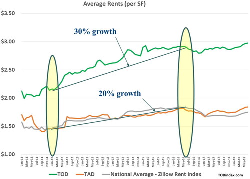
During the recovery following the Great Recession, trends in rental prices, from January 2012 to June 2016, indicate that apartments in stations identified as TODs significantly outperformed the national average and non-TOD station areas (known as transit-adjacent developments (TADs). TODs were characterized as station areas with high levels of walkability and density, and accounted for about one-third of all stations. Figure 1 shows that prices in TODs appreciated by 30% compared to a growth of 20% in TADs, which was the same as the national average.

Figure 1. Rents in TOD and TADs compared to the National Average, 2012–2016. Source: TOD Index.

This study analyzes rent trends in all station areas in the post-recession era and allows for built environment variables, including density, walkability, land use mix, distance to transit, and other variables to isolate significant predictors of rent change. This approach then allows for a more detailed understanding of what factors are associated with rent growth or decline in TODs and TOCs. This study utilizes a hierarchical spatial autoregressive model (HSAR) and geographically weighted regression (GWR) in comparison to a base ordinary least squares (OLS) regression model. The results show that OLS and HSAR models follow the same pattern, revealing that density, walkability, percentage White, and income are positively associated with increases in rents. In contrast, land use mix, percentage Black, increasing distance to the station, and distance to the central business district (CBD) were each associated with downward pressure on rents. The GWR model revealed the significance and influence of independent variables vary from region to region and within a given region.

Literature

This section discusses the limited available research on rental values in transit station areas. Benjamin and Sirmans (1994) investigated the residential rental values of 250 apartments from eighty-one complexes located near Washington D.C. Metro rail stations. The study examined monthly rent as the dependent variable and apartment physical characteristics, area code, and distance to the Metro as independent variables. The authors found that as the distance to the Metro increased, the residential income properties rental values decreased. When the length increased to one mile from the metro station, rent declined by more than 20%.

Similarly, Feinstein and Allen (2008) used Geolytics data. They analyzed the difference in growth rates in rental values in 31 census tracts located within 1.4 miles from Boston’s expanded red line transit stations versus the rest of the census tracts in Boston. The study found that rents in those census tracts near the transit station increased 10.2% greater than the rest of the census tracts. Brown (2016) compared the change in rental values in census tracts located within 0.5-mile, 0.5 to 2-mile, 2 to 5-mile radii of transit stations versus the rest of the Los Angeles County. The study found that the change in median rents was higher (32% growth) within a 0.5-mile radius of Orange Line stations than the other areas (24% growth), confirming the association of increased rental values within proximity of transit.

Apell (2014) developed a model to predict the rental values of the properties located within a one-mile radius of station areas in six metropolitan statistical areas (MSAs), using 1990–2000 census block-level data. The study area included 100 TODs and 152 non-TODs. The author used demographic, socioeconomic, and location variables as independent variables and 2010 rental values as the dependent variable. This study revealed that rental values in TOD block groups exceeded non-TOD values by 49%, implying that TODs are less effective in keeping housing costs down compared with non-TODs.

Nelson (2016) analyzed the association of office, retail, and rental apartment rents with the presence of different types of transit in bands of 0.5 and 0.5–1 mile from transit corridors in 25 metropolitan counties using CoStar data. As the dependent variable, the author used asking rent during the first quarter of 2015 and utilized structural information and location variables (including a regional dummy variable) as independent variables. The study found that the streetcar transit had the most robust outcomes compared to the other transit modes. Light rail transit (LRT) also had significant, positive associations with rents. On the other hand, results for bus rapid transit (BRT) were mixed. BRT negatively associated retail rents within the 0.5-mile distance band but positively related to rental apartments. The association with office rents was not statistically significant. Across all development types, proximity to commuter rail transit corridors either had an insignificant or negative association with rental values.

Using the Geolytics neighborhood change database and American Community Survey (ACS) 2009–2013, Deka (2017) studied the influence of transit on rental values between 1990 and 2013 in New Jersey. This study examined the presence of a station, ethnicity, education, and income as independent variables. In contrast to the previous studies, Deka (2017) did not find any association between rental values and transit proximity.

All the studies discussed above have adopted two standard methods to study the effect of transit proximity on rent. The first is to compare the change in rental values of a census tract located close to transit stations with the more extensive MSAs control tracts (Brown, 2016; Feinstein & Allen, 2008). The second method is developing models analyzing TOD policy or distance to transit on rental values (Apell, 2014; Benjamin & Sirmans, 1994; Deka, 2017; Nelson, 2017). Apell’s 2014 study represented TOD policy with a dummy variable in determining the influence on rental values. However, his study did not control for the effect of other individual TOD variables on rent. Another limiting factor in the research is that most of the other studies focused on rent using only one year of cross-sectional data (Benjamin & Sirmans, 1994; Nelson, 2016).

With such few constrained studies, we face a limited understanding of rental values in station areas. We address this gap in the literature by examining data spanning the post-recession period from January 2012 to June 2016. We analyze the influence of individual built environment variables, including key built environment variables (density, land use mix, and walkability), socio-demographics (percent Black and White), income, and distance to the station and central business district (CBD).

Higgins and Kanaroglou (2016) propose three key recommendations for improving research on Land Value Uplift (LVU) related to accessibility and TODs. They emphasize the importance of considering the specific context of transit station areas, particularly the characteristics associated with TODs. They argue for incorporating factors like density, mixed-use development, walkability, and street network connectivity in LVU models to capture the full impact of these elements on property values. They also recommend employing advanced hedonic modeling techniques that account for spatial dependencies and heterogeneity. They highlight the significance of controlling for relevant variables, such as regional and local accessibility measures, neighborhood quality indicators, and economic growth trends. By following these recommendations, researchers can enhance the validity and empirical robustness of LVU models.

Methodology

This study developed models to predict rent changes from January 2012 to June 2016 in around 23,000 census tracts located within a five-mile radius of rail stations. All of the stations in the study were opened prior to 2010. Many studies have examined the impact of rents within a half-mile of railway stations, which is the typical distance utilized for most studies on TOD, but some studies have found that the influence of stations on price can extend beyond 2–3 miles from stations (Bowes & Ihlanfeldt, 2001; Debrezion et al., 2007; McMillen & McDonald, 2004). This study examined rents from stations to capture the widest possible impacts that could extend 5 miles from the stations. This study provides a measure of the centroid of each census tract to the station so distance is treated as an independent variable for each tract.

The dates were chosen to reflect the start of real estate market recovery to a period sufficiently into the recovery. Zillow provided a special run of the data at the census tract level. Normally Zillow reports data at the Zip code level as the smallest unit of analysis.

We adopted three types of regression techniques in R 3.5.1:

1. Ordinary Least Squares (OLS)

2. Hierarchical Spatial Autoregressive (HSAR) model

3. Geographically Weighted Regression (GWR) models

Ordinary Least Squares (OLS)

OLS regression is a statistical approach to determine the relationship between one or more independent variables and a dependent variable. It establishes the relationship between the independent and dependent variables by minimizing the sum of the squares in the difference between the observed and predicted values of the dependent variable. This study uses the OLS model as the base model to allow for comparison with the HSAR and GWR models. The equation of OLS is:

$$y=\alpha +{\beta }_i{x}_i+\epsilon$$

Y is the dependent variable; α is the intercept; x_i is the Ith independent variable; β_i is the coefficient of ith independent variable; ε is the random error.

Hierarchical Spatial Autoregressive (HSAR) model

We developed an HSAR model for spatial data with a hierarchical structure. This model brings together the multilevel models and spatial econometrics. It is suitable for a simultaneous capturing of the potential spatial dependence (autocorrelations) at each level of the data hierarchy arising from the geographical proximity effect and the contextual effect from higher-level units (region) upon lower-level units (census tracts) (Dong & Harris, 2015).

The formulation of a HSAR model is as follows: $$y_{i,j}=\rho *W_i*y+{x’}_{I,j}*\beta +{z’}_j*\gamma +{\theta }_j+{\epsilon }_{i,j}$$ $${\theta }_j=\lambda *M_j*\theta +{\mu }_j$$ $${\epsilon }_{i,j}\sim N(0,{{\sigma }^2}_e)$$ $${\mu }_j\sim N(0,{{\sigma }^2}_u)$$ where i = 1,2,…,n_j and j = 1,2,…,J are indicators of lower and higher-level spatial units. n_j is the number of lower-level units in the jth higher-level unit and ${\sum }_{j=1}^j=N*x_{i,j }^{\prime }$ and $z_{j }^{\prime }$ represent vectors of lower-and higher-level independent variables. β and γ are regression coefficients to estimate. θ, an N × J vector of higher-level random effects, also follows a simultaneous autoregressive process. W and M are two spatial weights matrices (or neighborhood connection matrices) at the lower and higher levels, defining how spatial units at each level are connected. ρ and λ are spatial autoregressive parameters measuring the strength of the dependencies/correlations at the two spatial scales.

The HSAR model becomes a standard multilevel model when ρ and λ are both equal to zero and a standard spatial econometric model when λ and σ²_u are both equal to zero.

Geographically Weighted Regression (GWR) model

The GWR model explores the spatially varying relationships between the dependent and independent variables. According to Guo, Ma, and Zhang, the estimation procedure of GWR is as follows: (i) draw a circle of a given bandwidth, h, around one particular location i (the center), (ii) calculate a weight for each neighboring observation according to the distance between the neighbor and the center by applying selected distance-decay Kernel function, and (iii) estimate the model coefficients using weighted least-squares regression (Guo et al., 2008). The basic form of the GW regression model is: $$y_i={\mathrm{\beta }}_{i0}+\sum _{k=1}^m{\mathrm{\beta }}_{\mathit{\text{ik}}}{x}_{\mathit{\text{ik}}}+{\mathrm{\epsilon }}_i$$ where y_i is the dependent variable at location i; x_ik is the value of the kth independent variable at location i; m is the number of independent variables; β_i0 is the intercept parameter at location i; β_ik is the local regression coefficient for the kth independent variable at location i; and ε_i is the random error at location i (Lu et al., 2014).

A key aspect of GWR modeling is the weighting matrix. It sets the spatial dependency in the data. It is a function of the distance between the center and all neighbors, Kernel function, and bandwidth. There are six types of kernel functions: Global Model, Gaussian, Exponential, Box-car, Bi-square, and Tri-cube (Binbin et al., 2017). In the current study, we adopted the Bi square kernel function as shown below: $$w_{\mathit{\text{ij}}}={\left(1-{\left(d_{\mathit{\text{ij}}}/b\right)}^2\right)}^2,\mathit{\text{if }}{d}_{\mathit{\text{ij}}}\le r \mathit{\text{else}} w_{\mathit{\text{ij}}}=0$$ where w_ij is the jth element of the diagonal of the matrix of geographical weights W(u_i,v_i), and d_ij is the distance between observations i and j, and b is the bandwidth (b is the distance in case of fixed bandwidth and for the case of adaptive bandwidth, it is the distance between the point i and its Nth nearest neighbor, where N is the number of neighbors to considered to develop the weighting matrix). An optimum kernel bandwidth (either in terms of distance or the number of neighbors) for GWR is derived by minimizing the Akaike Information Criterion (AIC), which accounts for model prediction accuracy and complexity. Small bandwidths create rapid spatial variation in the results, while large bandwidths result in increasingly close to the global model solution. In the current study, we adopted the adaptive bandwidth.

Study area

This study considered 23,391 census tracts located within a five-mile radius of 4,400 transit stations in 39 regions. We removed approximately 21.9% of the census tracts due to data availability resulting in 18,278 tracts for analysis. All of these data were utilized across all three models reported below. We originally included Detroit, Harrisburg, and Jacksonville but these regions were not included in the final analysis due to missing data, resulting in 36 regions.

We divided tracts into training and testing data sets, randomly choosing 70% of the tracts (12,794) for modeling and the remaining 30% (5,484) for testing the models. We applied the same training and testing data sets for all three models. Appendix A lists all the region-specific tracts adopted in the study.

Data

The study adopted various demographic, socioeconomic, and transportation characteristics, and we removed correlated variables. We conducted trial and error methods to identify the significant independent variables for the best fitting model. Table 1 reports the final list of independent variables. The Walk Score and distance to the CBD variables are at the transit station area level (the value is the same for all the tracts), and all the remaining data is for each census tract. We obtained the information on rent prices directly from Zillow. Other data sources included the Geolytics Neighborhood Change Database, the Environmental Protection Agency’s (EPA) Smart Location Database (SLD) (based on 2010 Census data), and the National TOD Database (also based on the 2010 Census). Note that this study may be one of the first to deploy two measures of walkability. First, the Walk Score taken at the station was utilized as a measure of the walkability at the station itself. Second, the network density in terms of facility miles of pedestrian-oriented links per square mile was utilized for each tract. This allows for separate measures given that census tracts are up to five miles away from stations.

Table 1. List of variables.

RentChange (dependent variable)	Percentage of rent change in a census tract from Jan 2012 to July 2016 reported from Zillow
Density^a	Gross housing density (HU/acre) on unprotected land of a census tract
LandUse	Jobs_Pop: Standard calculation based on population and total employment: Deviation of CBG ratio of jobs/pop from the regional average ratio of jobs/pop of a census tract
Design^a	Walkability of the Census tract: Network density in terms of facility miles of pedestrian-oriented links per square mile
Income^b	Mean income per household of a census tract in 2010
PerBlack^b	Percentage of the Black population in a census tract
PerWhite^b	Percentage of the White population in a census tract
CBD^c	Distance from the transit station to CBD (Euclidean distance)
WalkScore	Walk Score at the transit station
Miles^c	Distance from census tract to the transit station (Euclidean distance)
Region_dummy^d	Region coding (dummy variable)

^aData source: Authors compilation from SLD data. Data collected for this study is based on 2010 census data. ^bData source: Geolytics neighborhood change database. ^cData source: Author’s compilation. ^dData source: National TOD database.

We extracted demographic and economic characteristics from Geolytics (2019) and built environment variables, such as population density, land use mix, and walkability from the SLD database (Ramsey & Bell 2014). The SLD provides data for every census block group in the United States; therefore, we aggregated up to the tract-level. In some cases, we averaged variables for rates (people per mile) or summed if whole numbers (i.e., number of people). We extracted the transit and the station area characteristics such as location and transit from the National TOD Database (Center for Transit-Oriented Development, 2011).

The authors used GIS software to derive the distance from the transit station to the central business district (CBD) and the distance from the tract to the nearest rail station.

In all three models, the dependent and independent variables were log-transformed to ensure more normality in the distribution.

This research utilizes a unique, multi-pronged approach, employing three regression models to explore post-recession rent trends in rail station areas across the United States. This methodology, while unconventional, contributes to the robustness and validity of our findings. By exploring the data through multiple lenses, we not only echo previous works but add depth to the narrative through the application of newer methods. This rigorous triangulation, therefore, allows for a more comprehensive understanding of the underlying rental dynamics. All of the results were calculated using the R software package.

A correlation matrix was generated, and the highest correlation was between the housing density and walkability of the census tract (Pearson Correlation = 0.7). Housing density was also negatively correlated with distance to the station (−0.6). Median income was negatively correlated with the percentage of Black residents (−0.5). Distance to the CBD and income was positively correlated (0.5). Density and income was negatively correlated (−0.4), and income and walkability of a the tract was negatively correlated (−0.4). Distance to the CBD and Walk Score of the station was slightly negatively correlated (−0.3), the Walk Score of the station and the Walkability of the census tract was sliglty negatively correlated (−0.3), distance to the station and income was slightly correlated (0.3). All other correlations was below 0.3/−0.3.

Note that an analysis was conducted on the data with and without New York, to test if the city had an impact on the results, which it did not. We therefore report the results for the entire nation, including New York.

Results

Ordinary Least Squares (OLS) model

The base model, represented by the best-fit OLS model was able to explain 57% of the variance in rent change. In this model, we choose Dallas as the reference region. The results showed that as the distance between the station and the tract increases, the percentage of change in rent decreases. Ethnicity also has a significant association with rent change. Contrary to the portion of White residents, higher shares of Black residents in a tract is associated with a decrease in rent. Like distance to the transit station, distance to CBD was negatively correlated with the rent change, indicating that as the distance to CBD increases, the percentage change in rent decreases.

Interestingly income was not statically significantly correlated with the rent change. As for the built environment variables, design and density were positively correlated with rent change, representing that as the density and pedestrian-friendly infrastructure improves in the census tracts, the percent change in rent increased. In contrast to the density and design, the land use mix was negatively correlated; the lesser the land use mix, the more the change in rents. This finding contrasts with conventional thinking on this topic, so perhaps the areas with higher jobs-population ratios were picking up places with large employment and not necessarily compatible jobs. For example, large suburban shopping malls have lots of jobs but are not necessarily compatible with TODs.

The OLS model results also show that in San Francisco, Seattle, Portland, Nashville, Denver, and Austin, the change in rents is greater than Dallas. In the rest of the regions, the change in rents is lesser than Dallas.

These results reported in Table 2 suggest the presence of heteroskedasticity in the OLS model. Both the LM statistic and the F-statistic are associated with very low p-values, indicating that the null hypothesis of homoskedasticity (constant variance of residuals) can be rejected. The Moran’s I value of approximately 0.445 indicates moderate positive spatial autocorrelation in the dataset, meaning similar values are clustered together geographically. Finally, the Koenker–Bassett test results, with a high test statistic of 656.36 and a significant p-value, strongly indicates the presence of heteroskedasticity in the OLS regression model, suggesting that the variances of the residuals are not constant and may necessitate the use of robust methods or model adjustments. These results imply that spatial relationships are important in the data and should be corrected with the HSAR and GWR models.

Table 2. OLS rent change model estimates.

Variable	Estimate	Std. error	Statistic	p-Value
(Intercept)	2.92	0.16	17.75	0.00
ln_Income	0.00	0.01	−0.30	0.76
ln_Density	0.05	0.01	6.82	0.00
ln_PerBlack	−0.06	0.00	−12.83	0.00
ln_PerWhite	0.01	0.01	2.02	0.04
ln_DisCBD	−0.08	0.01	−14.93	0.00
ln_Walkscore	0.06	0.01	5.19	0.00
ln_Miles	−0.05	0.01	−9.48	0.00
ln_Design	0.16	0.02	9.63	0.00
ln_LandUse	−0.04	0.01	−6.75	0.00
Norfolk	−2.21	0.05	−43.09	0.00
Albuquerque	−1.97	0.06	−31.01	0.00
Memphis	−1.84	0.09	−20.10	0.00
St Louis	−1.56	0.05	−34.74	0.00
Little Rock	−1.33	0.09	−14.85	0.00
Washington DC	−1.27	0.03	−42.87	0.00
Las Vegas	−1.18	0.04	−27.02	0.00
Baltimore	−1.18	0.04	−33.41	0.00
Philadelphia	−1.05	0.03	−38.49	0.00
Kansas City	−1.04	0.05	−20.12	0.00
Chicago	−0.86	0.03	−33.52	0.00
Cleveland	−0.85	0.04	−23.11	0.00
Minneapolis St Paul	−0.70	0.04	−18.69	0.00
Eugene	−0.67	0.08	−8.05	0.00
New Orleans	−0.61	0.05	−13.56	0.00
Buffalo	−0.60	0.05	−11.48	0.00
Tampa	−0.54	0.07	−8.09	0.00
Salt Lake City	−0.51	0.04	−12.96	0.00
New York	−0.43	0.03	−16.64	0.00
Atlanta	−0.42	0.04	−10.33	0.00
Sacramento	−0.37	0.04	−10.23	0.00
Pittsburgh	−0.37	0.04	−9.03	0.00
Los Angeles	−0.26	0.03	−10.28	0.00
San Diego	−0.24	0.03	−7.16	0.00
Phoenix	−0.22	0.04	−5.47	0.00
Miami	−0.21	0.03	−6.81	0.00
Boston	−0.19	0.03	−6.44	0.00
Charlotte	−0.17	0.06	−2.84	0.00
Houston	−0.06	0.05	−1.12	0.26
Austin	0.02	0.05	0.41	0.68
Seattle	0.07	0.04	1.96	0.05
Portland	0.15	0.04	3.91	0.00
Nashville	0.21	0.08	2.80	0.01
Denver	0.24	0.04	5.70	0.00
San Francisco	0.25	0.03	8.16	0.00

Residual standard error: 0.4509 on 12,749 degrees of freedom. Multiple R-squared: 0.5698, Adjusted R-squared: 0.5683. F-statistic: 383.7 on 44 and 12,749 DF, p-value: < 2.2e-16. LM Statistic: 49.56. LM-Test p-value: 1.70 × 10⁻⁹. F-Statistic: 9.98. F-Test p-value: 1.58 × 10⁻⁹. Moran’s I: 0.445. p-value: 0.001. Koenker–Bassett/Breusch–Paga Test for Heteroskedasticity. Test statistic: 656.361. p-value: 5.105079089422102e-121.

Hierarchical Spatial Autoregressive (HSAR) model

The second model to predict the percentage of rent change is developed using the HSAR technique. The model was able to explain 59% of the variance in rent change. The results are almost consistent with the OLS model.

While the OLS model serves as a foundational starting point. It provides an initial view of the relationships among variables without considering spatial or hierarchical complexities. The HSAR model goes a step further by accounting for spatial dependencies and hierarchical structures in the data. This is crucial because spatial data often exhibit autocorrelation, where observations closer in space are more correlated. Ignoring this can lead to biased estimates. While the OLS model answers the question, “What is the relationship between our predictors and the outcome, assuming independent and identically distributed residuals?” the HSAR model addresses, “How does the relationship change when we account for spatial and hierarchical structures in the data.”

One way to measure this is by using the Interclass Correlation Coefficient (ICC). The ICC quantifies the proportion of total variance that is due to differences between groups (or spatial units in this case). A large ICC indicates that there is a significant amount of variability between these groups, justifying the use of a hierarchical model like HSAR. In this study, the ICC value was 0.617. This value indicates that around 61.7% of the total variance in the rent change is attributable to differences between spatial units (or groups). A value of this magnitude suggests a strong justification for using a hierarchical model like HSAR over a simpler model like OLS, as it captures significant between-group variability.

The model results show that distance to the station, distance to the CBD, percentage of Black residents, and land use mix were negatively correlated with the percentage change in rent. Density, Design, percentage of White residents, and Walk Score were positively correlated with the percentage change in rent (Table 3).

Table 3. HSAR rent change model estimated mean values of regression coefficients.

	Mean	SD	5%	95%
(Intercept)	2.39****	0.17	2.06	2.72
ln_Income	0.01	0.01	−0.01	0.04
ln_Density	0.03****	0.01	0.02	0.05
ln_PerBlack	−0.05****	0.00	−0.06	−0.05
ln_PerWhite	0.01^.	0.01	0.00	0.02
ln_DisCBD	−0.07****	0.01	−0.08	−0.06
ln_Walkscore	0.04**	0.01	0.02	0.06
ln_Miles	−0.04****	0.01	−0.05	−0.03
ln_Design	0.02**	0.02	−0.05	0.02
ln_Diversity	−0.05****	0.01	−0.06	−0.04
ρ	0.19****	0.01	0.18	0.21
λ	0.24*	0.11	0.02	0.46
σu 2	0.29***	0.07	0.14	0.43
σe 2	0.18****	0.00	0.18	0.19
DIC	50,803.44
Pseudo R2	0.59

Signif. codes: 0 “****,” 0.001 “***,” 0.01 “**,” 0.05 “*,” 0.1 “ .”

The magnitude of covariate effects shown in Table 4 should interpret them in total, direct and indirect impacts. The total results of each independent variable are larger than their coefficients shown in Table 3. It is due to a positive spatial interaction effect. This model had two levels: station areas (lower level) and regions (higher level). The direct effect represents the impact of the individual variable alone, and the total effect is the significance of the individual variables and lower level spatial interaction impact. For example, the coefficient estimate for ln_density in the HSAR model is 0.03, which means that for every 1% increase in the ln_density, the rent change is estimated to increase by 0.03%, assuming all other factors remain constant. This indicates a positive direct effect, suggesting that higher densities are associated with higher rent change, independent of spatial dependence. The coefficient estimate for the indirect effect of ln_denity in the HSAR model is 0.01, which means that an increase in the density in TODs can indirectly affect rent change, leading to an additional increase of 0.01%. This indicates that ln_density has not only a direct impact on the rent change it also has an indirect influence if it is part of a TOD. By considering both the direct and indirect effects, the HSAR model provides a comprehensive understanding of how different variables influence the rent change in TODs, considering both the individual covariate effects and the spatial dependence.

Table 4. Impact of a covariates effect on percentage of rent change.

	Direct	Indirect	Total
(Intercept)	2.41	0.52	2.93
ln_Income	0.01	0.00	0.01
ln_Density	0.03	0.01	0.04
ln_PerBlack	−0.05	−0.01	−0.07
ln_PerWhite	0.01	0.00	0.01
ln_DisCBD	−0.07	−0.02	−0.09
ln_Walkscore	0.04	0.01	0.05
ln_Miles	−0.04	−0.01	−0.05
ln_Design	0.02	0.00	0.02
ln_LandUse	−0.05	−0.01	−0.06

The random effect of regions of the HSAR model indicates each region’s impact on the percentage of rent change. The magnitude of these coefficients shows that the increase in rents is high in Nashville, followed by San Francisco, Denver and Portland (see Table 5). In the rest of the regions, the difference in rent change was less than the Dallas. For example, Nashville has higher rent change compared to Dallas, the higher random coefficient indicates that the independent variables have a larger impact on rent change in Nashville than the rest of the cities. It implies that Nashville has additional unobserved factors or characteristics that contribute to higher rent change beyond what can be explained by the observed variables and spatial dependence. These findings are consistent with the results from the OLS model emphasized in Table 2. A comparison of the two models are shown in Table 6.

Table 5. Comparing OLS and HSAR rent change model estimates.

	OLS model	HSAR model
Variable	Coefficient (std. error)	Mean (SD)
(Intercept)	2.92 (0.16)****	2.39 (0.17)****
ln_Income	0.00 (0.01)	0.01 (0.01)
ln_Density	0.05 (0.01)****	0.03 (0.01)****
ln_PerBlack	−0.06 (0.00)****	−0.05 (0.00)****
ln_PerWhite	0.01 (0.01)*	0.01 (0.01)
ln_DisCBD	−0.08 (0.01)****	−0.07 (0.01)****
ln_Walkscore	0.06 (0.01)****	0.04 (0.01)**
ln_Miles	−0.05 (0.01)****	−0.04 (0.01)****
ln_Design	0.16 (0.02)****	0.02 (0.02)**
ln_LandUse (ln_Diversity in HSAR)	−0.04 (0.01)****	−0.05 (0.01)****
ρ	–	0.19 (0.01)****
λ	–	0.24 (0.11)*
σu^2	–	0.29 (0.07)***
σe^2	–	0.18 (0.00)****
City effects (e.g., Albuquerque, Austin)	Yes (results not shown here)	No (not included in model)
Adjusted R-squared	0.5683	–
Pseudo R^2	–	0.59
Residual standard error	0.4509	–
F-statistic (OLS)/DIC (HSAR)	383.7/50803.44	–

Table 6. Random effect of regions of HSAR model.

Region	Region effect
Nashville	0.661959
San Francisco	0.612931
Denver	0.551794
Portland	0.514006
Seattle	0.461787
Dallas	0.369114
Austin	0.363569
Houston	0.312603
Boston	0.277612
Charlotte	0.23756
Miami	0.217489
Phoenix	0.182165
San Diego	0.177906
Los Angeles	0.151533
Pittsburgh	0.101283
New York	0.071135
Sacramento	0.056133
Atlanta	0.012525
Tampa	−0.03238
Salt Lake City	−0.0474
New Orleans	−0.09733
Buffalo	−0.12734
Eugene	−0.16312
Minneapolis St Paul	−0.18566
Chicago	−0.30216
Cleveland	−0.3393
Philadelphia	−0.44946
Kansas City	−0.46763
Baltimore	−0.56974
Las Vegas	−0.60845
Washington DC	−0.67514
Little Rock	−0.71308
St Louis	−0.88206
Albuquerque	−1.18669
Norfolk	−1.41703
Memphis	−1.50206

This table provides a comparison of coefficient estimates, standard errors (OLS) or standard deviations (HSAR), and significance levels for each of the variables in the OLS and HSAR models. For variables that are not present in both models, such as the city effects and spatial autoregressive parameters (ρ, λ, σu^2, σe^2), these are indicated as not applicable in the model where they do not appear. Note that the city effects from the OLS model have been omitted from this table for simplicity, but these could be included in a full comparison. This side-by-side comparison table can give an idea of how the same variables are interpreted in different models and allows for easier comparison of the magnitude and direction of the variable effects (Table 5).

Geographically Weighted Regression (GWR) model

The final model to predict the rent changes is developed by adopting GWR technique. In contrast to the OLS and HSAR model, in the GWR model, the effect and significance of each independent variable on rent change were varying from region to region and within the region (Table 7). Compared to the other two models, the GWR model has a high accuracy of predicting the change in rental values. Overall GWR model was able to explain the 79% variance in rent change. It indicates the significance of local models in explaining the variance in rent change.

Table 7. Summary of GWR rent change model estimates.

Variable	Min.	1st Quartile	Median	3rd Quartile	Max.
Intercept	−19.78	0.85	3.73	6.13	22.26
ln_Income	−1.15	−0.24	−0.04	0.12	1.47
ln_Density	−0.57	−0.06	0.01	0.08	0.85
ln_PerBlack	−1.02	−0.08	−0.02	0.03	0.65
ln_PerWhite	−2.14	−0.06	0.03	0.13	1.80
ln_DisCBD	−2.59	−0.29	−0.07	0.04	2.42
ln_Walkscore	−2.71	−0.12	0.01	0.15	4.54
ln_Miles	−0.44	−0.05	−0.01	0.03	0.46
ln_Design	−1.45	−0.08	0.09	0.28	1.74
ln_LandUse	−0.77	−0.06	−0.01	0.04	0.55

Model calibration information: Kernel function: bisquare. Adaptive bandwidth: 122 (number of nearest neneighbors. Regression points: the same locations as observations are used. Distance metric: A distance matrix is specified for this model calibration. Diagnostic information: Number of data points: 12,794. Effective number of parameters (2trace(S) – trace (S’S)): 2730.969. Effective degrees of freedom (n-2trace(S) + trace (’'S)): 10063.03. AICc(GWR book, Fotheringham, et al. 2002, p. 61, eq 2.33): 8654.16. AIC (GWR book, Fotheringham, et al. 2002,GWR p. 96, eq. 4.22): 5595.877. Residual sum of squares: 979.1565. R-square value: 0.8374994. Adjusted R-square value: 0.7933946.

To understand clearly, the proportion of census tracts in which the built environment variables has significant influence on rent change and the minimum and maximum estimates of variables in each region are listed in Table 8. The remaining variables significance and the minimum and maximum estimates of the variables are listed in Appendix B.

Table 8. Percent of census tracts where built environment variables had significant influence on rent change.

Region	Sig. Den^a	Min. estimate of Den	Max. estimate of Den	Sig. LandUse^b	Min. estimate of LandUse	Max. estimate LandUse	Sig. design^c	Min. estimate design	Max. estimate design
Albuquerque	0	−0.18	−0.17	0	−0.02	0.00	100	1.04	1.09
Atlanta	61	−0.27	0.05	6	−0.05	0.15	62	−0.41	0.75
Austin	0	−0.01	−0.01	0	0.01	0.01	0	0.09	0.10
Baltimore	45	−0.41	0.42	15	−0.38	0.18	58	−0.67	0.78
Boston	12	−0.22	0.36	41	−0.22	0.18	14	−0.67	0.71
Buffalo	100	0.15	0.15	0	−0.11	−0.11	100	−0.38	−0.38
Charlotte	0	0.11	0.11	0	0.12	0.12	100	0.38	0.38
Chicago	38	−0.57	0.50	28	−0.30	0.55	36	−1.24	0.93
Cleveland	68	−0.24	0.48	43	−0.25	0.10	63	−1.45	0.49
Dallas	8	−0.18	0.11	11	−0.20	0.02	2	−0.37	0.29
Denver	0	−0.05	0.03	0	−0.09	0.03	14	−0.14	0.49
Eugene	0	−0.13	−0.12	0	−0.06	−0.06	0	0.01	0.01
Houston	0	−0.10	−0.10	0	−0.11	−0.11	0	0.03	0.03
Kansas City	100	−0.25	−0.25	100	−0.09	−0.09	100	0.66	0.66
Las Vegas	0	−0.09	0.04	8	−0.09	0.02	2	−0.03	0.28
Little Rock	0	−0.10	−0.08	100	−0.17	−0.16	100	0.27	0.27
Los Angeles	0	−0.18	0.31	8	−0.22	0.17	12	−0.54	0.75
Memphis	0	0.08	0.12	0	−0.02	0.00	100	0.28	0.29
Miami	19	−0.14	0.22	16	−0.09	0.14	23	−0.47	0.63
Minneapolis St Paul	29	−0.01	0.14	7	−0.05	0.15	8	−0.18	0.38
Nashville	0	−0.12	−0.01	0	0.10	0.15	74	0.17	0.55
New Orleans	59	0.05	0.36	35	−0.14	0.08	91	0.33	1.53
New York	18	−0.54	0.60	17	−0.45	0.45	16	−1.05	1.74
Norfolk	100	0.18	0.19	100	0.20	0.21	100	1.04	1.09
Philadelphia	49	−0.50	0.54	34	−0.77	0.52	43	−1.34	1.68
Phoenix	0	−0.05	0.12	10	−0.01	0.18	10	0.09	0.43
Pittsburgh	49	−0.23	0.00	23	−0.18	0.05	36	0.06	0.55
Portland	0	−0.10	0.05	0	−0.08	0.05	0	−0.03	0.28
Sacramento	0	−0.06	0.17	7	−0.13	0.09	37	−0.55	0.29
Salt Lake City	0	−0.06	0.17	0	−0.04	0.08	12	−0.24	0.44
San Diego	25	−0.09	0.21	11	−0.14	0.15	19	−0.07	0.56
San Francisco	0	−0.06	0.15	0	−0.06	0.05	1	−0.53	0.35
Seattle	0	−0.10	0.14	0	−0.08	0.09	34	−0.02	0.50
St Louis	64	−0.24	0.16	94	0.07	0.43	89	0.14	1.03
Tampa	0	−0.01	−0.01	0	0.00	0.00	0	0.31	0.31
Washington DC	51	−0.53	0.85	32	−0.59	0.38	73	−1.02	1.69

^aThe proportion of census tracts in which density has a significant influence on rent change. bThe proportion of census tracts in which diversity has significant influence on rent change. ^cThe proportion of census tracts in which the design has significant influence on rent change.

Table 7 summarizes the range of effects for each variable. Each variable’s effect on rent change can vary significantly depending on the geographical area. For example, the intercept has a range from −19.78 to 22.26. The natural log of income, density, percentage of Black and White population, distance from CBD, walkability score, distance in miles, design considerations, and land use all have ranges that stretch into both positive and negative values, indicating varying effects in different locations.

Table 8 gives specific details on the influence of built environment variables (density, land use, design) on rent change in different regions or cities. For each region, the table provides the percentage of census tracts where each variable significantly influenced rent change, and the minimum and maximum estimate for each built environment variable.

The results in Table 8 show a considerable variation among cities. For example, in Albuquerque, the built environment variables related to density and land use did not significantly affect rent changes, whereas the design aspect significantly impacted in all census tracts. On the other hand, in Atlanta, the density variable significantly influenced rent change in 61% of the census tracts, and the design variable significantly impacted in 62% of tracts.

Results summary

We measured both the walkability of the census tract and each train station’s Walk Score; both were significant. Table 9 shows that, holding all other variable constant, a 1% change in the Walk Score at the station is associated with 0.06% increase in rent change. With regard to the walkability of the tract, ln_Design show that a 1% increase yields the most change in the dependent variable of rent change, which results in a 0.16% change.

Table 9. Impact of key factors on rent change (2012–2016).

Variable	Estimate	Interpretation
Intercept	2.92	Average percent change in rent from 2012 to 2016 when all independent variables are equal to zero
ln_Income	0.00	No significant effect on the percent change in rent from 2012 to 2016
ln_Density	0.05	1% increase in population density is associated with 0.05% increase in rent change
ln_PerBlack	−0.06	1% increase in the percentage of Black residents is associated with 0.06% decrease in rent change
ln_PerWhite	0.01	1% increase in the percentage of White residents is associated with 0.01% increase in rent change
ln_DisCBD	−0.08	1% increase in the log distance to CBD is associated with 0.08% decrease in rent change
ln_Walkscore	0.06	1% increase in Walk Score at the station is associated with 0.06% increase in rent change
ln_Miles	−0.05	1% increase in the log of miles (distance to the station) is associated with 0.05% decrease in rent change
ln_Design	0.16	1% increase in the log of design (tract walkability) is associated with 0.16% increase in rent change
ln_LandUse	−0.04	1% increase in the log of land use is associated with 0.04% decrease in rent change

A 1% increase in population density is associated with 0.05% increase in rent change. Distance from the tract to the station and the station’s distance to the CBD were negatively related to rental rate increases. In other words, rent appreciated faster the closer they were to the station or the CBD. A 1% increase in the log of miles (distance to the station) is associated with 0.05% decrease in rent change and a 1% increase in the log distance to CBD is associated with 0.08% decrease in rent change.

Surprisingly, the jobs/population variable measuring land use mix was negatively associated with rental growth. A 1% increase in the log of land use is associated with 0.04% decrease in rent change. Perhaps a large concentration of jobs is a detractor for renters, and other land use measures would have been more appropriate to measure. For example, a land-use variable that measures neighborhood amenities, such as restaurants, cafes, and other services, may be more suitable for future studies. While Walk Score captures some of this, this study only utilized Walk Score for the station and not the census tract. This was due to data availability given that Walk Score is proprietary and cost prohibitive to purchase for all census tracts. Other data such as point-of-interest data that measure neighborhood amenities may be more appropriate.

Perhaps somewhat controversial, neighborhoods with a larger share of White residents experienced a slightly higher growth of rents than those with more significant percentages of Black residents, which saw downward pressure on rental growth. As shown in Table 9, a 1% increase in the percentage of White residents is associated with 0.01% increase in rent change whereas a 1% increase in the percentage of Black residents is associated with 0.06% decrease in rent change. Race may be an endogenous variable, meaning that other factors are causing this outcome. Perhaps a lack of investment may highlight this, which might be that the neighborhoods that do not get chosen for greater development have some characteristic of location or history that obstructs greater development. Further research is needed to determine how this finding relates to equity and gentrification considerations. On the one hand, neighborhoods with higher shares of Black residents may not receive new construction and upgradation, thus falling behind non-Black communities. On the other hand, this outcome may dampen concerns of gentrification and displacement in Black neighborhoods.

Income had no effect on the change in rent growth but a 1% increased in density was associated with 0.05% increase in rent change.

The study reveals that station areas characterized as TODs, with high levels of walkability and density, and those closer to the train station and CBD were most likely to appreciate faster. Growth was evident in the upcoming regions of Nashville, Denver, Austin, and the more established San Francisco, Portland, and San Francisco.

The GWR model provided additional granularity connecting density, land-use, and walkable design within each region. Density was significant for the supermajority of census tracts on rental growth in Buffalo, Cleveland, Kansas City, and Norfolk.

Land-use was significant in providing downward pressure on rents for the supermajority of tracts in Kansas City, Little Rock, Norfolk, and St. Louis. Finally, walkable design features were significant for the supermajority of tracts in providing growth pressure on rents in Albuquerque, Buffalo, Charlotte, Kansas City, Little Rock, Memphis, Nashville, New Orleans, Norfolk, St. Louis, and Washington, D.C.

These GWR model findings are beneficial because they demonstrate where neighborhoods near stations have overcome the downward pressures of rental growth based on the region and how density, land-use, and walkability factor into the outcomes.

Some key limitations for this study include the temporal nature of the data used in the model. The data collected and analyzed were based mostly on 2010 Census data, while the outcome variable was based on data from 2012 to 2016 from Zillow. This is particularly important for explanatory variables that have a temporal dimension. We assume that land uses change relatively slowly, and that 2010 data provides an accurate representation of the Census tract for analysis from 2012 to 2016. However, some of the change in the rent growth could be due to changes in housing supply or other land use changes during the study period, which were not captured in this study. Perhaps it would be more appropriate to examine change from 2010 to 2020, but the goal of this study was to start the analysis at the start of the economic recovery period in 2012. Moreover, Zillow does not typically provide data at the Census tract level (this data was obtained by special request) so obtaining rent prices from Zillow’s standard research portal only provides data at the zip code as the smallest unit of geography. Finally, census tracts are not always ideal for analysis because, especially in suburban locations, Ccensus tracts have a large land area. Nevertheless, many similar studies have used Ccensus tracts because of the structure and availability of data. Despite these limitations, we believe that the results are robust, accurate and insightful.

Overall, this analysis demonstrates that the factors affecting rent changes can vary significantly from place to place, emphasizing the importance of geographic considerations when modelling real estate data.

So, Portland, Denver, Seattle, and Austin outperformed Dallas. The rest of the regions underperformed.

Conclusions

This study commenced with an OLS-based model and the presence of heteroskedasticity, due to the geographic structure of the data, justified the use of HSAR and GWR models to correct for spatial autocorrelation. The adoption of these models not only addresses methodological challenges but also provides new ways to examine complex data structures inherent in real estate and planning research, especially comparing across regions.

This research highlights the pivotal role of regional dynamics in shaping rent growth. The study reveals that the performance of a region significantly influences local rent trends, asserting that a thriving regional economy can amplify the positive impacts of neighborhood-level built environment factors on rent growth. This suggests that even in regions with slower economic progress, neighborhoods possessing favorable characteristics may still experience positive rent growth. However, it is important to note that a neighborhood’s potential for rent increases is, to some extent, moderated by the broader economic and social health of its encompassing region. This interplay between regional performance and local attributes underscores the complexity of rental market dynamics, where local successes are often intertwined with, and at times constrained by, the wider regional context.

This study’s findings, indicating accelerated rent growth in walkable, densely populated neighborhoods near CBDs and rail stations, particularly in areas with a higher share of White residents, carry significant implications for various stakeholders in urban development. For developers and investors, these insights suggest a strategic focus on infill projects in such neighborhoods, or the creation of similar built environments in large-scale projects, potentially enhancing financial returns. Affordable housing advocates might leverage this knowledge in their acquisition and development strategies.

For local governments and transit agencies, these findings offer a compelling case for investing in infrastructure that improves walkability and density. Such investments not only enhance urban living conditions but also provide a financial return through increased tax revenues, including property and sales taxes, as well as through tax-increment financing mechanisms. By aligning their strategies with these insights, these stakeholders can contribute to more vibrant, equitable, and financially sustainable urban communities.

Focusing solely on housing costs overlooks the broader concept of location affordability. This study shows that factors like walkability, density, and proximity to station are linked with higher rent growth. However, it is important to note that in many cases, the higher housing costs in such areas may be balanced by reduced transportation expenses for households. From an affordability standpoint, it is crucial to keep a close watch on rent trends. Over time, the affordability advantages of living in TODs and walkable neighborhoods might diminish, especially if rent increases persist.

Given the sustained demand, local planners, developers, and affordable housing advocates should be vigilant against overly restrictive zoning and development policies. Such limitations can exacerbate housing shortages in high-demand markets, ultimately undermining overall housing affordability. Ensuring a balance between development and demand is key to maintaining the long-term affordability and livability of these neighborhoods.

This study’s insights into the varied impacts of gentrification, particularly the differing rent growth across neighborhoods with diverse racial demographics and the lack of “missing middle” housing, carry significant implications for urban planning policy. These findings necessitate the adoption of housing development strategies that are both geographically sensitive and equity-focused, especially within TOD areas.

Drawing on the research of Nilsson and Delmelle (2018) and Chava and Renne (2022), this study highlights the need for a comprehensive approach to understand rental market dynamics. Such an approach is crucial not only in deciphering rent growth patterns but also in formulating policies aimed at reducing displacement in gentrifying neighborhoods.

Additionally, this research prompts essential questions for future studies, including the investigation of time and region-specific factors, the exploration of alternative land use metrics for predicting rent changes, and the examination of how neighborhood racial demographics affect rent growth. These inquiries are fundamental to discussions on equity, affordable housing, zoning, and housing policy direction.

Future studies should also focus on the patterns of rent growth and their relationship with gentrification, examining variables like proximity to transit stations, the size of Metropolitan Statistical Areas (MSA), and other relevant typologies, including TOD status. Overall, while this study offers valuable perspectives on rent changes over time, it also underscores the necessity for continued observation and research. This is imperative to unravel the intricate dynamics of rent fluctuations in train station-adjacent neighborhoods, thereby significantly contributing to the theoretical and practical realms of real estate development and urban planning.

Disclosure statement

No potential conflict of interest was reported by the author(s).

Appendix A:

The list of regions and the number of tracts adopted from each region for developing rent change models

 

Table

S. no.	Region	Tracts	Tracts adopted in the study	Train_Tracts	Test_Tracts
1	Albuquerque	141	87	58	29
2	Atlanta	312	259	180	79
3	Austin	182	158	110	48
4	Baltimore	472	432	274	158
5	Boston	1207	919	635	284
6	Buffalo	137	133	92	41
7	Charlotte	113	98	72	26
8	Chicago	2280	1827	1285	542
9	Cleveland	364	337	234	103
10	Dallas	727	640	444	196
11	Denver	331	242	167	75
12	Detroit	120
13	Eugene	52	40	32	8
14	Harrisburg	106
15	Houston	165	134	91	43
16	Jacksonville	59
17	Kansas City	161	141	99	42
18	Las Vegas	278	201	144	57
19	Little Rock	38	34	28	6
20	Los Angeles	2972	2660	1857	803
21	Memphis	79	49	35	14
22	Miami	806	608	443	165
23	Minneapolis St Paul	319	310	224	86
24	Nashville	98	54	39	15
25	New Orleans	234	209	138	71
26	New York	4820	3471	2423	1048
27	Norfolk	148	133	99	34
28	Philadelphia	1297	1126	786	340
29	Phoenix	273	259	186	73
30	Pittsburgh	304	257	179	78
31	Portland	427	272	190	82
32	Sacramento	336	323	236	87
33	Salt Lake City	293	281	191	90
34	San Diego	520	480	333	147
35	San Francisco	1372	677	467	210
36	Seattle	500	366	260	106
37	St Louis	262	192	132	60
38	Tampa	80	70	55	15
39	Washington DC	1006	799	576	223
Total		23391	18278	12794	5484

Appendix B:

Significance of rest of the independent variables and the minimum and maximum values of their estimates

Table

Region	Sig. income	Min. Estimate income	Max. estimate income	Sig. PerBlack	Min. Estimate PerBlack	Max. Estimate PerBlack	Sig. PerWhite	Min. Estimate PerWhite	Max. Estimate PerWhite	Sig. DisCBD	Min. Estimate DisCBD	Max. Estimate DisCBD	Sig. Walkscore	Min. Estimate Walkscore	Max. Estimate Walkscore	Sig. miles	Min. estimate miles	Max. estimate miles
Albuquerque	0	0.05	0.07	100	0.52	0.54	0	0.21	0.29	100	0.51	0.52	0	0.05	0.05	100	0.15	0.16
Atlanta	61	0.05	0.34	64	−0.43	0.19	100	0.10	0.52	82	−0.43	−0.04	51	−0.12	0.53	0	−0.07	0.05
Austin	100	−0.29	−0.29	0	0.08	0.08	0	0.10	0.10	0	−0.02	−0.02	0	0.12	0.12	0	−0.02	−0.02
Baltimore	43	−0.65	0.58	40	−0.67	0.27	43	−1.25	0.19	20	−0.62	0.79	26	−0.71	0.38	21	−0.17	0.45
Boston	48	−0.69	0.10	28	−0.23	0.21	11	−0.55	0.59	24	−0.98	0.45	9	−0.87	0.77	21	−0.13	0.20
Buffalo	100	−0.29	−0.29	0	−0.06	−0.06	0	0.05	0.05	0	−0.05	−0.05	0	0.05	0.05	100	−0.18	−0.18
Charlotte	0	−0.09	−0.09	0	−0.07	−0.06	100	0.12	0.12	0	0.00	0.00	0	−0.03	−0.03	0	0.06	0.06
Chicago	67	−0.62	1.02	50	−0.58	0.17	50	−1.06	1.24	64	−2.03	1.69	34	−2.71	1.64	20	−0.12	0.28
Cleveland	44	−0.71	0.20	88	−0.43	0.08	44	−0.18	0.13	99	−1.78	−0.06	54	−0.90	0.32	100	−0.43	−0.07
Dallas	65	−0.41	−0.01	19	−0.12	0.00	14	−0.39	0.32	45	−0.50	0.00	18	−0.20	0.28	10	−0.16	0.06
Denver	67	−0.45	−0.12	0	−0.03	0.11	3	−0.13	1.02	0	−0.20	0.03	0	−0.18	0.05	0	−0.06	0.04
Eugene	0	−0.25	−0.24	0	0.24	0.25	0	−2.14	−2.08	100	0.22	0.22	0	0.18	0.18	0	0.05	0.06
Houston	0	0.03	0.03	100	−0.10	−0.09	0	−0.07	−0.07	0	−0.04	−0.04	0	0.14	0.14	0	−0.01	−0.01
Kansas City	0	0.06	0.07	0	−0.07	−0.07	100	0.30	0.30	100	0.12	0.13	100	−0.43	−0.43	100	0.21	0.21
Las Vegas	36	−0.29	−0.10	3	−0.03	0.12	52	−0.16	0.40	70	−0.21	−0.03	19	−0.23	0.00	0	−0.07	0.06
Little Rock	100	−0.26	−0.24	100	−0.26	−0.25	100	0.17	0.18	100	−0.20	−0.17	100	4.40	4.54	100	−0.27	−0.27
Los Angeles	37	−0.70	0.25	3	−0.19	0.19	8	−0.71	0.58	19	−2.32	1.06	8	−1.03	0.89	6	−0.14	0.30
Memphis	100	−0.41	−0.38	100	−0.44	−0.41	100	0.18	0.18	100	0.19	0.21	17	0.08	0.46	100	−0.17	−0.16
Miami	28	−0.07	0.44	8	−0.14	0.08	8	−0.31	0.17	48	−0.68	2.01	16	−0.69	0.73	4	−0.12	0.13
Minneapolis St Paul	54	−0.27	0.38	17	−0.06	0.12	3	−0.07	0.35	11	−0.15	0.07	33	−0.23	0.56	25	−0.18	0.03
Nashville	100	−0.61	−0.53	0	0.01	0.05	59	0.25	0.50	0	0.01	0.07	0	0.07	0.15	46	0.09	0.16
New Orleans	42	0.01	0.44	100	−0.16	−0.07	45	−0.17	−0.02	46	−0.29	−0.01	51	−0.77	0.72	16	−0.13	0.03
New York	27	−0.89	1.29	27	−0.68	0.37	21	−1.30	0.64	37	−2.59	2.42	22	−1.48	3.07	20	−0.44	0.35
Norfolk	100	−0.90	−0.87	100	−0.15	−0.14	0	−0.01	0.00	100	0.24	0.26	100	−0.56	−0.54	0	0.03	0.04
Philadelphia	52	−1.01	1.08	46	−0.75	0.34	55	−0.57	1.80	56	−1.26	0.70	44	−1.00	1.39	44	−0.31	0.22
Phoenix	6	−0.29	0.12	0	−0.06	0.08	0	−0.19	0.38	33	−0.13	0.00	61	−0.75	−0.09	0	−0.07	0.06
Pittsburgh	87	−0.34	−0.16	1	−0.04	0.09	45	0.00	0.36	58	−0.19	0.01	100	0.26	0.74	3	−0.09	0.02
Portland	0	−0.12	0.16	5	0.02	0.14	0	−0.38	0.63	0	−0.10	0.06	20	−0.29	0.26	0	0.00	0.07
Sacramento	44	−0.44	0.20	0	−0.09	0.13	0	−0.18	0.26	27	−0.30	0.08	0	−0.06	0.17	30	−0.15	0.05
Salt Lake City	21	0.07	0.39	0	−0.17	0.08	0	−0.55	0.24	75	−0.18	−0.05	0	−0.02	0.12	0	−0.05	0.03
San Diego	38	−0.54	0.05	13	−0.16	0.06	8	−0.23	0.43	6	−0.27	0.11	7	−0.30	0.37	1	−0.11	0.06
San Francisco	13	−0.33	0.31	6	−0.16	0.07	0	−0.13	0.19	23	−0.79	0.23	12	−0.40	0.30	0	−0.08	0.03
Seattle	5	−0.06	0.39	10	−0.22	0.04	7	−0.50	0.15	57	−0.83	0.04	20	−0.28	0.12	7	−0.02	0.12
St Louis	72	−0.23	0.63	100	−0.44	−0.09	71	−0.06	0.29	93	−0.51	0.37	100	0.66	0.99	23	−0.21	0.12
Tampa	0	0.08	0.08	0	−0.02	−0.02	0	0.09	0.09	0	0.07	0.07	0	0.86	0.86	0	0.05	0.05
Washington DC	59	−1.15	1.47	59	−1.02	0.65	53	−1.23	0.69	72	−0.88	0.70	51	−0.97	1.29	31	−0.17	0.46

References

- Apell, S. (2014). Evaluating the unintended impacts of socioeconomic and demographic shifts in transit served neighborhoods on mode choice and equity. https://rc.library.uta.edu/uta-ir/handle/10106/24992/restricted-resource?bitstreamId=849fc467-c51b-420f-9fab-f0cded1e7aa3
- Appleyard, B. S., Frost, A. R., & Allen, C. (2019). Are all transit stations equal and equitable? Calculating sustainability, livability, health, & equity performance of smart growth & transit-oriented-development (TOD). Journal of Transport & Health, 14, 100584. https://doi.org/10.1016/j.jth.2019.100584
- Belzer, D., Bernstein, S., Gorewitz, C., Makarewicz, C., McGraw, J., & Poticha, S. (2006). Preserving and promoting diverse transit-oriented neighborhoods. Report, Center for Trnasit Oriented Development: A collaboration of the Center for Neighborhood Technology, Reconnecting America, and Strategic Economics.
- Benjamin, J. D., & Sirmans, G. S. (1994). The changing retail real estate marketplace: An introduction. Journal of Real Estate Research, 9(1), 1–8. https://doi.org/10.1080/10835547.1994.12090735
- Binbin, A., Harris, P., Charlton, M., Bruns, C., Nakaya, T., & Gollini, I. (2017). Package ‘GWmodel.’ https://cran.r-project.org/web/packages/GWmodel/index.html
- Bowes, D. R., & Ihlanfeldt, K. R. (2001). Identifying the impacts of rail transit stations on residential property values. Journal of Urban Economics, 50(1), 1–25. https://doi.org/10.1006/juec.2001.2214
- Brown, A. E. (2016). Rubber tires for residents: Bus rapid transit and changing neighborhoods in Los Angeles, California. Transportation Research Record: Journal of the Transportation Research Board, 2539, 1–10. https://doi.org/10.3141/2539-01
- Center for Transit-Oriented Development. (2011). The national TOD database [WWW Document]. https://toddata.cnt.org/
- Chava, J., & Renne, J. L. (2022). Transit-induced gentrification or vice versa? Journal of the American Planning Association, 88(1), 44–54. https://doi.org/10.1080/01944363.2021.1920453
- Debrezion, G., Pels, E., & Rietveld, P. (2007). The impact of railway stations on residential and commercial property value: A meta-analysis. The Journal of Real Estate Finance and Economics, 35, 161–180. https://doi.org/10.1007/s11146-007-9032-z
- Deka, D. (2017). Benchmarking gentrification near commuter rail stations in New Jersey. Urban Studies, 54, 2955–2972. https://doi.org/10.1177/0042098016664830
- Dong, G., & Harris, R. (2015). Spatial autoregressive models for geographically hierarchical data structures. Geographical Analysis, 47, 173–191. https://doi.org/10.1111/gean.12049
- Feinstein, B. D., & Allen, A. (2008). Community benefits agreements with transit agencies: Neighborhood change along Boston's rail lines and a legal strategy for addressing gentrification. Transportation Law Journal, 38, 85–114.
- Fernald, M. (2011). America’s rental housing: Meeting challenges, building on opportunities. Joint center for Housing studies of Harvard University.
- Geolytics. (2019). Neighborhood change database [WWW Document]. https://geolytics.com/USCensus,Neighborhood-Change-Database-1970-2000,Products.asp
- Glaeser, E., Kahn, M., & Rappaport, J. (2008). Why do the poor live in cities? The role of public transportation. Journal of Urban Economics, 63, 1–24. https://doi.org/10.1016/j.jue.2006.12.004
- Guo, L., Ma, Z., & Zhang, L. (2008). Comparison of bandwidth selection in application of geographically weighted regression: A case study. Canadian Journal of Forest Research, 38, 2526–2534. https://doi.org/10.1139/X08-091
- Higgins, C. D., & Kanaroglou, P. S. (2016). Forty years of modelling rapid transit’s land value uplift in North America: Moving beyond the tip of the iceberg. Transport Reviews, 36(5), 610–634. https://doi.org/10.1080/01441647.2016.1174748
- Knaap, G. J., Ding, C., & Hopkins, L. D. (2001). Do plans matter?: The effects of light rail plans on land values in station areas. Journal of Planning Education and Research, 21, 32–39. https://doi.org/10.1177/0739456X0102100103
- Lu, B., Harris, P., Charlton, M., & Brunsdon, C. (2014). The GWmodel R package: Further topics for exploring spatial heterogeneity using geographically weighted models. Geo-Spatial Information Science, 17, 85–101. https://doi.org/10.1080/10095020.2014.917453
- McIntosh, J., Turbka, R., & Newman, P. (2013). Can value capture work in a car dependent city? Willingness to pay for transit access in Perth, Western Australia. Transportation Research Part A: Policy and Practice, 67, 320–339. https://doi.org/10.1016/j.tra.2014.07.008
- McMillen, D. P., & McDonald, J. (2004). Reaction of house prices to a new rapid transit line: Chicago’s midway line, 1983–1999. Real Estate Economics, 32 (3), 463–486. https://doi.org/10.1111/j.1080-8620.2004.00099.x
- Nelson, A. C. (2016). Transit and real estate rents. College of Architecture, Planning and Landscape Architecture, University of Arizona.
- Nelson, A. C. (2017). Transit and Real Estate Rents. Transportation Research Record, 2651(1), 22–30. https://doi.org/10.3141/265
- Nilsson, I., & Delmelle, E. (2018). Transit investments and neighborhood change: On the likelihood of change. Journal of Transport Geography, 66, 167–179. https://doi.org/10.1016/j.jtrangeo.2017.12.001
- Ramsey, K., & Bell, A. (2014). Smart location database. Washington, DC, https://www.epa.gov/sites/default/files/2014-03/documents/sld_userguide.pdf
- Renne, J. L., & Appleyard, B. (2019). Twenty-five years in the making: TOD as a new name for an enduring concept. Journal of Planning Education and Research, 39(4), 402–408. https://doi.org/10.1177/0739456X19885351
- Renne, J. L., Tolford, T., Hamidi, S., & Ewing, R. (2016). The cost and affordability paradox of transit-oriented development: A comparison of housing and transportation costs across transit-oriented development, hybrid and transit-adjacent development station typologies. Housing Policy Debate, 26(4-5), 819–834. https://doi.org/10.1080/10511482.2016.1193038
- Singer, M. E. (2021). How affordable are accessible locations? Neighborhood affordability in US urban areas with intra-urban rail service. Cities, 116, 103295. https://doi.org/10.1016/j.cities.2021.103295
- Smart, M. J., Klein, N. J. (2017). Transport and housing expenditures: Muddying the relationship. Paper Presented at the 95th Annual Meeting of the Transportation Research Board.
- Song, L. (2023). Mobilising for transit-oriented communities in Los Angeles. In L. Hansson, C. H. Sørensen, & T. Rye (Eds.), Public participation in transport in times of change (transport and sustainability) (Vol. 18, pp. 15–31). Emerald Publishing Limited. https://doi.org/10.1108/S2044-994120230000018004
- Xu, S. (2015). The impact of transit-oriented development on residential property value in King County. University of Washington.
- Yan, S., Delmelle, E., & Duncan, M. (2012). The impact of a new light rail system on single-family property values in Charlotte, North Carolina. Journal of Transport and Land Use, 5(2), 60–67. https://doi.org/10.5198/jtlu.v5i2.261
- Zuk, M., Bierbaum, A., Chapple, K., Gorska, K., Loukaitou-Sideris, A., Ong, P., & Thomas, T. (2015). Gentrification, displacement, and the role of investment: A literature review. Center for Community Development Investments, Federal Reserve Bank of San Francisco.