A dynamic closure modeling framework for large eddy simulation using approximate deconvolution: Burgers equation

Abstract

We put forth a dynamic closure modeling framework for the large eddy simulations of the Burgers equation based upon the use of the approximate deconvolution (AD) procedure to compute the Smagorinsky constant self-adaptively from the resolved flow quantities. In our proposed framework, the test filtering process of the standard dynamic model is replaced by the AD procedure. The robustness of the model has been tested considering the Burgers equation in its conservative and skew-symmetric forms. Our numerical assessments for solving the single-mode sine wave and the decaying Burgers turbulence problems show that the present framework effectively damps grid-to-grid oscillations and yields an improved shock capturing property for central numerical schemes as underlying discretizations.

Keywords:

• approximate deconvolution
• dynamic model
• Smagorinsky model
• large eddy simulation
• Burgers turbulence

Public interest statement

Multiple physical processes in the engineering and environmental sciences are tightly coupled with turbulent flows where the accuracy and generalizability of closure models play a key role. Large eddy simulation (LES) is a popular technique for simulating turbulent flows. In practice, direct numerical simulation (DNS), which resolves every scale of the solution, is prohibitively expensive for nearly all systems with complex geometry or flow configurations. To achieve the same order of resolved physical accuracy as DNS, however, LES requires to correctly treat the well-known closure problem: the effect of the small scales on the large ones needs to be modeled. Therefore, there has been a substantial effort in developing these LES closure models in the past few decades. The present study investigates the feasibility of a dynamic eddy viscosity model for solving the decaying Burgers turbulence problem with quadratic nonlinearity, which can be considered a simplified prototype integrable system for more complex flow dynamics.

Competing interests

The authors declare no competing interest.

1. Introduction

Turbulent flows are encountered in a variety of engineering and geophysical systems involving a wide range of spatial and temporal scales. In a direct numerical simulation (DNS), the full spectra of turbulence should be resolved down to the Kolmogorov scale where the smallest feature of flow motion is captured. The resolution requirements of small scale turbulence, however, are computationally prohibitive to fully resolve for all associated scales. Large eddy simulation (LES) aims to reduce this computational complexity and has been proven to be a promising approach for calculations of complex turbulent flows (Boris, Grinstein, Oran, & Kolbe, 1992; Galperin & Orszag, 1993; Lesieur & Metais, 1996; Piomelli, 1999; Meneveau & Katz, 2000). LES allows for much coarser spatial meshes as it is designed to resolve the most energetic large scales of the turbulent motion while modeling small scales.

The LES equations are derived formally by applying a low-pass spatial filter to the governing equations of turbulent motion and can be considered a weak form or regularized form of the governing equations to remove the resolution requirement of small-scale turbulence. The nonlinear nature of the governing equations leads to the well-known closure problem in LES: the requirement of subgrid-scale (SGS) parameterization where interactions between the small scales and the large ones need to be modeled. In the past few decades, there has been a substantial effort on developing LES closure models using physical or mathematical arguments (Berselli, Iliescu, & Layton, 2006; Sagaut, 2006).

The eddy viscosity (EV) approach is the foundation of many functional turbulent closure models. This approach yields one of the most celebrated closure models – the Smagorinsky model (1963) – which assumes that the eddy viscosity is computed from the resolved strain rate magnitude and a characteristic mixing length scale which is assumed to be proportional to the filter width via a modeling parameter usually called the Smagorinsky constant. Applications of the Smagorinsky model to various problems have revealed that the constant is not single-valued and varies depending on resolution and flow characteristics (Galperin & Orszag, 1993). A major advance took place with the development of a dynamic model proposed by Germano, Piomelli, Moin, and Cabot (1991) and its modified form by Lilly (1992) in which the Smagorinsky constant was self-adaptively determined from the simulation using a low-pass spatial test filter. This has made the eddy viscosity LES closure models more widely applicable in many fields (e.g. see Piomelli (1999) and Meneveau and Katz (2000)). Layton (2016) recently analyzed the dissipative behavior of the Smagorinsky model and addressed the dynamic parameter selection as an important open problem, which is the topic of focus in the present study.

Alternatively, explicit filtering-based structural closure models have been presented to treat the LES closure problem (Bull & Jameson, 2016; Bogey & Bailly, 2006b; Lund, 2003; Mathew, Foysi, & Friedrich, 2006; Stolz & Adams, 1999). Among them, Stolz and Adams (1999) proposed an approximate deconvolution (AD) framework using an iterative image deblurring technique (Biemond, Lagendijk , & Mersereau, 1990) to estimate the unfiltered small scale contributions from the filtered flow variables by utilizing the Van Cittert iterations (2009, 2015). The AD method has been used successfully in the LES of turbulent flows (e.g. see San (2016) and references therein for a recent discussion) and mathematically analyzed due to its structural nature (Dunca, 2011; Dunca & Epshteyn, 2006; Dunca & Lewandowski, 2014; Layton & Rebholz, 2012; Layton & Lewandowski, 2006; Layton & Neda, 2007; Rebholz, 2007; Stanculescu, 2008). The AD procedure gives an estimate for the unfiltered quantities to obtain an approximated LES closure model using repeated filtering operations on a computational grid.

We emphasize that the iterative AD process can successfully deconvolve the subfilter-scale (SFS) interactions on a given numerical grid. Additional penalty terms (Stolz, Adams, & Kleiser, 2001) or relaxation filtering techniques (Mathew, Lechner, Foysi, Sesterhenn, & Friedrich, 2003; Mathew et al., 2006) are used to account for the effective SGS interactions (i.e. scales beyond the grid cut-off scale where they cannot be deconvolved from the filtered quantities on resolved flow and must be modeled). A family of selective filters has been studied to eliminate grid-to-grid oscillations (Berland, Lafon, Daude, Crouzet, Bogey, & Bailly, 2011; Bogey & Bailly, 2004; Bogey & Bailly, 2006a; Bogey & Bailly, 2006b). We also note that the LES closure term (i.e. a representation of total residual interactions) consists of the SFS and effective SGS interactions Gullbrand and Chow (2003), where the summation of these interactions is traditionally called the SGS stress term in LES literature. We highlight that the SFS and SGS stresses are different quantities and the AD procedure recovers an approximation of the truncated LES field, not of the DNS. Therefore, an additional penalty or stabilizer term should be used to model subgrid scales in structural modeling AD frameworks.

In this note, we put forth a dynamic approach for functional closure modeling of Burgers equation based upon using the AD process to estimate the eddy viscosity coefficient in a self-adaptive manner during simulations. The approach presented here is fundamentally different from the mixed methods where the AD model is coupled with the eddy viscosity models by adding a dynamically computed source term to increase the stability of the AD model (Gullbrand & Chow, 2003; Habisreutinger, Bouffanais, Leriche, & Deville, 2003), and it is also different from the dynamic mixed scale-similarity models (Bouffanais, Deville, & Leriche, 2007; Sarghini, Piomelli, & Balaras, 1999; Zang, Street, & Koseff, 1993). In this framework, the test filtering process of the standard dynamic model is replaced by the AD procedure, and it is shown that the order of accuracy increases by increasing the number of the Van Cittert iterations (i.e. damping grid-to-grid oscillations more effectively). It could be also interpreted that the deconvolved SFS interactions are utilized to compute total eddy viscosity interactions minimizing the error between SFS and SGS interactions. This procedure provides an additional stabilization and yields a good approximation when resolved SFS interactions are pronounced. Since the resolved SFS contributions diminish in pseudospectral simulations, our framework will be limited to finite domain discretization methodologies (i.e. finite differences). In our previous studies, the performance of the proposed methodology has been assessed for solving incompressible flow problems without any shocks and discontinuities (Maulik & San, 2017a, b, c). This paper focuses on the numerical assessments of dissipation mechanism for the stationary and moving shock problems. Indeed, our assessments for solving the Burgers equation numerically prove the concept of using the AD procedure in a dynamic eddy viscosity model as a proposed alternative to the classical test filtering approach. Although the Burgers turbulence problem is a limiting case, it has been used to perform assessments for turbulence closure models (Adams & Stolz, 2002; De Stefano & Vasilyev, 2002; Love, 1980), since it retains some important properties of the Navier–Stokes equations (Falkovich & Sreenivasan, 2006).

2. Modeling framework

In this section, we present the proposed dynamic model for the Burgers equation, a simple prototype for fluid flows having a similar quadratic nonlinearity. The viscous Burgers equation in the conservative form reads:(1) $$\begin{array}{c}\hfill \frac{\partial u}{\partial t}+\frac{\partial (u^2/2)}{\partial x}=\nu \frac{{\partial }^{2}u}{\partial x^2},\end{array}$$(1)

where u is the velocity, and $\nu$ is the kinematic viscosity. To clarify the presentation in our analysis, we rewrite the governing equation as(2) $$\begin{array}{c}\hfill \frac{\partial u}{\partial t}+\frac{1}{2}\frac{\partial (uu)}{\partial x}=\nu \frac{{\partial }^{2}u}{\partial x^2},\end{array}$$(2)

where we note that its extension to the Navier–Stokes equations is straightforward. Before moving on to the derivation of the proposed framework, it would be appropriate to define the formal LES framework. In computational studies the governing equations are solved numerically on a grid. We consider LES on a grid of size h with the truncation of the DNS field u on this coarse grid denoted by $\tilde{u}$. For LES computations, the governing equations are filtered in space and solved numerically on a grid, hence the filtered equations of motion can be obtained by performing a low-pass filtering in the following form(3) $$\begin{array}{c}\hfill \frac{\partial \overline{\tilde{u}}}{\partial t}+\frac{1}{2}\frac{\partial (\overline{\widetilde{\mathit{uu}}})}{\partial x}=\nu \frac{{\partial }^2\overline{\tilde{u}}}{\partial x^2},\end{array}$$(3)

where $\overline{\tilde{u}}$ denotes the filtered velocity on an LES grid. The effective low-pass filtered LES equation can be rewritten as(4) $$\begin{array}{c}\hfill \frac{\partial \overline{\tilde{u}}}{\partial t}+\frac{1}{2}\frac{\partial (\overline{\tilde{u}}\overline{\tilde{u}})}{\partial x}=\nu \frac{{\partial }^2\overline{\tilde{u}}}{\partial x^2}+g,\end{array}$$(4)

where g is the SGS stress term to account for the effects of the truncated small scales on the resolved scales, and it can be formally written as(5) $$\begin{array}{c}\hfill g=\frac{1}{2}\frac{\partial (\overline{\tilde{u}}\overline{\tilde{u}})}{\partial x}-\frac{1}{2}\frac{\partial (\overline{\widetilde{\mathit{uu}}})}{\partial x}.\end{array}$$(5)

The nonlinear term can be explicitly filtered in order to avoid aliasing (Carati, Winckelmans, & Jeanmart, 2001; Fauconnier, De Langhe, & Dick, 2009; Gullbrand & Chow, 2003; Orszag, 1971)(6) $$\begin{array}{c}\hfill \frac{\partial \overline{\tilde{u}}}{\partial t}+\frac{1}{2}\frac{\partial (\widetilde{\overline{\stackrel{~}{u}}\overline{\stackrel{~}{u}}})}{\partial x}=\nu \frac{{\partial }^2\overline{\tilde{u}}}{\partial x^2}+\tilde{g},\end{array}$$(6)

where(7) $$\begin{array}{c}\hfill \tilde{g}=\frac{1}{2}\frac{\partial (\widetilde{\overline{\stackrel{~}{u}}\overline{\stackrel{~}{u}}})}{\partial x}-\frac{1}{2}\frac{\partial (\overline{\widetilde{\mathit{uu}}})}{\partial x}.\end{array}$$(7)

In this note, we follow Equation (4(4) $$\begin{array}{c}\hfill \frac{\partial \overline{\tilde{u}}}{\partial t}+\frac{1}{2}\frac{\partial (\overline{\tilde{u}}\overline{\tilde{u}})}{\partial x}=\nu \frac{{\partial }^2\overline{\tilde{u}}}{\partial x^2}+g,\end{array}$$(4) ) since it only alters the original governing equation through the definition of a source term g. In the present notation, Equation (5(5) $$\begin{array}{c}\hfill g=\frac{1}{2}\frac{\partial (\overline{\tilde{u}}\overline{\tilde{u}})}{\partial x}-\frac{1}{2}\frac{\partial (\overline{\widetilde{\mathit{uu}}})}{\partial x}.\end{array}$$(5) ) can be further decomposed into(8) $$\begin{array}{c}\hfill g=\frac{1}{2}\frac{\partial (\overline{\tilde{u}}\overline{\tilde{u}}-\overline{\tilde{u}\tilde{u}})}{\partial x}+\frac{1}{2}\frac{\partial (\overline{\tilde{u}\tilde{u}}-\overline{\widetilde{\mathit{uu}}})}{\partial x},\end{array}$$(8)

where the first term represents the “resolved” SFS interactions and the second term is for “effective” SGS term. The SFS term can be partially deconvolved using the approximate deconvolution (AD) procedure; however, the second term must be modeled. If ${\tilde{u}}_Q$ is assumed to be an approximately recovered value for the unfiltered grid variable $\tilde{u}$, the Van Cittert iterations can be used to estimate ${\tilde{u}}_Q$ from the filtered grid variable $\overline{\tilde{u}}$:(9) $$\begin{array}{cc}\hfill {\tilde{u}}_0& =\overline{\tilde{u}}\hfill \\ \hfill {\tilde{u}}_i& ={\tilde{u}}_{i-1}+\beta (\overline{\tilde{u}}-G\ast {\tilde{u}}_{i-1}),i=1,2,3,...,Q,\hfill \end{array}$$(9)

where G is the low-pass spatial filtering operator (i.e. $G\ast \tilde{u}=\overline{\tilde{u}}$), and this approach yields increasingly accurate reconstructions with increasing Q, the order of the Van Cittert iteration (Dunca & Epshteyn, 2006). Here, $\beta$ is the over-relaxation parameter, and it can be shown that $0<\beta \le 2$ when the transfer function of the spatial filter $0\le T(k)\le 1$ (i.e. see Section 2.4 for further details). The interested reader is referred to Biemond et al. (1990) for convergence characteristics of the Van Cittert iterations and AD procedure. We have set $\beta =2$ in our computations. In an AD framework, Equation (8(8) $$\begin{array}{c}\hfill g=\frac{1}{2}\frac{\partial (\overline{\tilde{u}}\overline{\tilde{u}}-\overline{\tilde{u}\tilde{u}})}{\partial x}+\frac{1}{2}\frac{\partial (\overline{\tilde{u}\tilde{u}}-\overline{\widetilde{\mathit{uu}}})}{\partial x},\end{array}$$(8) ) can be rewritten as(10) $$\begin{array}{c}\hfill g=\frac{1}{2}\frac{\partial (\overline{\tilde{u}}\overline{\tilde{u}}-\overline{{\tilde{u}}_Q{\tilde{u}}_Q})}{\partial x}+\frac{1}{2}\frac{\partial (\overline{{\tilde{u}}_Q{\tilde{u}}_Q}-\overline{\widetilde{\mathit{uu}}})}{\partial x},\end{array}$$(10)

where we denote $\tilde{u}\approx {\tilde{u}}_Q$ as Qth order approximation for the recovered grid value (i.e. partially deconvolved velocity field on an LES grid obtained using the iterative inverse filtering AD procedure).

2.1. Eddy viscosity modeling for the Burgers equation

Assuming the dissipation of kinetic energy at subgrid scales to be analogous to molecular diffusion, Smagorinsky’s eddy viscosity model approximates the total SGS term as(11) $$\begin{array}{c}\hfill g=\frac{\partial }{\partial x}\left({\nu }_e\frac{\partial \overline{\tilde{u}}}{\partial x}\right),\end{array}$$(11)

where ${\nu }_e$ is the eddy viscosity which is given by(12) $$\begin{array}{c}\hfill {\nu }_e={(C_S\overline{\delta })}^2\left|\frac{\partial \overline{\tilde{u}}}{\partial x}\right|,\end{array}$$(12)

in which $C_S$ is the Smagorinsky constant and $\overline{\delta }$ is formally defined by the filter width and usually set to the representative LES mesh size (e.g. $\overline{\delta }=h$). We note that $\overline{\tilde{u}}$ denotes the filtered velocity field on the coarse numerical grid (i.e. LES numerical resolution) which is readily available from the LES computations.

2.2. Dynamic eddy viscosity modeling for the Burgers equation

Application of the Smagorinsky model to various flow problems has revealed that the $C_S$ constant is not single-valued Smagorinsky (1993) and needs for an ad-hoc specification depending on the flow characteristics. Following the classical dynamic model procedure (Germano, Piomelli, Moin, and Cabot, 1991; Lilly, 1992), the modeling constant ${(C_S\overline{\delta })}^2$ can be computed self-adaptively by defining a test filter. For the dynamic implementation, using Equations (4(4) $$\begin{array}{c}\hfill \frac{\partial \overline{\tilde{u}}}{\partial t}+\frac{1}{2}\frac{\partial (\overline{\tilde{u}}\overline{\tilde{u}})}{\partial x}=\nu \frac{{\partial }^2\overline{\tilde{u}}}{\partial x^2}+g,\end{array}$$(4) ) and (5(5) $$\begin{array}{c}\hfill g=\frac{1}{2}\frac{\partial (\overline{\tilde{u}}\overline{\tilde{u}})}{\partial x}-\frac{1}{2}\frac{\partial (\overline{\widetilde{\mathit{uu}}})}{\partial x}.\end{array}$$(5) ), we can rewrite the filtered Burgers equation for the primary filter scale of $\overline{\delta }$(13) $$\begin{array}{c}\hfill \frac{\partial \overline{\tilde{u}}}{\partial t}+\frac{1}{2}\frac{\partial (\overline{\tilde{u}}\overline{\tilde{u}})}{\partial x}=\nu \frac{{\partial }^2\overline{\tilde{u}}}{\partial x^2}+\frac{\partial }{\partial x}\left({(C_S\overline{\delta })}^2\left|\frac{\partial \overline{\tilde{u}}}{\partial x}\right|\frac{\partial \overline{\tilde{u}}}{\partial x}\right),\end{array}$$(13)

and we can also rewrite the Burgers equation with a low-pass spatial test filter using the test filter scale of $\widehat{\delta }$ (i.e. $\widehat{\delta }>\overline{\delta }$)(14) $$\begin{array}{c}\hfill \frac{\partial \widehat{\tilde{u}}}{\partial t}+\frac{1}{2}\frac{\partial (\widehat{\tilde{u}}\widehat{\tilde{u}})}{\partial x}=\nu \frac{{\partial }^2\widehat{\tilde{u}}}{\partial x^2}+\frac{\partial }{\partial x}\left({(C_S\widehat{\delta })}^2\left|\frac{\partial \widehat{\tilde{u}}}{\partial x}\right|\frac{\partial \widehat{\tilde{u}}}{\partial x}\right),\end{array}$$(14)

where superscript hat refers to the test filter. However, applying the same test filter to Equation (13(13) $$\begin{array}{c}\hfill \frac{\partial \overline{\tilde{u}}}{\partial t}+\frac{1}{2}\frac{\partial (\overline{\tilde{u}}\overline{\tilde{u}})}{\partial x}=\nu \frac{{\partial }^2\overline{\tilde{u}}}{\partial x^2}+\frac{\partial }{\partial x}\left({(C_S\overline{\delta })}^2\left|\frac{\partial \overline{\tilde{u}}}{\partial x}\right|\frac{\partial \overline{\tilde{u}}}{\partial x}\right),\end{array}$$(13) ) yields(15) $$\begin{array}{c}\hfill \frac{\partial \widehat{\overline{\tilde{u}}}}{\partial t}+\frac{1}{2}\frac{\partial (\widehat{\overline{\tilde{u}}\overline{\tilde{u}}})}{\partial x}=\nu \frac{{\partial }^2\widehat{\overline{\tilde{u}}}}{\partial x^2}+\frac{\partial }{\partial x}\left({(C_S\overline{\delta })}^2\widehat{\left|\frac{\partial \overline{\tilde{u}}}{\partial x}\right|\frac{\partial \overline{\tilde{u}}}{\partial x}}\right),\end{array}$$(15)

which could be further approximated(16) $$\begin{array}{c}\hfill \frac{\partial \widehat{\tilde{u}}}{\partial t}+\frac{1}{2}\frac{\partial (\widehat{\overline{\tilde{u}}\overline{\tilde{u}}})}{\partial x}=\nu \frac{{\partial }^2\widehat{\tilde{u}}}{\partial x^2}+\frac{\partial }{\partial x}\left({(C_S\overline{\delta })}^2\widehat{\left|\frac{\partial \overline{\tilde{u}}}{\partial x}\right|\frac{\partial \overline{\tilde{u}}}{\partial x}}\right),\end{array}$$(16)

where we assume that the difference between test filtered fields $\widehat{\tilde{u}}$ and $\widehat{\overline{\tilde{u}}}$ becomes negligible (i.e. $\widehat{\tilde{u}}\approx \widehat{\overline{\tilde{u}}}$) since $\widehat{\delta }$ is greater than $\overline{\delta }$. Subtracting Equation (16(16) $$\begin{array}{c}\hfill \frac{\partial \widehat{\tilde{u}}}{\partial t}+\frac{1}{2}\frac{\partial (\widehat{\overline{\tilde{u}}\overline{\tilde{u}}})}{\partial x}=\nu \frac{{\partial }^2\widehat{\tilde{u}}}{\partial x^2}+\frac{\partial }{\partial x}\left({(C_S\overline{\delta })}^2\widehat{\left|\frac{\partial \overline{\tilde{u}}}{\partial x}\right|\frac{\partial \overline{\tilde{u}}}{\partial x}}\right),\end{array}$$(16) ) from Equation (14(14) $$\begin{array}{c}\hfill \frac{\partial \widehat{\tilde{u}}}{\partial t}+\frac{1}{2}\frac{\partial (\widehat{\tilde{u}}\widehat{\tilde{u}})}{\partial x}=\nu \frac{{\partial }^2\widehat{\tilde{u}}}{\partial x^2}+\frac{\partial }{\partial x}\left({(C_S\widehat{\delta })}^2\left|\frac{\partial \widehat{\tilde{u}}}{\partial x}\right|\frac{\partial \widehat{\tilde{u}}}{\partial x}\right),\end{array}$$(14) ) leads to(17) $$\begin{array}{c}\hfill \frac{1}{2}\frac{\partial (\widehat{\tilde{u}}\widehat{\tilde{u}})}{\partial x}-\frac{1}{2}\frac{\partial (\widehat{\overline{\tilde{u}}\overline{\tilde{u}}})}{\partial x}=\frac{\partial }{\partial x}\left({(C_S\widehat{\delta })}^2\left|\frac{\partial \widehat{\tilde{u}}}{\partial x}\right|\frac{\partial \widehat{\tilde{u}}}{\partial x}\right)-\frac{\partial }{\partial x}\left({(C_S\overline{\delta })}^2\widehat{\left|\frac{\partial \overline{\tilde{u}}}{\partial x}\right|\frac{\partial \overline{\tilde{u}}}{\partial x}}\right).\end{array}$$(17)

Factoring the model coefficient (i.e. a practical frozen assumption), Equation (17(17) $$\begin{array}{c}\hfill \frac{1}{2}\frac{\partial (\widehat{\tilde{u}}\widehat{\tilde{u}})}{\partial x}-\frac{1}{2}\frac{\partial (\widehat{\overline{\tilde{u}}\overline{\tilde{u}}})}{\partial x}=\frac{\partial }{\partial x}\left({(C_S\widehat{\delta })}^2\left|\frac{\partial \widehat{\tilde{u}}}{\partial x}\right|\frac{\partial \widehat{\tilde{u}}}{\partial x}\right)-\frac{\partial }{\partial x}\left({(C_S\overline{\delta })}^2\widehat{\left|\frac{\partial \overline{\tilde{u}}}{\partial x}\right|\frac{\partial \overline{\tilde{u}}}{\partial x}}\right).\end{array}$$(17) ) can be recast in the following form(18) $$\begin{array}{c}\hfill H={(C_S\overline{\delta })}^{2}M,\end{array}$$(18)

where(19) $$\begin{array}{c}\hfill H=\frac{1}{2}\frac{\partial (\widehat{\tilde{u}}\widehat{\tilde{u}})}{\partial x}-\frac{1}{2}\frac{\partial (\widehat{\overline{\tilde{u}}\overline{\tilde{u}}})}{\partial x}\end{array}$$(19) (20) $$\begin{array}{c}\hfill M={\kappa }^2\frac{\partial }{\partial x}\left(\left|\frac{\partial \widehat{\tilde{u}}}{\partial x}\right|\frac{\partial \widehat{\tilde{u}}}{\partial x}\right)-\frac{\partial }{\partial x}\left(\widehat{\left|\frac{\partial \overline{\tilde{u}}}{\partial x}\right|\frac{\partial \overline{\tilde{u}}}{\partial x}}\right)\end{array}$$(20)

in which $\kappa =\widehat{\delta }/\overline{\delta }$ is the filter ratio (e.g. $\kappa =2$ in the present study). The coefficient ${(C_S\overline{\delta })}^2$ in Equation (18(18) $$\begin{array}{c}\hfill H={(C_S\overline{\delta })}^{2}M,\end{array}$$(18) ) can be obtained by minimizing the average square error $⟨E^2⟩$, where the error is given by $E=H-{(C_S\overline{\delta })}^{2}M$. In the present study, the averaging operator is expressed by(21) $$\begin{array}{c}\hfill ⟨f⟩=\frac{1}{2\pi }{\int }_0^{2\pi }fdx\end{array}$$(21)

for any quantity f. On differentiating the mean square error with respect to the model parameter ${(C_S\overline{\delta })}^2$, we get(22) $$\begin{array}{c}\hfill \frac{\partial ⟨E^2⟩}{\partial {(C_S\overline{\delta })}^2}=-2⟨HM⟩+2{(C_S\overline{\delta })}^2⟨M^2⟩\end{array}$$(22)

where we assume that the Smagorinsky constant can be factored out of the averaging operators (Lilly, 1992). Then, we can minimize the square of the error when(23) $$\begin{array}{c}\hfill {(C_S\overline{\delta })}^2=\frac{⟨HM⟩}{⟨M^2⟩},\end{array}$$(23)

where H and M are given by Equations (19(19) $$\begin{array}{c}\hfill H=\frac{1}{2}\frac{\partial (\widehat{\tilde{u}}\widehat{\tilde{u}})}{\partial x}-\frac{1}{2}\frac{\partial (\widehat{\overline{\tilde{u}}\overline{\tilde{u}}})}{\partial x}\end{array}$$(19) ) and (20(20) $$\begin{array}{c}\hfill M={\kappa }^2\frac{\partial }{\partial x}\left(\left|\frac{\partial \widehat{\tilde{u}}}{\partial x}\right|\frac{\partial \widehat{\tilde{u}}}{\partial x}\right)-\frac{\partial }{\partial x}\left(\widehat{\left|\frac{\partial \overline{\tilde{u}}}{\partial x}\right|\frac{\partial \overline{\tilde{u}}}{\partial x}}\right)\end{array}$$(20) ), respectively. This completes the dynamic Smagorinsky (D-SMA) model given by Equations (4(4) $$\begin{array}{c}\hfill \frac{\partial \overline{\tilde{u}}}{\partial t}+\frac{1}{2}\frac{\partial (\overline{\tilde{u}}\overline{\tilde{u}})}{\partial x}=\nu \frac{{\partial }^2\overline{\tilde{u}}}{\partial x^2}+g,\end{array}$$(4) ), (11(11) $$\begin{array}{c}\hfill g=\frac{\partial }{\partial x}\left({\nu }_e\frac{\partial \overline{\tilde{u}}}{\partial x}\right),\end{array}$$(11) ) and (12(12) $$\begin{array}{c}\hfill {\nu }_e={(C_S\overline{\delta })}^2\left|\frac{\partial \overline{\tilde{u}}}{\partial x}\right|,\end{array}$$(12) ).

2.3. Derivation of the proposed dynamic AD model for the Burgers equation

The combination of the structural and functional closure models has been successfully used in the LES literature (e.g. see mixed dynamic models (Bouffanais, Deville, & Leriche, 2007; Sarghini, Piomelli, & Balaras, 1999; Zang, Street, & Koseff, 1993). A coupled AD and eddy viscosity model has been also proposed by Habisreutinger et al. (2007) for large eddy simulation of incompressible flows. Here, we purpose a different approach to determine the modeling constant based upon using the AD procedure. In the present notation, the SGS field is modeled functionally using the eddy viscosity hypothesis(24) $$\begin{array}{c}\hfill g^{\mathit{EV}}\approx \frac{\partial }{\partial x}\left({(C_S\overline{\delta })}^2\left|\frac{\partial \overline{\tilde{u}}}{\partial x}\right|\frac{\partial \overline{\tilde{u}}}{\partial x}\right),\end{array}$$(24)

where we use Equations (11(11) $$\begin{array}{c}\hfill g=\frac{\partial }{\partial x}\left({\nu }_e\frac{\partial \overline{\tilde{u}}}{\partial x}\right),\end{array}$$(11) ) and (12(12) $$\begin{array}{c}\hfill {\nu }_e={(C_S\overline{\delta })}^2\left|\frac{\partial \overline{\tilde{u}}}{\partial x}\right|,\end{array}$$(12) ). It can be also approximated structurally using the AD procedure(25) $$\begin{array}{c}\hfill g^{\mathit{AD}}\approx \frac{1}{2}\frac{\partial (\overline{\tilde{u}}\overline{\tilde{u}})}{\partial x}-\frac{1}{2}\frac{\partial (\overline{{\tilde{u}}_Q{\tilde{u}}_Q})}{\partial x},\end{array}$$(25)

where we take into account for only the SFS interactions (i.e. we ignore the second term in the right-hand side of Equation (8(8) $$\begin{array}{c}\hfill g=\frac{1}{2}\frac{\partial (\overline{\tilde{u}}\overline{\tilde{u}}-\overline{\tilde{u}\tilde{u}})}{\partial x}+\frac{1}{2}\frac{\partial (\overline{\tilde{u}\tilde{u}}-\overline{\widetilde{\mathit{uu}}})}{\partial x},\end{array}$$(8) )). What is new in the proposed model here is the way of computing ${(C_S\overline{\delta })}^2$ using the following approximation between Equations (24(24) $$\begin{array}{c}\hfill g^{\mathit{EV}}\approx \frac{\partial }{\partial x}\left({(C_S\overline{\delta })}^2\left|\frac{\partial \overline{\tilde{u}}}{\partial x}\right|\frac{\partial \overline{\tilde{u}}}{\partial x}\right),\end{array}$$(24) ) and (25(25) $$\begin{array}{c}\hfill g^{\mathit{AD}}\approx \frac{1}{2}\frac{\partial (\overline{\tilde{u}}\overline{\tilde{u}})}{\partial x}-\frac{1}{2}\frac{\partial (\overline{{\tilde{u}}_Q{\tilde{u}}_Q})}{\partial x},\end{array}$$(25) )(26) $$\begin{array}{c}\hfill \frac{1}{2}\frac{\partial (\overline{\tilde{u}}\overline{\tilde{u}})}{\partial x}-\frac{1}{2}\frac{\partial (\overline{{\tilde{u}}_Q{\tilde{u}}_Q})}{\partial x}=\frac{\partial }{\partial x}\left({(C_S\overline{\delta })}^2\left|\frac{\partial \overline{\tilde{u}}}{\partial x}\right|\frac{\partial \overline{\tilde{u}}}{\partial x}\right),\end{array}$$(26)

where we use the SFS portion of Equation (8(8) $$\begin{array}{c}\hfill g=\frac{1}{2}\frac{\partial (\overline{\tilde{u}}\overline{\tilde{u}}-\overline{\tilde{u}\tilde{u}})}{\partial x}+\frac{1}{2}\frac{\partial (\overline{\tilde{u}\tilde{u}}-\overline{\widetilde{\mathit{uu}}})}{\partial x},\end{array}$$(8) ) in order to approximate the free modeling parameter of the eddy viscosity model dynamically. Consequently, Equation (26(26) $$\begin{array}{c}\hfill \frac{1}{2}\frac{\partial (\overline{\tilde{u}}\overline{\tilde{u}})}{\partial x}-\frac{1}{2}\frac{\partial (\overline{{\tilde{u}}_Q{\tilde{u}}_Q})}{\partial x}=\frac{\partial }{\partial x}\left({(C_S\overline{\delta })}^2\left|\frac{\partial \overline{\tilde{u}}}{\partial x}\right|\frac{\partial \overline{\tilde{u}}}{\partial x}\right),\end{array}$$(26) ) can be recast in the following form(27) $$\begin{array}{c}\hfill H={(C_S\overline{\delta })}^{2}M,\end{array}$$(27)

where(28) $$\begin{array}{c}\hfill H=\frac{1}{2}\frac{\partial (\overline{\tilde{u}}\overline{\tilde{u}})}{\partial x}-\frac{1}{2}\frac{\partial (\overline{{\tilde{u}}_Q{\tilde{u}}_Q})}{\partial x},M=\frac{\partial }{\partial x}\left(\left|\frac{\partial \overline{\tilde{u}}}{\partial x}\right|\frac{\partial \overline{\tilde{u}}}{\partial x}\right).\end{array}$$(28)

Similar to the procedure prescribed in Section 2.2, the coefficient ${(C_S\overline{\delta })}^2$ in Equation (27(27) $$\begin{array}{c}\hfill H={(C_S\overline{\delta })}^{2}M,\end{array}$$(27) ) can be obtained by minimizing the average square error when(29) $$\begin{array}{c}\hfill {(C_S\overline{\delta })}^2=\frac{⟨HM⟩}{⟨M^2⟩}.\end{array}$$(29)

This completes the dynamic AD (D-AD) model given by Equations (4(4) $$\begin{array}{c}\hfill \frac{\partial \overline{\tilde{u}}}{\partial t}+\frac{1}{2}\frac{\partial (\overline{\tilde{u}}\overline{\tilde{u}})}{\partial x}=\nu \frac{{\partial }^2\overline{\tilde{u}}}{\partial x^2}+g,\end{array}$$(4) ), (11(11) $$\begin{array}{c}\hfill g=\frac{\partial }{\partial x}\left({\nu }_e\frac{\partial \overline{\tilde{u}}}{\partial x}\right),\end{array}$$(11) ), and (12(12) $$\begin{array}{c}\hfill {\nu }_e={(C_S\overline{\delta })}^2\left|\frac{\partial \overline{\tilde{u}}}{\partial x}\right|,\end{array}$$(12) ). In practice, it is different than the dynamic Smagorsinky (D-SMA) model via the definition of H and M, where we replace the test filtering procedure with the AD procedure given by Equation (9(9) $$\begin{array}{cc}\hfill {\tilde{u}}_0& =\overline{\tilde{u}}\hfill \\ \hfill {\tilde{u}}_i& ={\tilde{u}}_{i-1}+\beta (\overline{\tilde{u}}-G\ast {\tilde{u}}_{i-1}),i=1,2,3,...,Q,\hfill \end{array}$$(9) ).

2.4. Low-pass filtering operator

The definition of the spatial filter G completes the formulation of the proposed dynamic model. The filter shape and associated filtering parameters are free parameters in LES computations and various forms of the low-pass filters have been utilized in the LES literature (e.g. see Germano (1986), Jordan and Ragab (1996), Najjar and Tafti (1996), Vasilyev et al. (1998), Sagaut and Grohens (1999), Mullen and Fischer (1999), Pruett and Adams (2000), Najafi-Yazdi et al. (2015)). Here, we consider the following $\alpha$-parameter sixth-order compact Padé filter (Lele, 1992):(30) $$\begin{array}{c}\hfill \alpha {\overline{\tilde{f}}}_{j-1}+{\overline{\tilde{f}}}_j+\alpha {\overline{\tilde{f}}}_{j+1}=\sum _{s=0}^3\frac{a_s}{2}({\tilde{f}}_{j-s}+{\tilde{f}}_{j+s}),\end{array}$$(30)

where ${\overline{\tilde{f}}}_j$ represents the filtered value of a discrete quantity ${\tilde{f}}_j$. Here, the filtering coefficients are given by(31) $$\begin{array}{c}\hfill a_0=\frac{11}{16}+\frac{5}{8}\alpha ,a_1=\frac{15}{32}+\frac{17}{16}\alpha ,a_2=-\frac{3}{16}+\frac{3}{8}\alpha ,a_3=\frac{1}{32}-\frac{1}{16}\alpha .\end{array}$$(31)

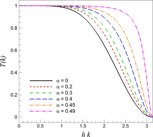
The free parameter, $\alpha$, which is in the range $|\alpha |<0.5$, determines the filtering properties, with high values of $\alpha$ yielding less dissipative results. It is easy to verify that the value of $\alpha =0.5$ yields back the unfiltered quantity of interest. A modified wavenumber analysis yields a transfer function, T(k), which correlates the Fourier coefficients of the filtered variable to those of the unfiltered variable in the Fourier domain, as follows (San, 2016):(32) $$\begin{array}{c}\hfill T(k)=\frac{a_0+a_{1}cos(hk)+a_{2}cos(2hk)+a_{3}cos(3hk)}{1+2\alpha cos(hk)},\end{array}$$(32)

where k is the wavenumber and h is the grid spacing. The transfer function of the Padé filter for different values of $\alpha$ are plotted in Figure 1, showing that the Padé filter remains close to unity over a wide range of wavenumbers, resulting in minimal dissipation over resolved inertial scales. Also, another characteristic of the compact Padé filter is that the maximum attenuation happens for the largest wavenumber (i.e. T(k) goes zero when k becomes the grid cut-off wavenumber). As a special case in Equation (30(30) $$\begin{array}{c}\hfill \alpha {\overline{\tilde{f}}}_{j-1}+{\overline{\tilde{f}}}_j+\alpha {\overline{\tilde{f}}}_{j+1}=\sum _{s=0}^3\frac{a_s}{2}({\tilde{f}}_{j-s}+{\tilde{f}}_{j+s}),\end{array}$$(30) ), where the free parameter $\alpha =0$, we obtain the following discrete filter:(33) $$\begin{array}{c}\hfill {\overline{\tilde{f}}}_j=\frac{1}{64}({\tilde{f}}_{j-3}-6{\tilde{f}}_{j-2}+15{\tilde{f}}_{j-1}+44{\tilde{f}}_j+15{\tilde{f}}_{j+1}-6{\tilde{f}}_{j+2}+{\tilde{f}}_{j+3}).\end{array}$$(33)

We also note that Equation (33(33) $$\begin{array}{c}\hfill {\overline{\tilde{f}}}_j=\frac{1}{64}({\tilde{f}}_{j-3}-6{\tilde{f}}_{j-2}+15{\tilde{f}}_{j-1}+44{\tilde{f}}_j+15{\tilde{f}}_{j+1}-6{\tilde{f}}_{j+2}+{\tilde{f}}_{j+3}).\end{array}$$(33) ) is also called sixth-order binomial smoothing filter and its transfer function can be written as Jahne (1997)(34) $$\begin{array}{c}\hfill T(k)=1-(1-\frac{1}{2}(1+cos(hk)){)}^3.\end{array}$$(34)

Unless otherwise stated, we use Equation (33(33) $$\begin{array}{c}\hfill {\overline{\tilde{f}}}_j=\frac{1}{64}({\tilde{f}}_{j-3}-6{\tilde{f}}_{j-2}+15{\tilde{f}}_{j-1}+44{\tilde{f}}_j+15{\tilde{f}}_{j+1}-6{\tilde{f}}_{j+2}+{\tilde{f}}_{j+3}).\end{array}$$(33) ) in our numerical assessments.

Figure 1. Transfer functions of the sixth-order compact Padé filters for various free filtering parameters.

3. Numerical schemes

In this study, we use the method of lines procedure by utilizing an explicit Runge–Kutta scheme for time integration. Specifically, a sixth-order compact central difference and a third-order optimal Runge–Kutta schemes are used for the spatial and temporal discretizations, respectively. In the compact central difference scheme, the first derivative of any function f on a collocated finite difference grid can be computed as follows (Lele, 1992):(35) $$\begin{array}{c}\hfill \frac{1}{3}{f}_{j-1}^{\prime }+f_j^{\prime }+\frac{1}{3}{f}_{j+1}^{\prime }=\frac{14}{9}\frac{f_{j+1}-f_{j-1}}{2h}+\frac{1}{9}\frac{f_{j+2}-f_{j-2}}{4h},\end{array}$$(35)

where h is the uniform grid spacing and superscript prime denotes the first derivative (i.e. $f^{\prime }=\frac{\partial f}{\partial x}$). Here, Equation (35(35) $$\begin{array}{c}\hfill \frac{1}{3}{f}_{j-1}^{\prime }+f_j^{\prime }+\frac{1}{3}{f}_{j+1}^{\prime }=\frac{14}{9}\frac{f_{j+1}-f_{j-1}}{2h}+\frac{1}{9}\frac{f_{j+2}-f_{j-2}}{4h},\end{array}$$(35) ) provides a sixth-order tridiagonal scheme which can be solved efficiently using the Thomas algorithm (1992). Similarly, the compact sixth-order centered scheme for the second derivative is given by(36) $$\begin{array}{cc}\hfill \frac{2}{11}{f}_{j-1}^{″}+f_j^{″}+\frac{2}{11}{f}_{j+1}^{″}& =\frac{12}{11}\frac{f_{j+1}-2f_j+f_{j-1}}{h^2}+\frac{3}{11}\frac{f_{j+2}-2f_j+f_{j-2}}{4h^2},\hfill \end{array}$$(36)

where superscript double prime denotes the second derivative (i.e. $f^{″}=\frac{{\partial }^{2}f}{\partial x^2}$).

In the method of lines, a system of semi-discrete ordinary differential equations is obtained after the spatial discretization of the governing equations. For example, the discrete version of Equation (4(4) $$\begin{array}{c}\hfill \frac{\partial \overline{\tilde{u}}}{\partial t}+\frac{1}{2}\frac{\partial (\overline{\tilde{u}}\overline{\tilde{u}})}{\partial x}=\nu \frac{{\partial }^2\overline{\tilde{u}}}{\partial x^2}+g,\end{array}$$(4) ) can be written as(37) $$\begin{array}{c}\hfill \frac{d{\overline{\tilde{u}}}_j}{\mathit{dt}}=\mathrm{\pounds }({\overline{\tilde{u}}}_j),\end{array}$$(37)

where $\mathrm{\pounds }({\overline{\tilde{u}}}_j)$ is the discrete operator for the nonlinear, linear, and SGS terms. We assume that the numerical approximation for time level n is known, and we seek the numerical approximation for time level $n+1$, after the time step $\mathrm{\Delta }t$. The optimal third-order accurate total variation diminishing Runge–Kutta scheme is then given as follows (Gottlieb & Shu, 1998):(38) $$\begin{array}{cc}\hfill {\overline{\tilde{u}}}_j^{(1)}& ={\overline{\tilde{u}}}_j^{(n)}+\mathrm{\Delta }t\mathrm{\pounds }({\overline{\tilde{u}}}_j^{(n)}),\hfill \\ \hfill {\overline{\tilde{u}}}_j^{(2)}& =\frac{3}{4}{\overline{\tilde{u}}}_j^{(n)}+\frac{1}{4}{\overline{\tilde{u}}}_j^{(1)}+\frac{1}{4}\mathrm{\Delta }t\mathrm{\pounds }({\overline{\tilde{u}}}_j^{(1)}),\hfill \\ \hfill {\overline{\tilde{u}}}_j^{(n+1)}& =\frac{1}{3}{\overline{\tilde{u}}}_j^{(n)}+\frac{2}{3}{\overline{\tilde{u}}}_j^{(2)}+\frac{2}{3}\mathrm{\Delta }t\mathrm{\pounds }({\overline{\tilde{u}}}_j^{(2)}).\hfill \end{array}$$(38)

4. Results

In this section, we present our results for two test cases: (i) the shock formation problem initiated by a single-mode sine wave, $u(x,0)=sin(x)$, and (ii) the decaying Burgers turbulence problem initiated by a specified energy spectrum considering the 64 sample initial conditions associated with randomly generated phases. Further details on the initial energy spectrum can be found in San (2016). Both problems are considered in a domain of $x\in [0,2\pi ]$ with periodic boundary conditions using $\nu =5\times {10}^{-4}$. Time integration for our discrete system is carried out using a third-order accurate total variation diminishing Runge–Kutta scheme with $\mathrm{\Delta }t=1\times {10}^{-5}$, and the sixth-order central compact difference schemes are used for the spatial discretizations to ensure a minimal numerical error.

4.1. Single-mode sine wave simulations

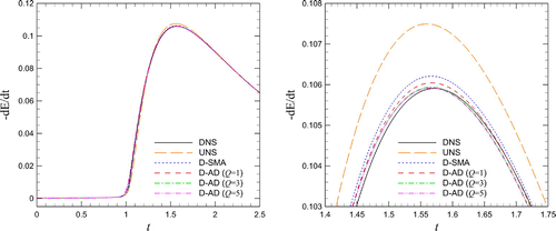
Figure 2 shows simulation results for the canonical problem initiated by the single-mode sine wave. The time evolution of the wave propagation obtained by a DNS computation on the resolution of $N=32768$ is illustrated in Figure 2(a) demonstrating the shock formation at a time approximately equal to 1.55. After the shock has developed at the time $t=2.5$, results performed by the under-resolved numerical simulation (UNS) where no-turbulence model is used, and the dynamic Smagorinsky (D-SMA) models are presented in Figure 2(b) and (c), respectively. These sets of results are obtained using resolutions of $N=512$, $N=1024$, and $N=2048$, and it is shown that grid-to-grid oscillations are apparent particular for the coarsest grid. On the other hand, as shown in Figure 2(d–f), the proposed dynamic AD (D-AD) model yields substantially better results with the damping of grid-to-grid oscillations by increasing Q, the order of Van Cittert iteration, which can also be seen from Figure 3 demonstrating the total dissipation rate $-dE/dt$ where $E=\int E(k)dk$ is the total kinetic energy. Figure 3 also demonstrates that the peak value of the dissipation rate agrees well with the DNS data.

Figure 2. Conservative formulation results for solving the Burgers equation initiated by the single-mode sine wave: (a) time evolution by DNS with resolution of $N=32768$; (b) under-resolved numerical simulation (UNS); (c) dynamic Smagorinsky model (D-SMA); and (d–f) the proposed dynamic AD model (D-AD) with various orders of Q. In (b–f), we present the final snapshots at time $t=2.5$ using resolutions of 512, 1024, and 2048 where the results for 512 and 1024 resolutions are shifted in the x-axis for the purpose of illustration.

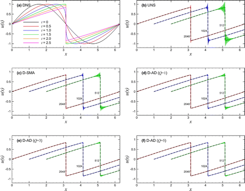
Figure 3. Conservative formulation for the shock formation problem initiated by a single-mode sine wave using 512 grid points: a comparison for the time evolution of the dissipation rate (left) and its close-up for local enlargement (right).

The nonlinear term given in Equation (1(1) $$\begin{array}{c}\hfill \frac{\partial u}{\partial t}+\frac{\partial (u^2/2)}{\partial x}=\nu \frac{{\partial }^{2}u}{\partial x^2},\end{array}$$(1) ) can be also written in the skew-symmetric form, Ritchmyer and Morton (1967), Jameson (2008), leading to(39) $$\begin{array}{c}\hfill \frac{1}{2}\frac{\partial (uu)}{\partial x}=\frac{1}{3}u\frac{\partial u}{\partial x}+\frac{1}{3}\frac{\partial (uu)}{\partial x}.\end{array}$$(39)

It has been well known that the discrete version of these formulations yields slightly different results.

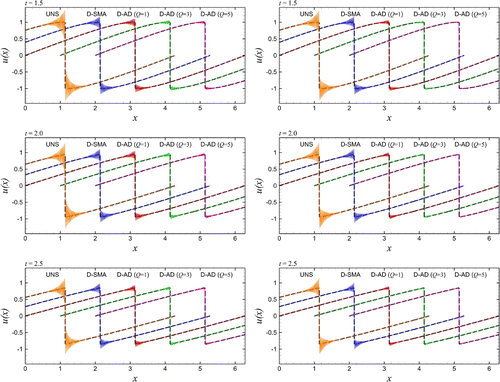
To analyze the effect of the formulation, we perform the same analysis using the skew-symmetric form for the nonlinear term. Having parameters identical to those used in Figures 2 and 3 for the conservative form, Figures 4 and 5 illustrate the results obtained by the skew-symmetric form. Further comparisons are shown in Figure 6 for energy spectra and in Figure 7 for velocity fields. Although similar conclusions can be made from these observations regarding the closure modeling performance of the proposed framework, we can easily see that the skew-symmetric formulation yields slightly better results due to its discrete conservation properties. A first conclusion from these results suggests that the proposed D-AD model is more dissipative than the D-SMA model and reduces grid-to-grid oscillations even for considerably coarse grids. It is also evident on examinations of Figure 7 that the shock capturing property of the proposed D-AD model is superior to the D-SMA model.

Figure 4. Skew-symmetric formulation simulation results for solving the Burgers equation initiated by the single-mode sine wave: (a) time evolution by DNS with resolution of $N=32768$; (b) under-resolved numerical simulation (UNS); (c) dynamic Smagorinsky model (D-SMA); and (d–f) the proposed dynamic AD model (D-AD) with various orders of Q. In (b–f), we present the final snapshots at time $t=2.5$ using resolutions of 512, 1024, and 2048 where the results for 512 and 1024 resolutions are shifted in the x-axis for the purpose of illustration.

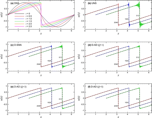
Figure 5. Skew-symmetric formulation for the shock formation problem initiated by a single-mode sine wave using 512 grid points: a comparison for the time evolution of the dissipation rate (left) and its close-up for local enlargement (right).

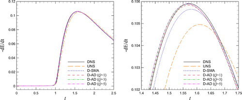
Figure 6. A comparison of energy spectra for $N=512$ resolution results at time $t=2.5$ obtained by the conservative (left) and skew-symmetric (right) formulations for the shock formation problem initiated by a single-mode sine wave.

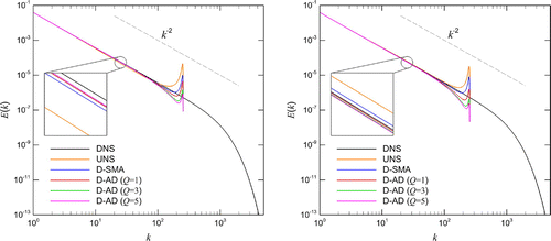
Figure 7. Intercomparison of $N=512$ resolution results for solving the Burgers equation initiated by the single-mode sine wave using the conservative formulation (left column) and the skew-symmetric formulation (right column). Note that the simulation results for UNS, D-SMA, D-AD ($Q=3$), and D-AD ($Q=5$) are shifted in x-axis for the purpose of illustration.

4.2. Decaying Burgers turbulence simulations

Next, we present our results for the Burgers turbulence problem in a periodic domain of $x\in [0,2\pi ]$. We solve 64 different cases generated from the following initial energy spectrum(40) $$\begin{array}{c}\hfill E(k)=\frac{2}{3\sqrt{\pi }}\frac{k^4}{k_0^5}{e}^{-{(k/k_0)}^2},\end{array}$$(40)

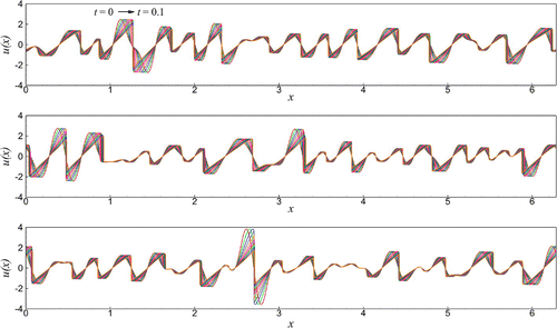
where $k_0=10$. Figure 8 illustrates the solution fields for three of them obtained using DNS with a resolution of $N=32768$. We note that each simulation is obtained using the same initial energy spectrum with randomly assigned phase distributions (i.e. in order to generate different initial conditions in physical space). Figure 9(a) illustrates the time evolution of the decaying Burgers turbulence based upon the ensemble average of 64 sample fields, obtained by DNS with a resolution of $N=32768$. Figure 9(b) shows the energy spectra at $t=0.05$ for DNS and UNS computations for different resolutions demonstrating the ideal $k^{-2}$ scaling at inertial range. It is clear from figure that the resolution of $N=32768$ yields DNS data resolving all associated shock scales at $\nu =5\times {10}^{-4}$. One must note that $t=0.05$ corresponds approximately to the time for the maximum dissipation rate of the problem. The energy pile-up close to grid cut-off scale is also evident at lower resolutions.

Figure 8. Space–time solutions of the Burgers equation using three different initial conditions generated from Equation (40(40) $$\begin{array}{c}\hfill E(k)=\frac{2}{3\sqrt{\pi }}\frac{k^4}{k_0^5}{e}^{-{(k/k_0)}^2},\end{array}$$(40) ).

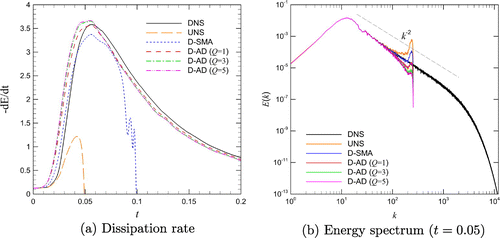
In Figure 10, we present our LES analysis using the coarsest resolution of $N=512$ illustrating the time evolution of the total dissipation rate and energy spectra at time $t=0.05$. Results obtained by DNS, UNS, and the dynamic Smagorinsky (D-SMA) model are also included for the purpose of comparison. It is shown that the proposed dynamic model yields a dissipation rate with considerably higher accuracy and the energy pile-up can be effectively eliminated by increasing Q. It is also evident on careful examination of Figure 10 that the overall accuracy of the proposed scheme is fairly good over the entire simulation time. However, the UNS and the dynamic Smagorinsky (D-SMA) models cannot capture the physics beyond $t=0.05$ due to accumulation of grid-to-grid oscillations. In a manner similar to the previous test case, increasing Q yields an improved approximation to the representation of the SFS interactions. This implies that more dissipative behavior can be obtained using a higher order Van Cittert iterative procedure, which would be crucial for solving LES equations on very coarse grid resolutions. We also found that results are negligibly improved by increasing the order of Van Cittert iterations beyond $Q=5$.

Figure 9. Time evolution of the energy spectrum for the Burgers turbulence problem based upon the ensemble average of 64 sample fields obtained by DNS ($N=32768$) (left), and a comparison of energy spectra at time $t=0.05$ obtained by various spatial resolutions ranging from $N=512$ to $N=32768$ (right).

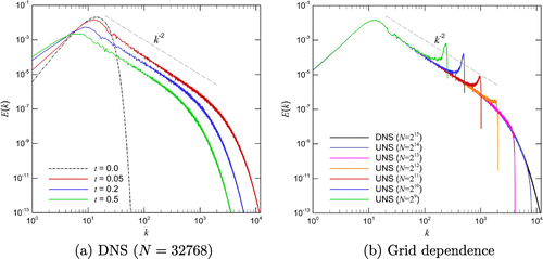
Figure 10. Results for the SGS modeling of the Burgers turbulence problem obtained using $N=512$ resolution with the conservative formulation of the nonlinear term: time evolution of the total dissipation rate (left) and energy spectra at time $t=0.05$ (right).

To analyze the discrete formulation effect, we perform the same analysis using the skew-symmetric form for the nonlinear term. Utilizing parameters and initial conditions identical to those used for Figures 9–12 illustrate the results obtained by the skew-symmetric form. It is noted that the same resolving performance is obtained for the finest resolution, which can be considered as a verification of its DNS characteristics at $N=32768$. As discussed earlier, we can easily see that the skew-symmetric formulation yields slightly better results due to its discrete conservation properties. In the skew-symmetric formulation, all coarse grid simulations yield stable numerical solutions for all time evolutions for the decaying Burgers turbulence cases. However, it is clear that the D-AD model predicts the peak dissipation rate better.

Figure 11. Time evolution of the energy spectrum for the Burgers turbulence problem based upon the ensemble average of 64 sample fields obtained by DNS ($N=32768$) (left), and energy spectra at time $t=0.05$ obtained by various spatial resolutions ranging from $N=512$ to $N=32768$ (right).

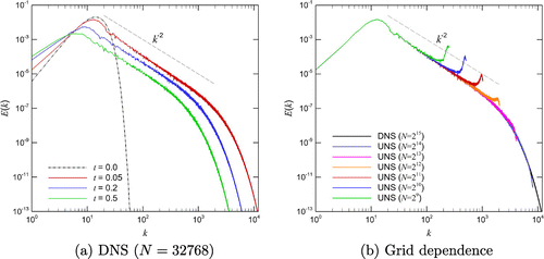
Figure 12. Results for the SGS modeling of the Burgers turbulence problem obtained using $N=512$ resolution with the skew-symmetric formulation of the nonlinear term: time evolution of the total dissipation rate (left) and energy spectra at time $t=0.05$ (right).

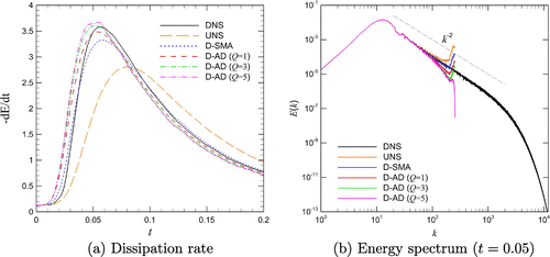
Figure 13. A sensitivity analysis with respect to the free filtering parameter $\alpha$ for solving the Burgers turbulence problem and showing the energy spectra at time $t=0.05$ using the conservative formulation on $N=512$ resolution.

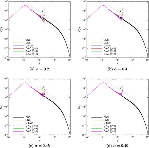
Figure 14. A sensitivity analysis with respect to the free filtering parameter $\alpha$ for solving the Burgers turbulence problem and showing the energy spectra at time $t=0.05$ using the skew-symmetric formulation on $N=512$ resolution.

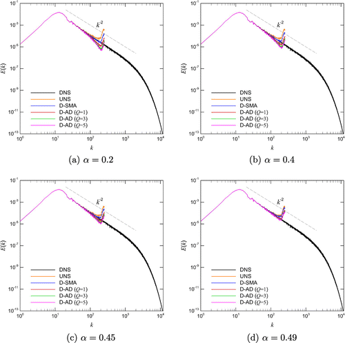
It is also shown that the proposed model yields more dissipative results. It follows a similar trend that we observed in the case of the single-mode sine wave experiments in which we obtain more dissipative results for higher order Q. This can be explained in such a way that an increase in the order Q yields an increase of the estimated $C_S$ value. An examination of energy spectra plots given in Figure 12 reveals that the D-SMA yields a longer inertial range compared to the D-AD. This can be explained by the use of relatively dissipative behavior of the low-pass filter given by Equation (33(33) $$\begin{array}{c}\hfill {\overline{\tilde{f}}}_j=\frac{1}{64}({\tilde{f}}_{j-3}-6{\tilde{f}}_{j-2}+15{\tilde{f}}_{j-1}+44{\tilde{f}}_j+15{\tilde{f}}_{j+1}-6{\tilde{f}}_{j+2}+{\tilde{f}}_{j+3}).\end{array}$$(33) ). Therefore, a sensitivity analysis with respect to the free filtering parameter $\alpha$ is also presented in Figure 13. As shown here less dissipative results can be obtained using a less dissipative filter (i.e. increasing $\alpha$). Here, we note that larger inertial range can be obtained by increasing $\alpha$ value in the D-AD model. It can also be seen that UNS data can be recovered when $\alpha \to 0.5$. We emphasize that a-posteriori results of D-SMA and D-AD models depend on the free filtering parameters, underlying numerical scheme, convective term formulation, and computational resolution. Using the same filtering kernel and the same discrete method, our numerical assessments show that the D-SMA performs better for capturing the larger inertial range since the D-AD model acts more dissipative. On the other hand, the D-AD performs better to eliminate grid-to-grid oscillations and provide more stable results for coarser grids due to the its more dissipative behavior. Furthermore, the level of dissipation can be controlled by the free filtering parameter.

5. Conclusion

We propose a simplified dynamic framework for SGS modeling of LES of turbulent flows based upon the use of AD process to compute the Smagorinsky constant self-adaptively from the resolved flow quantities. Our proposed model replaces the test filtering procedure of the standard dynamic model with the AD procedure. Although the presentation of the model is given using the Burgers equation, its generalization to the Navier–Stokes equations is straightforward. Our numerical assessments for solving the single-mode sine wave and the Burgers turbulence problems show that the proposed approach could represent a viable tool for subgrid scale parametrization of turbulent flows by combining the AD process with an eddy viscosity model. Since we consider only the SFS portion of the residual interactions when computing the free modeling parameter, the AD procedure provides for a more dissipative eddy viscosity model than the classical test filtering approach and results in a more stable behavior reducing the grid-to-grid oscillations in coarse grid central scheme-based LES computations.

Acknowledgements

This work was completed utilizing the High Performance Computing Center facilities of Oklahoma State University at Stillwater.

Additional information

Funding

The authors received no direct funding for this research.

Notes on contributors

Romit Maulik

Romit Maulik is a PhD candidate at the School of Mechanical and Aerospace Engineering at Oklahoma State University (OSU). He received his BSc degree from Birla Institute of Technology and MSc degree from the School of Mechanical and Aerospace Engineering at OSU. He is interested in mathematical modeling of turbulent flows and machine learning applications in fluid dynamics.

Omer San

Omer San is an assistant professor at the School of Mechanical and Aerospace Engineering at OSU. He received his PhD in Engineering Mechanics from Virginia Tech in 2012. He held two postdoctoral research positions, first in the Interdisciplinary Center for Applied Mathematics (ICAM) at Virginia Tech from 2012–’14, then from 2014–’15 in the Center for Shock Wave-processing of Advanced Reactive Materials (C-SWARM) at the University of Notre Dame, Indiana. Since 2015, he has been with the faculty of the School of Mechanical and Aerospace Engineering at OSU-Stillwater. His research interests include multiscale modeling and simulation, fluid dynamics, and high performance computing.

References

- Adams, N. A., & Stolz, S. (2002). A subgrid-scale deconvolution approach for shock capturing. Journal of Computational Physics, 178(2), 391–426.
- Berland, J., Lafon, P., Daude, F., Crouzet, F., Bogey, C., & Bailly, C. (2011). Filter shape dependence and effective scale separation in large-eddy simulations based on relaxation filtering. Computers & Fluids, 47(1), 65–74.
- Berselli, L. C., Iliescu, T., & Layton, W. J. (2006). Mathematics of large eddy simulation of turbulent flows. New York, NY: Springer-Verlag.
- Biemond, J., Lagendijk, R. L., & Mersereau, R. M. (1990). Iterative methods for image deblurring. Proceedings of the IEEE, 78(5), 856–883.
- Bogey, C., & Bailly, C. (2004). A family of low dispersive and low dissipative explicit schemes for flow and noise computations. Journal of Computational Physics, 194(1), 194–214.
- Bogey, C., & Bailly, C. (2006a). Computation of a high Reynolds number jet and its radiated noise using large eddy simulation based on explicit filtering. Computers & Fluids, 35(10), 1344–1358.
- Bogey, C., & Bailly, C. (2006b). Large eddy simulations of transitional round jets: Influence of the Reynolds number on flow development and energy dissipation. Physics of Fluids, 18(6), 065101.
- Boris, J. P., Grinstein, F. F., Oran, E. S., & Kolbe, R. L. (1992). New insights into large eddy simulation. Fluid Dynamics Research, 10(4–6), 199–228.
- Bouffanais, R., Deville, M. O., & Leriche, E. (2007). Large-eddy simulation of the flow in a lid-driven cubical cavity. Physics of Fluids, 19(5), 055108.
- Bull, J. R., & Jameson, A. (2016). Explicit filtering and exact reconstruction of the sub-filter stresses in large eddy simulation. Journal of Computational Physics, 306, 117–136.
- Carati, D., Winckelmans, G. S., & Jeanmart, H. (2001). On the modelling of the subgrid-scale and filtered-scale stress tensors in large-eddy simulation. Journal of Fluid Mechanics, 441, 119–138.
- De Stefano, G., & Vasilyev, O. V. (2002). Sharp cutoff versus smooth filtering in large eddy simulation. Physics of Fluids, 14(1), 362–369.
- Dunca, A. A. (2011). On the existence of global attractors of the approximate deconvolution models of turbulence. Journal of Mathematical Analysis and Applications, 389(2), 1128–1138.
- Dunca, A. A., & Epshteyn, Y. (2006). On the Stolz-Adams deconvolution model for the large-eddy simulation of turbulent flows. SIAM Journal on Mathematical Analysis, 37(6), 1890–1902.
- Dunca, A. A., & Lewandowski, R. (2014). Error estimates in approximate deconvolution models. Communications in Mathematical Sciences, 12(4), 757–778.
- Falkovich, G., & Sreenivasan, K. R. (2006). Lessons from hydrodynamic turbulence. Physics Today, 59(4), 43–49.
- Fauconnier, D., De Langhe, C., & Dick, E. (2009). A family of dynamic finite difference schemes for large-eddy simulation. Journal of Computational Physics, 228(6), 1830–1861.
- Galperin, B., & Orszag, S. A. (1993). Large eddy simulation of complex engineering and geophysical flows. New York: Cambridge University Press.
- Germano, M. (1986). Differential filters for the large eddy numerical simulation of turbulent flows. Physics of Fluids, 29, 1755–1756.
- Germano, M. (2009). A new deconvolution method for large eddy simulation. Physics of Fluids, 21, 045107.
- Germano, M. (2015). The similarity subgrid stresses associated to the approximate Van Cittert deconvolutions. Physics of Fluids, 27(3), 035111.
- Germano, M., Piomelli, U., Moin, P., & Cabot, W. H. (1991). A dynamic subgrid-scale eddy viscosity model. Physics of Fluids, 3, 1760–1765.
- Gottlieb, S., & Shu, C. W. (1998). Total variation diminishing Runge-Kutta schemes. Mathematics and Computers, 67(221), 73–85.
- Gullbrand, J., & Chow, F. K. (2003). The effect of numerical errors and turbulence models in large-eddy simulations of channel flow, with and without explicit filtering. Journal of Fluid Mechanics, 495(1), 323–341.
- Habisreutinger, M. A., Bouffanais, R., Leriche, E., & Deville, M. O. (2007). A coupled approximate deconvolution and dynamic mixed scale model for large-eddy simulation. Journal of Computational Physics, 224(1), 241–266.
- Jahne, B. (1997). Digital image processing: Concepts, algorithms, and scientific aplications. Berlin, Heildelberg: Springer-Verlag.
- Jameson, A. (2008). The construction of discretely conservative finite volume schemes that also globally conserve energy or entropy. Journal of Scientific Computing, 34(2), 152–187.
- Jordan, S. A., & Ragab, S. A. (1996). A large-eddy simulation of the shear-driven cavity flow using dynamic modeling. International Journal of Computational Fluid Dynamics, 6(4), 321–335.
- Layton, W. (2016). Energy dissipation in the Smagorinsky model of turbulence. Applied Mathematics Letters, 59, 56–59.
- Layton, W., & Lewandowski, R. (2006). Residual stress of approximate deconvolution models of turbulence. Journal of Turbulence, 7, 1–21.
- Layton, W., & Neda, M. (2007). A similarity theory of approximate deconvolution models of turbulence. Journal of Mathematical Analysis and Applications, 333(1), 416–429.
- Layton, W. J., & Rebholz, L. (2012). Approximate deconvolution models of turbulence: analysis, phenomenology and numerical analysis. Berlin: Springer-Verlag.
- Lele, S. K. (1992). Compact finite difference schemes with spectral-like resolution. Journal of Computational Physics, 103(1), 16–42.
- Lesieur, M., & Metais, O. (1996). New trends in large-eddy simulations of turbulence. Annual Review of Fluid Mechanics, 28(1), 45–82.
- Lilly, D. K. (1992). A proposed modification of the Germano subgrid-scale closure method. Physics of Fluids, 4, 633–635.
- Love, M. D. (1980). Subgrid modelling studies with Burgers’ equation. Journal of Fluid Mechanics, 100(01), 87–110.
- Lund, T. S. (2003). The use of explicit filters in large eddy simulation. Computers & Mathematics with Applications, 46(4), 603–616.
- Mathew, J., Foysi, H., & Friedrich, R. (2006). A new approach to LES based on explicit filtering. International Journal of Heat and Fluid Flow, 27(4), 594–602.
- Mathew, J., Lechner, R., Foysi, H., Sesterhenn, J., & Friedrich, R. (2003). An explicit filtering method for large eddy simulation of compressible flows. Physics of Fluids, 15(8), 2279–2289.
- Maulik, R., & San, O. (2017a). A dynamic subgrid-scale modeling framework for boussinesq turbulence. International Journal of Heat and Mass Transfer, 108, 1656–1675.
- Maulik, R., & San, O. (2017b). A novel dynamic framework for subgrid scale parametrization of mesoscale eddies in quasigeostrophic turbulent flows. Computers & Mathematics with Applications, 74, 420–445.
- Maulik, R., & San, O. (2017c). A stable and scale-aware dynamic modeling framework for subgrid-scale parameterizations of two-dimensional turbulence. Computers & Fluids, 158, 11–38.
- Meneveau, C., & Katz, J. (2000). Scale-invariance and turbulence models for large-eddy simulation. Annual Review of Fluid Mechanics, 32(1), 1–32.
- Mullen, J. S., & Fischer, P. F. (1999). Filtering techniques for complex geometry fluid flows. Communications in Numerical Methods in Engineering, 15(1), 9–18.
- Najafi-Yazdi, A., Najafi-Yazdi, M., & Mongeau, L. (2015). A high resolution differential filter for large eddy simulation: Toward explicit filtering on unstructured grids. Journal of Computational Physics, 292, 272–286.
- Najjar, F. M., & Tafti, D. K. (1996). Study of discrete test filters and finite difference approximations for the dynamic subgrid-scale stress model. Physics of Fluids, 8, 1076–1088.
- Orszag, S. A. (1971). On the elimination of aliasing in finite-difference schemes by filtering high-wavenumber components. Journal of the Atmospheric Sciences, 28(6), 1074–1074.
- Piomelli, U. (1999). Large-eddy simulation: achievements and challenges. Progress in Aerospace Sciences, 35(4), 335–362.
- Press, W., Teukolsky, S., Vetterling, W., & Flannery, B. (1992). Numerical recipes in FORTRAN: The art of scientific computing. New York: Cambridge University Press.
- Pruett, C. D., & Adams, N. A. (2000). A priori analyses of three subgrid-scale models for one-parameter families of filters. Physics of Fluids, 12, 1133–1142.
- Rebholz, L. G. (2007). Conservation laws of turbulence models. Journal of Mathematical Analysis and Applications, 326(1), 33–45.
- Ritchmyer, R. D., & Morton, K. W. (1967). Difference methods for initial-value problems. New York: Interscience.
- Sagaut, P. (2006). Large eddy simulation for incompressible flows: an introduction. New York: Springer-Verlag.
- Sagaut, P., & Grohens, R. (1999). Discrete filters for large eddy simulation. International Journal for Numerical Methods in Fluids, 31(8), 1195–1220.
- San, O. (2016). Analysis of low-pass filters for approximate deconvolution closure modeling in one-dimensional decaying Burgers turbulence. International Journal of Computational Fluid Dynamics, 30, 20–37.
- Sarghini, F., Piomelli, U., & Balaras, E. (1999). Scale-similar models for large-eddy simulations. Physics of Fluids, 11(6), 1596–1607.
- Smagorinsky, J. (1963). General circulation experiments with the primitive equations. I. The basic experiments. Monthly Weather Review, 91(3), 99–164.
- Smagorinsky, J. (1993). Some historical remarks on the use of nonlinear viscosities. In B. Galperin & S. A. Orszag (Eds.), Large eddy simulation of complex engineering and geophysical flows (pp. 3–36). New York: Cambridge University Press.
- Stanculescu, I. (2008). Existence theory of abstract approximate deconvolution models of turbulence. Annali dell’Universita di Ferrara, 54(1), 145–168.
- Stolz, S., & Adams, N. A. (1999). An approximate deconvolution procedure for large-eddy simulation. Physics of Fluids, 11, 1699–1701.
- Stolz, S., Adams, N. A., & Kleiser, L. (2001). An approximate deconvolution model for large-eddy simulation with application to incompressible wall-bounded flows. Physics of Fluids, 13, 997–1015.
- Vasilyev, O. V., Lund, T. S., & Moin, P. (1998). A general class of commutative filters for LES in complex geometries. Journal of Computational Physics, 146(1), 82–104.
- Zang, Y., Street, R. L., & Koseff, J. R. (1993). A dynamic mixed subgrid-scale model and its application to turbulent recirculating flows. Physics of Fluids, 5(12), 3186–3196.