Determinants influencing Vietnam coffee exports

Abstract

This study investigates the impact levels of determinants on Vietnam’s coffee exports by applying the Spatial Gravity Model and panel data to consider the spatial dependence in the gravity model. The Spatial Gravity Model was employed to spatially examine influencing factors among trading partners by means of spatial econometric approaches, based on Vietnamese coffee export data for 20 countries from 2005 to 2019. The results reveal that the export of coffee products is influenced by many determinants such as the gross domestic product (GDP) of the importing country, population, exchange fluctuations, free trade agreement (FTA), non-tariff barriers to trade, and tax rate. Among these determinants, GDP growth and population growth have a positive impact on coffee exports. On the other hand, tariffs, non-tariff barriers and exchange rate variables are factors that negatively affect coffee exports. In addition, the distance between countries has a negative impact on exports overall.

Impact Statement

This study investigates the impact levels of determinants on Vietnam’s coffee exports by applying the Spatial Gravity Model and panel data to consider the spatial dependence in the gravity model. The Spatial Gravity Model was employed to spatially examine influencing factors among trading partners by means of spatial econometric approaches, based on Vietnamese coffee export data for 20 countries from 2005 to 2019. The results reveal that the export of coffee products is influenced by many determinants such as the gross domestic product (GDP) of the importing country, population, exchange fluctuations, free trade agreement (FTA), non-tariff barriers to trade, and tax rate.

Keywords:

• Spatial gravity model
• coffee
• export
• Vietnam

Reviewing Editor:

• Huifen (Helen) Cai, Middlesex University Business School, United Kingdom

Subjects:

• Econometrics
• International Economics
• Development Economics

JEL CLASSIFICATION CODES:

• C21
• F1

1. Introduction

Coffee is an important export crop and accounts for a large proportion of Vietnam’s agricultural export turnover. According to preliminary data reported by Vietnam Customs in 2019, coffee exports reached to 1,653,265 tons, with a total export value of 2.85 billion USD, accounting for 27% of total export value. In recent years, the increasing trend and demand for coffee in the world has drawn attention to the importance of coffee products, providing an opportunity and a new growth engine for coffee exports in Vietnam. Therefore, the Vietnamese government has participated in various coffee-export support projects including joining the European-Vietnam Free Trade Agreement (EVFTA). This agreement has strongly supported Vietnam’s coffee exports to Europe when the tax was eliminated for all raw or processed coffee products specifically raw coffee (decreased from 7–11% to 0%), processed coffees (down from 9–12% to 0%) which offered competitive advantages to Vietnamese coffee.

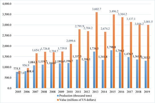
Moreover, the accessibility to the World Trade Organization (WTO), and other international, and regional organizations has created a large market for the Vietnamese coffee industry. The policy of free trade and market expansion in recent years has brought into play the strength of all economic sectors in coffee production and trading. The connection between domestic and foreign markets created favorable conditions for the coffee industry to expand its consumption channels domestically and internationally. In recent years, the largest coffee export markets of Vietnam are Germany, the United States, Italy, Spain and Japan. These countries account for an average of 75.65% of the total coffee export turnover of Vietnam. Which, Germany is Vietnam’s largest coffee export market, accounting for 24.3% of total coffee export value. Italy, secondly, accounted for 15.5%. Spain, thirdly, accounted for 13.67%. Finally, Japan accounted for 9.18%. The volume of coffee exported from Vietnam from 2005 to 2019 has fluctuated. During 2005, 775.5 thousand tonnes of coffee were exported (specifically, it reached 775.5 thousand tonnes in 2005), which resulted in an exported value of about 827 million dollars.

From 2006 to 2011, the volume of Vietnamese coffee exports tended to increase gradually compared to 2005. From 2012 to 2014, the volume of coffee exports began to show a decrease. Vietnam’s coffee exports have been constantly fluctuating from 2015 to 2019 with a decreasing export volume ever since. Although the Vietnamese government has promoted and implemented many projects to support coffee exports, in 2019 coffee exports totaled 1,303.2 thousand tons, a decrease of 12.09% in volume and a 21.28% decrease in price compared to exports in 2018. Coffee exports in 2018 totaled 1,361.8 thousand tons, down 11.92% in volume and 19.28% in price compared to 2017. Coffee export volume in 2017 reached 1,476.5 thousand tons, worth 3,137.2 million USD, down 19% in volume and 2.7% in price compared to 2016 (See Figure 1). Therefore, the analysis of factors affecting Vietnam’s coffee exports will be important in identifying and predicting the fluctuations of exports. Vietnam is the second largest coffee producer and exporter in the world. However, 90% of Vietnamese coffee exports are in raw form: coffee beans, which have low-value exports.

Figure 1. Coffee exports of Vietnam for the period 2005–2019.

Source: General Department of Vietnam Customs in 2019.

The main factors affecting Vietnam’s coffee exports, that have caused a sharp decline in coffee exports in recent years, are economic conditions, changes in trading partners, exchange rate fluctuations, Free Trade Agreements (FTAs), tax rates, non-tariff barriers, and others. However, studies on the coffee trade that comprehensively consider factors affecting Vietnam’s coffee exports have not been researched thoroughly.

2. Literature review

Numerous works go further into research and analysis on the elements influencing Vietnam’s coffee exports, but only a small number of them use gravity models to make coffee exports. Pham (2018) uses a gravity model to assess the market size, economy size, population, and GDP determinants influencing Vietnam’s coffee exports to the Chinese market. However, these studies do not account for the spatial dependence or spillover effect of trade flows between countries when using gravity models. The study by Do (2019), which also used the gravity model, examined and identified the currency rate as one of the factors influencing Vietnam’s coffee exports to nations in the European Union from 2010 to 2014. As a result, it is difficult to determine how the exchange rate would affect Vietnam’s exports of coffee. By using the real effective exchange rate, which is the weighted average of the proportion of coffee exports, computed through the price index of coffee, consumption, and GDP, this study will thus address the flaws of the prior study.

The study by Nguyen (2021) that investigates the elements affecting Vietnam’s coffee exports uses the gravity model; the research findings show that trade expenses are one of those aspects. These studies, however, did not pay particular attention to elements like tariffs and non-tariff barriers, which have recently emerged as a source of particular worry for nations. Bui (2020) estimated that the export volume of Vietnamese coffee and cocoa, which are the main export items to China, will increase by an average of 2.1% when the EVFTA, and ASEAN – China were signed. Research through the gravity model in the estimation of factors affecting coffee and cocoa exports showed that factors such as transit time, freight rates, exchange rates, WTO membership and FTA agreements have a strong influence on Vietnam’s coffee and cocoa exports. The research does, however, not include time-invariant variables, such as the distance between countries, because they pose a complete multicollinearity issue in the fixed-effects analysis. Instead, the distance-by-country analysis is carried out at a later level in the random effects model. The oil price gap variable, which is computed by looking at oil prices for the distances between ports that have been used, will be employed in this study to be more precise. Because the difference in oil prices among nations changes, it is possible to examine how distance between nations affects exports even in a fixed-effects model.

In recent years, studies investigating the factors affecting Vietnam’s coffee exports based solely on the gravity model have not focused on spatial distance. Research applying spatial gravity models to analyze factors affecting Vietnam’s coffee exports is currently too limited. There are very few studies focusing on macro factors such as GDP, geographical distance, exchange rates, etc. Therefore, this study analyzes the factors affecting Vietnam’s coffee exports using a spatial gravity model, using panel data to consider spatial dependence in the gravity model. From there, it helps managers make implications and management policies related to improving the output and quality of Vietnam’s coffee exports.

Rendleman and Vasinvarthana (2013) analyzed the impact of non-tariff barriers such as Hazard Analysis and Critical Control Points (HACCP) and The Bioterrorism Act on US agricultural imports employing variables distance, GDP, etc. The dependent variable used in the analysis is US agricultural imports and independent variables are based on Hazard Analysis and Critical Control Points (HACCP) which operated in the US in 1998 when bioterrorism laws went into effect and trading partners’ export volumes. The estimated results showed that Hazard Analysis and Critical Control Points (HACCP) and the Bioterrorism Act have a negative impact on US agricultural imports, but it is not statistically significant. However, the study using the gravity model did not take into account spatial dependence such as distance between countries.

A variety of analytical methods have been applied to analyze the influencing factors in coffee export, including the gravity model which was introduced as a theory of international trade. This model shows that the size of trade varies with GDP and the distance between the two countries. In addition, it is widely used to analyze the impact of free trade agreements, tax rates and non-tariff barriers on trade between countries.

Evenett and Keller (2002) evaluated that the gravity model is effective in explaining the bilateral relationship between the two countries. Nevertheless, previous studies have not explicitly examined the spatial dependence between trading partners. For example, transactions between certain trading partners can affect transactions between other exporting countries, and vice versa. In other words, export determinants such as exchange rate fluctuations, FTA agreements, tax rates and non-tariff barriers not only affect trading partners, but also other countries’ exports have a large share of trade. Therefore, both analysis of impacts between trading partners and spillover effects between trading partners should be included in the model and analysis.

Nguyen (2020) analyzed the factors that positively impact trade facilitation with the application of the spatial gravity model and showed that trade facilitation variables such as logistics and transportation infrastructure have a significant influence on bilateral trade. In addition, the results revealed that progress in the average export value of the neighbors of a trading partner has decreased the value of that trading partner’s exports which means that variables in the neighboring countries of a trading partner have a negative effect on the exports of both countries. However, by evaluating one-way trade patterns in terms of the gravity model, the study is restricted to the investigation of multinational trade patterns. As a result, this research integrates multi-country commerce, which is defined as a type of bilateral trade, to address the shortcomings of earlier research. Nguyen (2012) analyzed the tariff reduction of South Korea based on the trade diversion effect from imports of neighboring countries to imports from the US through the abolition of tariffs since the signing of the agreement Korea-US free trade agreement (FTA) estimated results based on space gravity model that the volume of trade between Korea and the US increased due to tariff reductions, whilst overall trade volume with neighboring countries decreased due to ripple effect.

Gautschi (1981) found that when the model is estimated without considering the influence of spatial factors between countries, the estimated coefficients of related variables will tend to be overestimated, making it impossible to guarantee the reliability of the overall estimate. In this regard, Anselin (1988) suggested that when estimating a model using spatial data such as country or region, the dependent variable or error of an individual country is correlated with the dependent variable or error observed in neighboring countries, this is called spatial dependence which is also known as spatial autocorrelation.

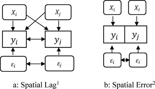
Figure 2 illustrates that the dependent variables or errors are spatially correlated. If spatial dependence is not considered, this violates the basic assumptions of econometrics concerning explanatory variables and errors. When estimates are made by using general regression, spatial autocorrelation will appear biased or inefficient. In terms of the spatial autocorrelation in the Gravity model, LeSage and Pace (2008), basic variables in the gravity model of the countries include GDP, population, production of analyzed commodities, etc. This is because the data is built into an artificial spatial unit called a border even though they tend to be interconnected. For example, the GDP and population of EU and NAFTA countries are influenced by the characteristics and proximity of neighboring countries; the socio-economic situation of neighboring countries and the mobility of the labor force between countries. For this reason, it is necessary to actively consider spatial influences when using gravity models, i.e. spatial dependence.

Figure 2. Two major types of autocorrelation spatial dependencies.

Source: LeSage (1999) Spatial Econometrics.

There are, however, very few domestic studies on gravity models that take into account spatial dependency (autocorrelation) or the spillover effect of trade flows between nations. There aren’t many studies that quantitatively examine the variables influencing Vietnam’s exports of coffee. To overcome the shortcomings of previous studies, this study will employ a spatial gravity model that takes spatial dependence into account. The objective is to gather, analyze, and function-analyze data. By utilizing a spatial gravity model to analyze the variables impacting Vietnam’s coffee exports, take note of the management policies connected to the enhancement of export output.

3. Theoretical framework and research methodology

3.1. Theoretical framework

The first gravity model was applied by Leibenstein and Tinbergen (1962). It is named the ‘gravity model’ like Isaac Newton’s Law of Gravity. The theory of the gravity model is derived from Newton’s law of gravitation to explain the flow of trade between two countries. Tinbergen’s application of gravity model reasoning to international trade analysis is shown in model (1) below, which means that the amount of trade between countries is directly proportional to the economic size of the countries and inversely proportional to the distance. (1) $$\frac{d{A}_i}{\mathit{\text{dt}}}=k_{\left(i+1\right)\to i}\text{*}{e}^{-\left(k_H\mathit{\text{*time}}\right)}\text{*}{A}_{\left(i+1\right)}‐\hspace{0.17em}{k}_{i\to \left(i-1\right)}\text{*}{e}^{-\left(k_H\mathit{\text{*time}}\right)}\text{*}{A}_i$$(1)

In model (1), $Y_{\mathit{\text{od}} }$ is the number of transactions between the origin (o) and the destination (d); A is attractive coefficient; $X_o$ is economic scale of origin; $X_d$ is economic scale of destination; $D_{\mathit{\text{od}}}$ is the physical distance between two trading partners. To apply to empirical analysis, taking the logarithm of both sides of model (1) will be as follows. (2) $$\mathit{\text{ln}}{Y}_{\mathit{\text{od}}}=\alpha +{\beta }_1\mathit{\text{ln}}{X}_o+{\beta }_2\mathit{\text{ln}}{X}_d+{\gamma }_3\mathit{\text{ln}}{D}_{\mathit{\text{od}}},o\ne d$$(2)

In model (2), $\alpha$, $\beta$, $\gamma$ is the coefficient of each explanatory variable; This gravity model is useful for testing the elasticity of trade volume for key variables by adding trade-influenced variables into the model (2), it can be analyzed as an extended gravity model.

3.2. Spatial gravity model

The distance variables are thought to be significant in the general gravity model, it is because the flows of trade between the two countries are independent. Therefore, spatial dependence or spillover effects of trade flows between countries are not considered. Griffith (2007), if the volume of trade between countries i and j changes, then the volume of trade between countries i and k or between countries j and k can also change. If spatial dependence or spatial autocorrelation between countries is not considered, bias or inefficiency of the estimator may occur.

LeSage and Pace (2009) introduced spatial econometric model to solve the problem of spatial dependence between observations. The basic model used for estimation with spatial panel data is the spatial lag model, spatial error model and general spatial model to consider the spatial dependence between dependent variables. If these spatial measures are applied in the gravity model, the trade flows between exporters are as follows.

Spatial lag gravity model³ (3) $$\begin{array}{c}Y={\rho }_o{W}_{o}Y+{\rho }_d{W}_{d}Y+{\rho }_w{W}_{w}Y+X_o{\beta }_o+X_d{\beta }_d+D_{\gamma }+\epsilon \\ \epsilon \sim N\left(0,{\sigma }^2{I}_{N^2}\right)\end{array}$$(3)

Spatial error gravity model (4) $$Y=X_o{\beta }_o+X_d{\beta }_d+D_{\gamma }+u$$(4) $$u={\lambda }_o{W}_{o}u+{\lambda }_d{W}_{d}u+{\lambda }_w{W}_{w}u+\epsilon$$ $$ϵ\sim N\left(0,{\sigma }^2{I}_{N^2}\right)$$

General spatial gravity model (5) $$Y={\rho }_o{W}_{o}Y+{\rho }_d{W}_{d}Y+{\rho }_w{W}_{w}Y+X_o{\beta }_o+X_d{\beta }_d+D_{\gamma }+u$$(5) $$u={\lambda }_o{W}_{o}u+{\lambda }_d{W}_{d}u+{\lambda }_w{W}_{w}u+ϵ$$ $$ϵ\sim N\left(0,{\sigma }^2{I}_{N^2}\right)$$ $W$ is spatial weight matrix, used to determine the structure of the spatial dependence between individual observations, based on inverse distance matrix or contiguity matrix. $Y$ is the dependent variable. $X$ is the explanatory variable. $\mathit{\text{WY}}$ is the space lag dependent variable; $\mathit{\text{Wu}}$ is the spatial lag error term; $\alpha$, $\beta$, $\gamma$ are the coefficients of the estimates of $X,\mathit{\text{WY}},\mathit{\text{Wu}}.$

The reliability of the estimate is expressed through the unbiasedness of the estimated result. An estimator is said to be effective if its computation uses or exploits all the information related to the data as well as the model’s assumptions. The combination of spatial error variables ($\mathit{\text{Wu}}$) plays a role in considering the spatial dependence between errors in the spatial gravity model and its meaning is like the spatial difference dependent variable. The variables $\mathit{\text{WY}}$ and $\mathit{\text{Wu}}$ have a role in considering spatial dependence in the spatial gravity model.

LeSage and Pace (2008) applied a spatial weighting matrix to determine the spatial dependence between N individual observations, means two-way trade flows between countries by applying the following three types of spatial weighting matrices according to origin and destination.

Origin-based spatial weight matrix $$W_o=I_N\otimes W=\begin{array}{cc}\left(\begin{array}{c}\begin{array}{c}W\\ \underset{¯}{0}\\ ⋮\end{array}\\ \underset{¯}{0}\end{array}\right.& \left.\begin{array}{c}\begin{array}{ccc}\underset{¯}{0}& \dots & \underset{¯}{0}\\ W& \underset{¯}{0}& ⋮\\ \underset{¯}{0}& \ddots & \underset{¯}{0}\end{array}\\ \begin{array}{ccc}\dots & \underset{¯}{0}& W\end{array}\end{array}\right)\end{array}$$

Destination-based spatial weight matrix $$W_d=W\otimes I_N=\begin{array}{cc}\left(\begin{array}{c}\begin{array}{c}W\\ 0_n\\ ⋮\end{array}\\ 0_n\end{array}\right.& \left.\begin{array}{c}\begin{array}{ccc}{0}_n& \dots & 0_n\\ W& & ⋮\\ & W\ddots & \end{array}\\ \begin{array}{ccc}\dots & & W\end{array}\end{array}\right)\end{array}$$

Origin and Destination-based spatial weight matrix $$W_w{=W}_o.W_d=\left(I_N\otimes W\right)\left(W\otimes I_N\right)=W\otimes W$$

This spatial gravity model depends on the cause of the spatial dependence, the coefficients of the spatial lag dependent variable, and the spatial error variable. ${\rho }_{\tau },\tau =o,d,w$ and ${\lambda }_{\tau },\tau =o,d,w$ depending on statistical significance, different forms can exist. The cause of spatial dependence will be considered through the hypothesis and empirical analysis model of this study.

4. Analysis using spatial gravity model

4.1. Research model and hypotheses

According to Beenstock and Felsenstein (2013), influential factors include the real effective exchange rate, GDP, population, distance between countries, tax rates, and the quantity of non-tariff barriers. The research’s findings also indicate that while distance between nations, tax rates, the amount of non-tariff barriers, and the real effective exchange rate are all factors that negatively affect exports, GDP and population are two elements that positively affect them. In which GDP is also known as Gross Domestic Product. GDP is the value of final physical products and services produced by the economy in a certain period of time. Population is the total population of a country. Distance between countries means the geographical distance between two countries. Tax rate is the tax rate that must be paid per unit that determines the value of the tax rate payable for a taxable object. Tax rates are expressed in percentage, depending on the conditions of the type of subject or related conditions for assessment. The number of non-tariff barriers are ways to prevent and hinder imported goods but do not impose import taxes. The real effective exchange rate is the rate that represents the international competitiveness of that currency.

The gravity model developed by Beenstock and Felsenstein (2013) is employed in this research to examine the variables influencing Vietnam’s coffee exports. GDP, population, distance between nations, tax rate, quantity of non-tariff barriers, and real effective exchange rate are some examples of these determinants.

The definitions and data sources employed in the empirical analysis are presented in Table 1, below:

Table 1. Variables and source data.

Variables	Contents	Sources
$Y$	Bilateral trade exports between the two countries ($)	UN Comtrade
GDP	Gross domestic product of country ($)	World Databank, WDI
$\mathit{\text{POP}}$	Population of country (person)
$D$	The shortest distance between countries (km), (25 knot), (oil price).	AXSMarine, EIA
$\mathit{\text{PROD}}$	Total output of coffee exports (t)	FAO
$\mathit{\text{TA}}$	Tax rates for coffee, using HS code (%)	WTO
$\mathit{\text{NTB}}$	Number of non-tariff barriers (SPS, TBT)	WTO
$\mathit{\text{REER}}$	Real effective exchange rate (REER)	IMF, UNCTADSTAT
$\mathit{\text{FTA}}$	Free trade agreement in force	WTO

Gross domestic product (GDP) and population data are independent variables. These data are taken from World Databank and World Development Indicator, which include the gross domestic product (GDP) and the population of the country of origin and the country of destination.

Distance between country of origin and country of destination is taken from AXSMarine location, port-to-port distance (nautical miles) is treated as a distance variable. In the port setup, the main ports representing each country were selected as the target including Germany (Hamburg), USA (Houston), Italy (Naples), Spain (Valencia), Japan (Fukuoka), Philippines (Manila), Russia (Novorossiysk), Belgium (Antwerp), Algeria (Oran), Thailand (Laem Chabang), Israel (Haifa), Indonesia (Semarang), China (Qingdao Port), South Africa (Cape Town), Cambodia (Sihanoukville), Chile (Valparaiso), Singapore (Keppel), Myanmar (Kyaukpya), Hungary (Hamburg), Poland (Gdansk). This is the shortest distance between ports excluding transit points. Moreover, by setting the speed of ship to 25 knots (kts) to make the average speed of food transport ships and containers, the number of operating days between ports has been calculated. Since the distance variable is fixed year-to-year, the annual unit of oil price should be used to overcome the shortcoming of the fixed-effect model. The oil price standard of West Texas Intermediate (WTI) is the representative crude oil of the United States as the standard for fluctuations in world oil prices taken from the U.S. Energy Information Administration (EIA). Additional analysis was performed by generating distance variables according to the fluctuations.

The tariff variable is calculated based on the tax rate (%) for coffee products of the World Trade Organization (WTO) using the Harmonized System Codes (HS code). The data is obtained using the Harmonized System Codes (HS code) by applying the average tax rate to each item due to the different tax rates. Coffee export production data from origin to destination was obtained from the Food and Agriculture Organization of the United Nations (FAO).

The data on non-tariff barriers from the statistics of the World Trade Organization (WTO) is taken in this study as the SPS and TBT data to use for the non-tariff barrier variables. Non-tariff barriers for each item are applied differently, thus, the data on non-tariff barriers is used through HS codes.

The exchange rate variable is the real effective exchange rate of the coffee product from 2005 to 2019. In the case of nominal exchange rates, annual data of the standard exchange rate or the average market exchange rate were used. In this study, export data are based on US dollars (USD) and the exchange rate of the trading partner’s currency against the dollar. The price index, the Consumer Price Index (CPI) is based on purchasing power parity and the price index reference point is set to 2010. The nominal exchange rate of each country is using the data of International Monetary Fund (IMF), while the consumer price index is taken from the World Bank Database. The share of trade is calculated using the share of coffee exports between the origin and destination.

The variables of the Free Trade Agreement (FTA) are taken from the information related to the FTA of the Ministry of Industry and Trade. This type of variable consists of four dummy variables. First, a dummy variable represents the presence or absence of FTAs between origin and destination. Second, a dummy variable representing the year of FTAs between trading countries. Third, a dummy variable representing the presence or absence of participation in the Organization for Economic Co-operation and Development (OECD) or the Asia-Pacific Economic Cooperation (APEC) based on origin and destination. Finally, a dummy variable representing accession to Association of Southeast Asian Nations (ASEAN) or the European Union (EU) was also included in the analysis, however, this variable was excluded from the independent variable category due to the problem of collinearity.

The research model proposed is as follows (Figure 3):

Figure 3. Research model proposed.

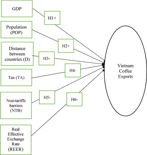
The hypotheses posed for the research model are as follows:

Hypothesis H1: As GDP of both countries increases, Vietnam’s coffee exports increase.

Hypothesis H2: As the population of both countries increases, Vietnam’s coffee exports will increase

Hypothesis H3: When the distance between the two countries is further and further away, Vietnam’s coffee exports will decrease

Hypothesis H4: The higher the tax rate between the two countries, the lower the coffee exports of Vietnam

Hypothesis H5: As the number of non-tariff barriers increases, Vietnam’s coffee exports decrease

Hypothesis H6: The higher the real effective exchange rate, the lower the coffee exports of Vietnam

That is, GDP and population factors have a positive influence on Vietnam’s coffee exports, while factors such as the distance between the two countries, tax rates, the number of non-tariff barriers, the exchange rate have a positive effect on coffee exports.

4.2. Empirical analysis model and data

This study analyzes the impact of factors such as economic size, population, tariffs, and exchange rates on Vietnam coffee exports with its 20 major partners from 2005 to 2019. Therefore, the study focuses on analyzing the factors affecting coffee export by gravity model. The basic gravity model hypothesis is as follows: (6) $$\mathbf{\text{ln}}\left({\mathit{Y}}_{\mathit{\text{odt}}}\right)={\mathit{c}}_0+{\mathit{\beta }}_1\mathbf{l}\mathbf{n}\left({\mathit{\text{GDP}}}_{\mathit{\text{ot}}}\right)+{\mathit{\beta }}_2\mathbf{l}\mathbf{n}\left({\mathit{\text{GDP}}}_{\mathit{\text{dt}}}\right)+{\mathit{\beta }}_3\mathbf{l}\mathbf{n}\left({\mathit{\text{POP}}}_{\mathit{\text{ot}}}\right)+{\mathit{\beta }}_4\mathbf{l}\mathbf{n}\left({\mathit{\text{POP}}}_{\mathit{\text{dt}}}\right)+{\mathit{\beta }}_5\mathbf{l}\mathbf{n}\left({\mathit{D}}_{\mathit{\text{ot}}}\right)+{\mathit{\beta }}_6\mathbf{l}\mathbf{n}\left(\mathit{\text{PRO}}\right.\mathrm{ }\left.{\mathit{D}}_{\mathit{\text{ot}}}\right)+{\mathit{\beta }}_7\mathbf{l}\mathbf{n}\left(\mathit{\text{PRO}}\right.\mathrm{ }\left.{\mathit{D}}_{\mathit{\text{dt}}}\right)+{\mathit{\beta }}_8\mathbf{l}\mathbf{n}\left({\mathit{\text{TA}}}_{\mathit{\text{ot}}}\right)+{\mathit{\beta }}_9\mathbf{l}\mathbf{n}\left({\mathit{\text{TA}}}_{\mathit{\text{dt}}}\right)+{\mathit{\beta }}_{10}\mathbf{l}\mathbf{n}\left({\mathit{\text{NTB}}}_{\mathit{\text{ot}}}\right)+{\mathit{\beta }}_{11}\mathbf{l}\mathbf{n}\left({\mathit{\text{NTB}}}_{\mathit{\text{dt}}}\right)+{\mathit{\beta }}_{12}\mathbf{l}\mathbf{n}\left({\mathit{\text{REER}}}_{\mathit{\text{ot}}}\right)+{\mathit{\beta }}_{13}\mathbf{l}\mathbf{n}\left({\mathit{\text{REER}}}_{\mathit{\text{dt}}}\right)+{\mathit{\delta }}_1{\mathit{\text{OECD}}}_{\mathit{\text{od}}}+{\mathit{\delta }}_2{\mathit{\text{APEC}}}_{\mathit{\text{od}}}+{\mathit{\delta }}_3{\mathit{\text{FTA}}}_{\mathit{\text{odt}}}+{\mathit{ϵ}}_{\mathit{\text{odt}}}$$(6)

In which: $c_0$: Constants; $Y_{\mathit{\text{odt}}}$: Output of exported coffee between country $o$ and country $d$ in year $t$; ${\mathit{\text{GDP}}}_{\mathit{\text{ot}}},{\mathit{\text{GDP}}}_{\mathit{\text{dt}}}$: Gross domestic product of country $o$ and country $d$ in year $t$; ${\mathit{\text{POP}}}_{\mathit{\text{ot}}},{\mathit{\text{POP}}}_{\mathit{\text{dt}}}$: Population of country $o$ and country $d$ in year $t$; $D_{\mathit{\text{ot}}}$: Distance between country $o$ and country $d$ in year $t$$\prod \_\mathit{\text{ot}},\prod \_\mathit{\text{dt}}$: The output of coffee exports from country $o$ and country $d$ in year $t$; ${\mathit{\text{TA}}}_{\mathit{\text{ot}}}$, ${\mathit{\text{TA}}}_{\mathit{\text{dt}}}$: Tax rates for coffee products of country $o$ and country $d$ in year $t$; ${\mathit{\text{NTB}}}_{\mathit{\text{ot}}},{\mathit{\text{NTB}}}_{\mathit{\text{dt}}}$: Number of non-tariff barriers to coffee in country $o$ and country $d$ in year $t$; ${\mathit{\text{REER}}}_{\mathit{\text{ot}}},{\mathit{\text{REER}}}_{\mathit{\text{dt}}}$: real effective exchange rate in country $o$ and country $d$ in year $t$; ${\mathit{\text{OECD}}}_{\mathit{\text{od}}}$: Dummy variable representing the presence or absence of OECD in country $o$ and country $d$; ${\mathit{\text{APE}}}_{\mathit{\text{od}}}$: Dummy variable representing the presence or absence of APEC in country $o$ and country $d$; ${\mathit{\text{FTA}}}_{\mathit{\text{odt}}}$: Dummy variable representing the signing of a free trade agreement between country $o$ and country $d$; $\beta ,\delta$: Coefficient of each explanatory variable; ${ϵ}_{\mathit{\text{odt}}}$: Error term.

The gravity model of this study employed panel data, time series and cross-sectional data to analyze the determinants influencing coffee exports. The 20 target countries⁴, as the main coffee export markets of Vietnam, were analyzed based on statistics on import and export of World Trade Organization (WTO). However, one of the target countries, Laos, was rejected due to insufficient data from UN Comtrade, therefore, panel gravity modeling analysis was performed for 19 countries.

Gross domestic product (GDP) and population data are independent variables. These data are taken from World Databank and World Development Indicator, which include the gross domestic product (GDP) and the population of the country of origin and the country of destination.

Dependent variable of the gravity model, based on data from UN Comtrade Database, International Trade on the coffee export value of each country in the form of bilateral trade.

The purpose of this study is to analyze the determinants influencing coffee exports. The dependent variable is total exports of coffee products. For example, the distance between two countries is an important variable in gravity models which often is analyzed by using straight-line geographic distances. However, in this study the difference between the ports of the trading countries was used as a distance variable. The tax rates for different coffee products in each country were classified and formulated according to the HS code, and then was applied as the real effective exchange rate index as well as consumer price index to calculate the experiment. In this study, the real effective exchange rate is used to reflect changes in relative prices for trading partners. It is calculated by adjusting the nominal exchange rate to weighted average relative prices with trading partners. The real effective exchange rate is calculated relative to the real exchange rate when two or more trading partners represent the real purchasing power of the local currency. Tran (2013) reported that if the real effective exchange rate at the time of comparison increases by 10% from the basis point, this means that the country’s currency has depreciated significantly by 10% from a basis point, it also indicates that the competitiveness is increasing a lot. This real effective exchange rate represents a country’s international competitiveness with respect to its trading partners. Analysis through the real effective exchange rate is a useful indicator for analyzing the price competitiveness of exported products and measuring changes in the value of Vietnamese Dong in response to changes in the relative price level for major trading partners.

In general, the gravity model is a model that analyzes the scale of bilateral trade using geographical and economic factors such as distance between countries, population, economies of scale and other influencing factors. In the case of tariffs, the tax rate is inversely proportional to the volume of trade between the two countries, indicating that the higher the tax rate, the higher the cost of trade that affects the volume of trade (Dang et al., 2020). The signing of regional trade agreements or free trade agreements has affected the amount of trade between the two countries, if this coefficient is positive, the free trade agreement (FTA) shows an effect of increasing trade.

4.3. Test for spatial autocorrelation

The LM (Lagrange Multiplier) test is performed on the spatial lag variables and the spatial errors to test whether there is spatial dependence among trading partners in coffee exports. The spatial weighting matrix is used to test the hypothesis of the inverse distance matrix and the three trade flow criteria (origin, origin and destination) to form a more weighted inverse distance squared matrix. Spatial autocorrelation test results are shown in Table 2, below:

Table 2. Spatial autocorrelation test result.

	Inverse distance matrix $\left(\frac{1}{d_{\mathit{\text{ij}}}}\right)$			Inverse distance square matrix $\left(\frac{1}{d_{\mathit{\text{ij}}}^2}\right)$
	${\mathit{W}}_{\mathit{o}}$	${\mathit{W}}_{\mathit{d}}$	${\mathit{W}}_{\mathit{w}}$	${\mathit{W}}_{\mathit{o}}$	${\mathit{W}}_{\mathit{d}}$	${\mathit{W}}_{\mathit{w}}$
LM-lag test	78.0 (0.00)	92.7 (0.00)	43.8 (0.00)	78.0 (0.00)	82.5 (0.00)	36.1 (0.00)
LM-error test	145.6 (0.00)	125.3 (0.00)	133.8 (0.00)	145.6 (0.00)	98.8 (0.00)	112.5 (0.00)

According to Table 2, the Spatial LM lag test index is ${(\chi }^2\left(1\right))$ is 36.1 ∼ 82.5 and the Spatial LM error test statistic is 98.8 ∼ 145.6. The results showed that spatial autocorrelation exists for variables and errors in all spatially weighted matrices. In this way, when spatial delay and error variables coexist with spatial magnetic field measurements, the general spatial gravity model could be the best fit.

4.4. Hypothesis test and panel data model selection

The statistical results showed that the F-test is 55.24. This indicates that there is an autocorrelation by rejecting the null hypothesis at the 1% significance level. The reason for the existence of autocorrelation is that the effect of an unexpected shock to exports persists for a certain period. The dependent variable is not only affected by the current effect, but also by the previous effects. In this case, autocorrelation already exists. Since there is autocorrelation in the dependent variable, it is more likely to lead to biased estimates with only static analysis. Therefore, dynamic analysis can be performed by adding lag-dependent variables to the analytical model.

The panel data model can be divided into fixed effects model and random effect model according to the specific effects of panel data. The hypothesis testing statistics and the results of the panel data model selection test are presented in Table 3, below:

Table 3. Hypothesis testing and panel data model selection.

	Fixed effects model	Random effects model	Hausman test	Autocorrelation test over time
	F test	χ^2 test	χ^2 test	F test
Static analysis	25.14* (0.00)	14067.32* (0.00)	262.63* (0.00)	55.24* (0.00)
Dynamic analysis	73.48* (0.00)	0.00 (1.00)	–

Note: * mean at 5%.

Analytical modeling is a method of analysis, comparative estimation is performed through static estimation analysis and dynamic estimation analysis. The panel data analysis model is built according to the tariff, exchange rate variables, tariff schedules, and the total tax rates of coffee products. For the exchange rate, a real effective exchange rate variable is adjusted for fluctuations in prices, the consumer price index and averaged for the share of coffee exports and real effective exchange rate index obtained by real Gross Domestic Product (GDP). According to the results of the fixed effect test through the F-test, the fixed effect is significant. In the results of Hausman test with effective comparison of the estimates of the fixed effects model and the estimates of the random effects model, it is showed that the fixed effect model is more suitable than the random effect model.

4.5. Empirical analytical model

Based on the results of hypothesis testing performed above, the General spatial fixed effect panel gravity model is the most suitable for the final empirical analysis in this study as follows: $$\mathbf{\text{ln}}\left({\mathit{Y}}_{\mathit{\text{odt}}}\right)={\mathit{c}}_0+{{\mathit{\rho }}_{\mathit{\eta }\mathit{\tau }}{\mathit{W}}_{\mathit{\eta }\mathit{\tau }}\mathbf{l}\mathbf{n}\left({\mathit{Y}}_{\mathit{\text{odt}}-1}\right)+\mathit{\beta }}_1\mathbf{l}\mathbf{n}\left({\mathit{\text{GDP}}}_{\mathit{\text{ot}}}\right)+{\mathit{\beta }}_2\mathbf{l}\mathbf{n}\left({\mathit{\text{GDP}}}_{\mathit{\text{dt}}}\right)+{\mathit{\beta }}_3\mathbf{l}\mathbf{n}\left({\mathit{\text{POP}}}_{\mathit{\text{ot}}}\right)+{\mathit{\beta }}_4\mathbf{l}\mathbf{n}\left({\mathit{\text{POP}}}_{\mathit{\text{dt}}}\right)+{\mathit{\beta }}_5\mathbf{l}\mathbf{n}\left({\mathit{D}}_{\mathit{\text{odt}}}\right)+{\mathit{\beta }}_6\mathbf{l}\mathbf{n}\left(\mathit{\text{PRO}}\right.\mathrm{ }\left.{\mathit{D}}_{\mathit{\text{ot}}}\right)+{\mathit{\beta }}_7\mathbf{l}\mathbf{n}\left(\mathit{\text{PRO}}\right.\mathrm{ }\left.{\mathit{D}}_{\mathit{\text{dt}}}\right)+{\mathit{\beta }}_8\mathbf{l}\mathbf{n}\left({\mathit{\text{TA}}}_{\mathit{\text{ot}}}\right)+{\mathit{\beta }}_9\mathbf{l}\mathbf{n}\left({\mathit{\text{TA}}}_{\mathit{\text{dt}}}\right)+{\mathit{\beta }}_{10}\mathbf{l}\mathbf{n}\left({\mathit{\text{NTB}}}_{\mathit{\text{ot}}}\right)+{\mathit{\beta }}_{11}\mathbf{l}\mathbf{n}\left({\mathit{\text{NTB}}}_{\mathit{\text{dt}}}\right)+{\mathit{\beta }}_{12}\mathbf{l}\mathbf{n}\left({\mathit{\text{REER}}}_{\mathit{\text{ot}}}\right)+{\mathit{\beta }}_{13}\mathbf{l}\mathbf{n}\left({\mathit{\text{REER}}}_{\mathit{\text{dt}}}\right)+{\mathit{\delta }}_1{\mathit{\text{OECD}}}_{\mathit{\text{od}}}+{\mathit{\delta }}_2{\mathit{\text{APEC}}}_{\mathit{\text{od}}}+{\mathit{\delta }}_3{\mathit{\text{FTA}}}_{\mathit{\text{odt}}}+{\mathit{ϵ}}_{\mathit{\text{odt}}}$$ (7) $$({\mathit{ϵ}}_{\mathit{\text{odt}}}={\mathit{\lambda }}_{\mathit{\eta }\mathit{\tau }}{\mathit{W}}_{\mathit{\eta }\mathit{\tau }}{\mathit{ϵ}}_{\mathit{\text{odt}}}+{\mathit{u}}_{\mathit{\text{odt}}})$$(7)

In model (7) the coefficients of the lag dependent variable, other variables and coefficients are the same as in model (6). The coefficient of continuous variation of the general linear logarithmic model of gravity means elasticity. However, in the spatial gravity model, the spatially dependent variable $W\mathrm{\text{ln}}\left(Y\right)$ exists, so the elasticity is calculated as follows: (8) $$\frac{\partial \mathbf{\text{ln}}\left(\mathit{Y}\right)}{\partial \mathbf{\text{ln}}\left(\mathit{X}\right)}=\frac{1}{{\mathit{n}}^2}{\mathit{\iota }}_{{\mathit{n}}^2}^{,}\left[\mathit{\theta }{\left(\mathit{I}-{\mathit{\rho }}_{\mathit{\eta }\mathit{\tau }}{\mathit{W}}_{\mathit{\eta }\mathit{\tau }}\right)}^{-1}\right]{\mathit{\iota }}_{{\mathit{n}}^2}=\frac{1}{{\mathit{n}}^2}\left[\sum _{\mathit{i}=1}^{{\mathit{n}}^2}\sum _{\mathit{j}=1}^{{\mathit{n}}^2}{\mathit{\upsilon }}_{\mathit{\text{ij}}}\mathit{\theta }\right]$$(8) $n$ is the number of countries; $X$ is vectors of continuous variables; $\theta$ is the number of continuous variables.

In the spatial econometric model, the model (8) is called Average total effect. (9) $$\frac{1}{{\mathit{n}}^2}\mathit{t}\mathit{r}\left[\mathit{\theta }{\left(\mathit{I}-{\mathit{\rho }}_{\mathit{\eta }\mathit{\tau }}{\mathit{W}}_{\mathit{\eta }\mathit{\tau }}\right)}^{-1}\right]=\frac{1}{{\mathit{n}}^2}\left[\sum _{\mathit{i}=1}^{{\mathit{n}}^2}{\mathit{\upsilon }}_{\mathit{\text{ij}}}\mathit{\theta }\right]$$(9)

LeSage and Pace (2008) suggested that this can be broken down into Average direct effect, Average indirect effect, and average total effect. The average indirect effect is the total effect minus the direct effect. These are the average effects on the export value of the i-th trader when X increases by 1%.

4.6. Experimental analysis results

The estimated results using the experimental model are presented in Table 4. The estimated results of the panel data gravity model that do not consider the existing spatial dependence are presented in Model (1). For the estimated results of the fixed effects generalized spatial gravity model, the panel data (inverse distance matrix, inverse distance squared matrix) has a larger spatial weight.

Table 4. Estimated results of experimental models.

Variables	Model 1	Model 2 ${\mathit{W}}_{\mathit{d}}$	Model 3 ${\mathit{W}}_{\mathit{o}}$	Model 4 ${\mathit{W}}_{\mathit{w}}$	Model 5 ${\mathit{W}}_{\mathit{d}}$	Model 6 ${\mathit{W}}_{\mathit{o}}$	Model 7 ${\mathit{W}}_{\mathit{w}}$
		Inverse distance matrix (1/${\mathit{d}}_{\mathit{\text{ij}}}$)			Inverse distance square matrix (1/${\mathit{d}}_{\mathit{\text{ij}}}^2$)
Lag dependent variable	0.391* (−0.012)	0.265* (0.010)	0.228* (0.010)	0.302* (0.010)	0.223* (0.010)	0.208* (0.010)	0.285* (0.011)
${\mathit{\text{GDP}}}_o$	0.621* (−0.211)	0.818* (0.224)	0.165 (0.425)	1.169* (0.240)	0.621* (0.218)	0.134 (0.340)	1.133* (0.223)
${\mathit{\text{GDP}}}_d$	0.643* (−0.201)	0.729* (0.254)	0.934* (0.203)	1.027* (0.205)	0.716* (0.243)	0.820* (0.202)	0.867* (0.207)
${\mathit{\text{POP}}}_o$	−4868* (−1.257)	−5.010* (1.304)	−9.426* (2.622)	−2.873* (1.335)	−7.012* (1.268)	−8.381* (1.859)	−5.846* (1.502)
${\mathit{\text{POP}}}_d$	5.210* (−1.254)	9.231* (1.854)	8.351* (1.209)	9.215* (1.348)	7.150* (1.508)	7.458* (1.214)	8.263* (1.303)
	−0.428* (−0.183)	−0.836* (0.300)	−0.524 (0.482)	−1584* (0.223)	0.547* (0.242)	−0.417 (0.268)	−1.55* (0.315)
${\mathit{\text{PROD}}}_o$	0.211 (−0.220)	0.368* (0.206)	0.813 (0.410)	0.148 (0.201)	0.619* (0.216)	0.846* (0.309)	0.379 (0.210)
${\mathit{\text{PROD}}}_d$	0.003 (−0.102)	−0.055* (0.101)	−0.072 (0.130)	−0.085 (0.080)	−0.015 (0.100)	−0.081 (0.121)	−0.048 (0.090)
${\mathit{\text{TA}}}_o$	0.324 (−0.401)	0.768* (0.344)	0.833 (0.905)	0.551 (0.364)	1.026* (0.401)	0.807 (0.615)	0.844* (0.401)
${\mathit{\text{TA}}}_d$	−2.024* (−0.416)	−2.468* (0.549)	−2.354* (0.312)	−2.507* (0.383)	−2.906* (0.505)	−2.670* (0.325)	−2.468* (0.384)
${\mathit{\text{SPS}}}_o$	−0.006 (−0.050)	0.026* (0.042)	−0.071 (0.101)	0.035 (0.043)	0.020 (0.046)	−0.061 (0.081)	0.041 (0.048)
${\mathit{\text{SPS}}}_d$	0.016 (−0.043)	−0.038* (0.071)	−0.009 (0.044)	−0.006 (0.045)	−0.035 (0.060)	−0.019 (0.042)	−0.021 (0.044)
${\mathit{\text{TBT}}}_o$	0.186* (−0.071)	0.061* (0.073)	0.073 (0.170)	0.083 (0.080)	0.062 (0.081)	0.076 (0.128)	0.103 (0.088)
${\mathit{\text{TBT}}}_d$	−0.134* (−0.068)	−0.403* (0.015)	−0.325* (0.072)	−0.315* (0.081)	−0.429* (0.091)	−0.369* (0.083)	−0.340* (0.082)
${\mathit{\text{REER}}}_o$	−1.142* (−0.286)	−1.465* (0.283)	−1.192* (0.540)	−1.600* (0.271)	−1.325* (0.283)	−1.108* (0.448)	−1.530* (0.290)
${\mathit{\text{REER}}}_d$	−0.148 (−0.210)	0.356* (0.255)	0.127 (0.231)	0.003 (0.240)	0.425 (0.250)	0.357 (0.242)	0.193 (0.236)
$\mathit{\text{OECD}}$	−0.169 (−0.266)	−0.04* (0.276)	−0.156 (0.310)	−0.186 (0.274)	0.048 (0.270)	−0.091 (0.296)	−0.126 (0.272)
$\mathit{\text{APEC}}$	−0.365 (−0.329)	0.091* (0.321)	0.305 (0.501)	0.076 (0.311)	0.025 (0.321)	0.281 (0.440)	0.014 (0.306)
$\mathit{\text{FTA}}$	0.120 (−0.156)	0.045* (0.151)	−0.206 (0.170)	−0.078 (0.173)	0.073 (0.172)	−0.132 (0.181)	0.021 (0.173)
$\rho$	−0.906* (0.102)	−0.539* (0.047)	−0.171* (0.051)	−0.912* (0.108)	−0.289* (0.034)	−0.088* (0.035)	−0.324* (0.041)
$\lambda$	0.871* (0.022)	0.550* (0.024)	0.589* (0.025)	0.817* (0.026)	0.341* (0.027)	0.408* (0.026)	0.625* (0.028)
$R^2$	0.021	0.068	0.032	0.115	0.035	0.034	0.080
LL (Log-Likelihood)		−12907	−12663	−12833	−12961	−12752	−12889

Note: * means at 5% level.

In Table 4, six models (Models 2 to 7) have been presented, combining inverse matrix, destination criteria $(W_d)$, origin criteria $(W_o)$ and origin – destination $(W_w)$. The results illustrate that the effect of distance, oil price, tax rate, non-tariff barriers and real effective exchange rate are the main variables of this study. Except for Model (6), the remaining models are found to affect trade flows between the two countries. Tax rates, non-tariff barriers, and real effective exchange rates all have significant effects in the six spatial gravity models and are analyzed as factors affecting exports. As tax rates, non-tariff barriers and the real effective exchange rate increase, the exports appear to fall. According to the model selection process in the spatial econometric model, the coefficients estimated due to the existence of the spatial difference dependent variable ($\mathit{\text{WY}}$) cannot exactly explain the elasticity.

Therefore, the sum of effects (elastic), direct effects and indirect effects use models (8) and (9). The results show that, among the seven models presented, the model 4 with the highest $R^2=1.15$ is selected to estimate the elasticity.

Therefore, the elasticity estimation results of Model 4 are as follows (Table 5).

Table 5. Elasticity analysis results (based on model 4).

Variables	Coefficient	Total impact	Direct impact	Indirect effects
Lag dependent variable	0.302* (0.010)	0.155* (0.010)	0.301* (0.010)	−0.142* (0.010)
${\mathit{\text{GDP}}}_o$	1.169* (0.240)	0.613* (0.132)	1.174* (0.240)	−0.563* (0.121)
${\mathit{\text{GDP}}}_d$	1.027* (0.205)	0.542* (0.106)	1.046* (0.194)	−0.501* (0.098)
POPo	−2.873* (1.335)	−1580* (0.703)	−3.028* (1.430)	1.421* (0.680)
${\mathit{\text{POP}}}_d$	9.215* (1.348)	4.832* (0.751)	9.340* (1.340)	−4.506* (0.710)
$D$	−1584* (0.223)	−0.845 (0.270)	−1.608* (0.482)	−0.703* (0.728)
${\mathit{\text{PROD}}}_o$	0.148 (0.201)	0.086 (0.112)	0.172 (0.217)	−0.084 (0.103)
${\mathit{\text{PROD}}}_d$	−0.085 (0.080)	−0.041 (0.050)	−0.085 (0.092)	0.048 (0.041)
${\mathit{\text{TA}}}_o$	0.551 (0.364)	0.287 (0.186)	0.556 (0.371)	−0.266 (0.180)
${\mathit{\text{TA}}}_d$	−2.507* (0.383)	−1,325 (0.224)	−2.550* (0.389)	1.230* (0.202)
${\mathit{\text{SPS}}}_o$	0.035 (0.043)	0.016 (0.024)	0.032 (0.043)	−0.014 (0.021)
${\mathit{\text{SPS}}}_d$	−0.006 (0.045)	−0.003 (0.028)	−0.068 (0.042)	0.002 (0.011)
${\mathit{\text{TBT}}}_o$	0.083 (0.080)	0.041 (0.045)	0.081 (0.092)	−0.044 (0.041)
${\mathit{\text{TBT}}}_d$	−0.315* (0.081)	−0,173* (0.040)	−0.322* (0.071)	0.151* (0.036)
${\mathit{\text{REER}}}_o$	−1.600* (0.271)	−0,845 (0.150)	−1618* (0.264)	0.745* (0.142)
${\mathit{\text{REER}}}_d$	0.003 (0.240)	−0.002 (0.115)	−0.005 (0.271)	0.093 (0.132)
$\mathit{\text{ECD}}$	−0.186 (0.274)	−0.104 (0.142)	0.194 (0.272)	0.090 (0.132)
$\mathit{\text{APEC}}$	0.076 (0.311)	0.051 (0.168)	0.102 (0.328)	−0.050 (0.152)
$\mathit{\text{FTA}}$	−0.078 (0.173)	−0.040 (0.086)	−0.081 (0.172)	0.039 (0.085)
$\rho$	−0.912* (0.108)
$\lambda$	0.817* (0.026)
LL (Log-Likelihood)	−12833

Note: * means at 5% level.

The elasticity to the tax rate is −1.325, the elasticity for non-tariff barriers is −0.173 and the elasticity for the real effective exchange rate is −0.846, different from the elasticity of the panel data gravity model is due to the direct effect of the reduction in exports due to increased tariffs, increased non-tariff barriers and an increase in the real effective exchange rate in origin-destination trade of −1.324; −0.173, and −0.846, but due to the indirect effect of countries adjacent to the origin and destination, the elasticity is different. In other words, it is analyzed that the elastic number is different by adding together the direct effects of changes in exports with changes in the influence factor in point of origin-destination trade, plus the indirect effects of countries contiguous to the point of origin destination. This means that the bias of the estimator is reduced when considering the spatial dependence in the estimation results of the spatial gravity model. considering the $\rho$ coefficient of the spatial difference dependent variable (WY) has a negative sign (−), shows signs of indirect effects and direct effects are reversed, revealing that the origin-destination adjacency matrix with an average increase in the exports of neighboring countries will decrease the exports of the trading partners. Therefore, the increase in exports of coffee products between specific trading partners has a negative spillover effect on the exports of neighboring countries. Thus, coffee exports neighboring countries are competing with each other by producing and exporting similar commodities.

5. Discussion and conclusion

In this study, factors affecting Vietnam coffee exports are analyzed by means of spatial gravity model through panel data to consider spatial dependence in gravity model. The main analysis results are as follows.

First, an increase in GDP and population can positively affect exports. This is in consistent with existing gravity model theory and is considered to reflect reality well. This result is also consistent with hypotheses H1 and H2, meaning that when the GDP of both countries increases, Vietnam’s coffee exports increase. And as the populations of both countries increase, Vietnam’s coffee exports increase.

Second, the distance between two countries is calculated through an elasticity to the oil price gap of -0.845 indicating an increased gap will cause exports to fall. This is consistent with hypothesis H3, meaning that as the distance between the two countries becomes bigger, Vietnam’s coffee exports will decrease.

Third, the higher the tax rates, non-tariff barriers, and the real effective exchange rate, the lower exports are, which are factors that negatively affect exports. This result is consistent with hypotheses H4, H5 and H6, meaning that the higher the tax rate between the two countries, the lower Vietnam’s coffee exports. When the number of non-tariff barriers is greater, Vietnam’s coffee exports decrease, and when the real effective exchange rate is higher, Vietnam’s coffee exports decrease.

Thus, it can be observed that the research findings support the theory that has been put forward, and this finding is remarkably comparable to those of Beenstock and Felsenstein (2013).

The recent changing trend of the trade environment is that the tax rate is decreasing due to the increase in the number of trade agreements such as FTAs between trading partners, which is expected to have a positive impact on coffee exports. On the other hand, due to the exchange rate policy, the economic situation of each country is different, and the policies to improve competitiveness cause the exchange rate to rise, negatively affecting exports. In addition, non-tariff barriers, unlike tariffs, which are difficult to understand and not quantified, operate individually in each country, making it difficult to find solutions to improve. Therefore, if it is possible to develop countermeasures to the factors that negatively affect exports and improve the factors that positively affect exports to help Vietnam establish a more developed coffee export market.

Fourth, in the estimation results of the spatial gravity model, the signs of indirect effects and direct effects are different, the results of the analysis have shown that export flows between specific trading partners can create a ripple effect that has a negative impact on exports between neighboring countries. In addition, Vietnam can apply high technology to coffee production to help increase export value, make the most of natural resources, labor force, production equipment, to improve efficiency and quality of exported coffee products.

However, this study is limited in that it only examines the variables influencing the export of coffee products from Vietnam to the 20 largest export markets as of 2019. In addition, because the dependent variable was the total export value of coffee products, it was not possible to perform a breakdown by coffee item. Due to the lack of randomness in the use of the matrix to identify the spatial dependence, the study can also be arbitrarily studied. It is possible to examine and test the model using various matrices while accounting for geographical dependence in later research. Moreover, a more comprehensive examination of factors that influence Vietnam’s coffee exports and its policy implications can be conducted.

Disclosure statement

No potential conflict of interest was reported by the author(s).

Additional information

Notes on contributors

Thuy Dung Vo

Thuy Dung Vo is a lecturer at Van Lang University, Vietnam. She is currently working as a doctoral student at East China Normal University, Shanghai, China. Her interests are international economics and business.

Laike Yang

Laike Yang is a professor, and Director of the International Trade Department of the East China Normal University, Shanghai, China. He got PhD at Xiamen University in China. His interests are International Trade and the Environment, Upgrading of the global value chain and trade structure, Regional economic integration, production segmentation and technological progress.

Manh Dung Tran

Manh Dung Tran is an Associate Professor, and senior lecturer at the National Economics University, Vietnam. He is now a Deputy Editor-in-Chief of the Journal of Economics and Development. He got PhD at Macquarie University in Australia. His interests are international economics and business, finance, and management.

Notes

1 Spatial Lag refers to the case where the dependent variables of country i are affected simultaneously by the explanatory variables of country i and country j. Therefore, the dependent variables and the error are also correlated with each other.

2 Spatial Error is a case where spatial units are linked between errors with different spatial units. Thus, in this case, the basic statistical assumption is violated and becomes less efficient when the estimate does not consider spatial effects.

3 Model (3), $W_{o}Y$ stands for the typical invisible flow between the neighboring nations of the origin (o) and the destination (d). To put it another way, imagine that nations a, b, and c are close to the beginning location and that countries k, l, and m are close to the destination. The average trade flow between origin (o) and destination (d) in nations a, b, and c is $W_{o}Y$. $W_{d}Y$ denotes the average amount of trade flowing from the origin to the nearby countries (k, l, and m). The average of trade flows from countries a, b, and c near the origin to countries k, l, and m near the destination is represented by the term W_w. The unbiasedness of the estimated result serves as a measure of the estimate’s accuracy. If an estimator uses or takes advantage of all the data-related information and model assumptions in its computation, it is said to be efficient. When evaluating the spatial dependency between mistakes in the spatial gravity model, the combination of spatial error variables (Wu) is important, and its significance is comparable to that of the difference dependent variable of time.

4 20 countries including Germany, USA, Italy, Spain, Japan, Philippines, Russia, Belgium, Algeria, Thailand, Israel, Indonesia, China, South Africa, Cambodia, Chile, Singapore, Myanmar, Hungary, Poland, Laos.

References

- Anselin, L. (1988). Spatial econometrics: Methods and models (Vol. 4). Springer Science & Business Media. https://link.springer.com/book/10 .1007/978-94-015-7799-1; https://scholar.google.com/scholar_lookup?hl=en&publication_year=1988&author=L.+Anselin&title=Spatial+econometrics+methods+and+models
- Beenstock, M., & Felsenstein, D. (2013). Modeling ENP-EU migration in a spatial gravity.
- Bui, T. T. M. (2020). LASSO estimation method: Mathematical foundations and applications. Journal of Asian Business and Economic Studies, 31, 1–16.
- Dang, T. T., Zhang, C. H., Nguyen, T. H., & Nguyen, N. T. (2020). Assessing the influence of exchange rate on agricultural commodity export price: evidence from Vietnamese coffee. Journal of Economics and Development, 22(2), 297–309. https://doi.org/10.1108/JED-02-2020-0014
- Do, T. H. N. (2019). Analysis of factors affecting Vietnam’s agricultural exports to the EU market. TNU Journal of Science and Technology, 196(03), 35–44.
- Evenett, S. J., & Keller, W. (2002). On theories explaining the success of the gravity equation. Journal of Political Economy, 110(2), 281–316. https://doi.org/10.1086/338746
- Gautschi, D. A. (1981). Specification of patronage models for retail center choice. Journal of Marketing Research, 18(2), 162–174. https://doi.org/10.2307/3150951
- Griffith, D. (2007). Spatial structure and spatial interaction: 25 years later. Review of Regional Studies, 37(1), 28–38. https://doi.org/10.52324/001c.8286
- Leibenstein, H., & Tinbergen, J. (1962). Shaping the world economy: Suggestions for an international economic policy. Economic Journal, 76(301), 92–95. https://doi.org/10.2307/2229041
- LeSage, J. (1999). The theory and practice of spatial econometrics. University of Toledo. https://d1wqtxts1xzle7.cloudfront.net/55768690/sbook-libre.pdf?1518297040=&response-contentdisposition=inline%3B+filename%3DThe_theory_and_practice_of_spatial_econo.pdf&Expires=1713268784&Signature=R3DvXxR79IhopfIdFw4bGRME66jZwWiIhIWY8Ar-vw9FksMj3GgBrr∼u-U2zt0HyR7yYsIHRQ∼d97UsU3iRL4L3vzKGEmzSJ6P5aQ2pCZV41RpmR7kBu5l9oecKhllkWXiOoYP4RYLAwxDQT7zjQjLQH3rqXtk03lOK678uXl1xJRgcnosvzoZWAd4wIWIpKlCgmCWnRczjLl6yW5wtu∼zKnoE3L6x0NDaMgdAXCdYHc6oVrJYcPaFon0pXQFHvkaZYpspVNZ4J3me854H∼jthr62RNg00HTsNnha∼ptaKsy∼∼hetR0K3IQP5jIdlTbmOWp∼Rxlo7jdDhwj42kQ__&Key-Pair-Id=AP KAJLOHF5GGSLRBV4ZA
- LeSage, J., & Pace, R. K. (2008). Spatial econometric modeling of origin-destination flows. Journal of Regional Science, 48(5), 941–967. https://doi.org/10.1111/j.1467-9787.2008.00573.x
- LeSage, J., & Pace, R. K. (2009). Introduction to spatial econometrics. Chapman.
- Nguyen, T. S. (2012). US-ASEAN Relations, 2001-2020. Hanoi Publishing House, Ha Noi.
- Nguyen, T. T. H. (2021). Promoting coffee exports to the EU market in the context of EVFTA implementation. Journal of Industry and Trade, 6, 83-87.
- Nguyen, V. S. (2020). Spatial regression application in export research in Vietnam: A provincial/city level approach. Science and Technology Development Journey – Economic – Law and Management, 3, 269–282.
- Rendleman, C. M., & Vasinvarthana, Y. (2013). Is the bioterrorism act a barrier to developing country seafood exporters. Social Science Research Network.
- Pham, N. M., Nguyen, T. N., &Le, H. K. (2018). Impacts of New Generation of Free Trade Agreements (FTAs) on the Development of Export - Import Markets of Members—Vietnam Case Study. Вьетнамские исследования, 2(3), 18–31. https://cyberleninka.ru/article/n/impacts-of-newgeneration-of-free-trade-agreements-ftas-on-the-development-of-export-import-markets-of-membersvietnam-case-study/viewer