Energy-Dependent, Self-Adaptive Mesh h(p)-Refinement of an Interior-Penalty Scheme for a Discontinuous Galerkin Isogeometric Analysis Spatial Discretization of the Multi-Group Neutron Diffusion Equation with Dual-Weighted Residual Error Measures

Abstract

Energy-dependent self-adaptive mesh refinement algorithms are developed for a symmetric interior-penalty scheme for a discontinuous Galerkin spatial discretization of the multi-group neutron diffusion equation using NURBS-based isogeometric analysis (IGA). The spatially self-adaptive algorithms employ both mesh (h) and polynomial degree (p) refinement. The discretized system becomes increasingly ill-conditioned for increasingly large penalty parameters; and there is no gain in accuracy for over penalization. Therefore, optimized penalty parameters are rigorously calculated, for general element types, from a coercivity analysis of the bilinear form. Local mesh refinement allows for a better allocation of computational resources; and thus, more accuracy per degree of freedom. Two a posteriori interpolation-based error measures are proposed. The first heuristically minimizes local contributions to the discretization error, which becomes competitive for global quantities of interest (QoIs). However, for localized QoIs, over energy-dependent meshes, certain multi-group components may become under-resolved. The second employs duality arguments to minimize important error contributions, which consistently and reliably reduces the error in the QoI.

Keywords:

• Multi-group neutron diffusion equation
• interior-penalty scheme
• discontinuous Galerkin
• isogeometric analysis
• energy-dependent self-adaptive mesh h(p)-refinement
• dual-weighted residual error measures

1. Introduction

The steady-state neutron diffusion equation (NDE) is an elliptic partial-integro-differential equation (PIDE); it is a function of spatial position (x, y, z); and energy (E). It is derived from the linearized form of the non-linear Boltzmann transport equation, the neutron transport equation (NTE), which describes the non-equilibrium average statistical behavior of gas atoms, or molecules (Boltzmann 1872). The NDE serves as a reasonable lower-order approximation to the NTE for the migration of neutrons in weakly-absorbing media, several mean-free paths (MFPs) away from isolated sources, external boundaries and heterogeneous-material interfaces (Hébert 2020).

Employing the multi-group approximation, the energy-dependent NDE can be reduced to a system of weakly-coupled partial differential equations (PDEs), which can then be spatially discretized. Wilson et al. present a thorough discussion of the finite element method (FEM) and FEM-based adaptive mesh refinement-h(p) (AMR-h(p)) techniques, including the use of energy-dependent meshes and different interpolation-based error measures; specifically, energy-driven (NRG) and dual-weighted residual (DWR) ones (Wilson, Eaton, and Kópházi 2024). They also provide the motivation for using isogeometric analysis (IGA) methods as high-fidelity spatial discretizations schemes for nuclear reactor physics problems (Wilson, Eaton, and Kópházi 2024). For brevity, these discussions are not repeated here.

Local-refinement strategies inevitably yield non-conforming, or hanging-node, meshes, whereby the patches may not be mathematically connected in a parametric sense. Although this does not pose any issue for computer-aided geometric design (CAGD), it does present one for the analysis of the governing equations posed over NURBS-based computational meshes. The NURBS patches must be coupled explicitly in order to produce a well-posed and solvable system of linear algebraic equations. There are a number of approaches to develop non-conforming spatial discretizations of elliptic PIDEs.

The work presented in this paper builds upon that of Wilson et al. (Wilson et al. 2018). They employed a symmetric interior penalty (SIP) scheme for a discontinuous Galerkin (DG) IGA spatial discretization of the multi-group NDE. Continuity in the numerical solution is weakly enforced between adjacent elements by calculating optimized penalty parameters, for general element types, from a rigorous coercivity analysis of the bilinear form (Owens, Kópházi, and Eaton 2017). Admittedly, when compared to a continuous Bubnov-Galerkin discretization over the same mesh, such a discontinuous spatial discretization requires at least double the DoFs.

Nitsche introduced penalty schemes to enforce weakly Dirichlet boundary conditions (BCs) by appending penalty terms to the bilinear form (Nitsche 1971). This penalization was then applied to the interior of the finite element mesh by Wheeler and by Percell and Wheeler as a means of weakly enforcing continuity across element interfaces (Wheeler 1978; Percell and Wheeler 1978). Interior penalty (IP-)DG-FEM were also developed independently by Arnold for general non-linear second-order elliptic and parabolic problems (Arnold 1982). More recently, IP schemes have been applied to IGA discretizations of elliptic systems (Brunero 2012; Wilson et al. 2018).

In the non-conforming and discontinuous setting, the variational boundary value problem (VBVP) is formulated locally over a given element and a projection of the residuals is made to be negligibly small across its boundaries (Rivière 2008). IP-DG methods are often compared to stabilized mixed FEM for second-order differential equations, since residual-based penalty terms are introduced to stabilize the discrete problem (Li 2006). There exist myriad IP schemes, each employing its own combination of penalty terms. Typically, the penalty terms take the form of weighted $L_2$-inner products of jumps in the trial and test functions at element interfaces; and the coupling of control-variables exists only between direct neighbors that share an interface (Arnold et al. 2002; Brezzi et al. 2006). From a practical point of view, the inevitable costs incurred in implementing an IP-DG scheme may be offset by its compact discretization stencil; and the flexibility offered in terms of mesh refinement (Di Pietro and Ern 2012). The choice of penalty parameters is crucial to the effectiveness of the numerical method. For arbitrarily large values, iterative smoothers can become slow to converge as the conditioning of the iteration matrix worsens (Castillo 2002). For values not large enough, the residual-based jumps across element boundaries may not be sufficiently penalized; in which case, coercivity of the bilinear can not be guaranteed. In the literature, penalty parameters are often assigned values based upon experience and numerical experiments (Alvarez et al. 2006). More often though, the penalty parameters are taken as some user-dependent sufficiently large constant that scales under refinement of the mesh (Douglas and Dupont 1976).

This paper considers both NRG-AMR-h(p) and DWR-AMR-h(p) strategies for a symmetric (S)IP-DG-IGA spatial discretization of the multi-group NDE. The work presented is based upon the author’s PhD thesis (Wilson 2021).

The basic notions of NURBS-based IGA and energy-dependent meshes are briefly introduced in Section 2; and the AMR-h(p) strategies and accompanying error measures are outlined in Section 3. The direct (primal) multi-group NDE, along with its physical adjoint (dual) equation, are presented in Section 4; and, as per a SIP-DG-IGA discretization, their weak-forms are derived in Section 5. Based upon the stiffness matrix approach by Owens et al. optimized penalty parameters are calculated from the trace inequality constants (TICs) for general element types, derived from a coercivity analysis of the bilinear form in Section 5.4 (Owens, Kópházi, and Eaton 2017). Finally, numerical results for reactor physics benchmark test cases are presented in Section 6 to verify the computational performance and accuracy of the AMR algorithms. The AMR-h(p) algorithms over energy-dependent meshes are compared to the uniform refinement of a single energy-independent mesh. Furthermore, the method of manufactured solutions (MMS) is used to investigate the numerical convergence of the AMR strategies compared to theoretical rates of convergence.

2. NURBS-based isogeometric analysis

The geometries of most engineering problems are produced from a basis of NURBS, or some other related spline-based description, used to generate complex surfaces bounding solid objects. The simplest description of the geometry is typically based upon a decomposition of the problem into its constituent material regions. Regardless, the physical domain is exactly represented by a tessellation of NURBS patches, the union of which forms the physical mesh, $\mathcal{T}(V).$ The geometrical mapping is a parametrization of $\overrightarrow{r}:\widehat{V}\to V,$ which takes a point in the parametric domain, ${\overrightarrow{r}}^{\text{−}1}\in \widehat{V}\subset {\mathbb{R}}^{\widehat{d}},$ where the NURBS basis is defined, and maps it to a point in Euclidean space, $\overrightarrow{r}\in V\subset {\mathbb{R}}^d,$ for $d,\widehat{d}=1,2\text{\hspace{0.5em}or\hspace{0.5em}}3.$ A NURBS basis function defined over the real physical space, $R(\overrightarrow{r}),$ is the composition of that function, $R({\overrightarrow{r}}^{\text{−}1}),$ with the inverse of the geometrical mapping; i.e., $R(\overrightarrow{r})=\{R({\overrightarrow{r}}^{\text{−}1})°{\overrightarrow{r}}^{\text{−}1}:\forall {\overrightarrow{r}}^{\text{−}1}\in \widehat{V}\}.$ The parametric domain is local to a given patch. Consequently, a NURBS basis function has finite local support on a single given patch, in both $\widehat{V}$ and V, as per the bijective mapping; i.e.,: (1) $$\text{supp}(R)=\{\overrightarrow{r}\in V_e:R(\overrightarrow{r})\ne 0,\forall {\overrightarrow{r}}^{\text{−}1}\in {\widehat{V}}_e\},\hspace{1em}\forall V_e\in \mathcal{T}(V).$$(1)

Multi-dimensional, $d>1,$ NURBS basis functions are constructed in a tensor-product fashion from univariate B-splines, which can be expressed via the Cox-de Boor recursion formula (Cox 1972; de Boor 1972). A description of the parametric domain, denoted by some parameter $0\le \xi \le 1$ in 1D, begins with an open knot-vector, ${\Xi }_{\xi },$ which is a set of non-decreasing coordinates: ${\Xi }_{\xi }={\left\{{\xi }_i\right\}}_{i=1}^{n+p+1},$ where ${\xi }_i$ are the knots; p is the polynomial degree of the basis; and n is the total number of basis functions that span ξ. Knots are points of reduced continuity that partition the parametric domain into knot-spans; the $i^{\mathit{\text{th}}}$ knot-span is defined by the half-closed interval $[{\xi }_i,{\xi }_{i+1}).$ A knot-value is said to have a multiplicity of $\dot{m}$ knots if $\dot{m}$ number of knots take on the same value. The continuity of the basis over any given knot-value is $C^{p-\dot{m}}.$ Within knot-spans of non-zero length, the basis is infinitely differentiable, $C^{\infty }$-continuous; i.e., for ${\xi }_i\ne {\xi }_{i+1}.$

Increasing the multiplicity of a knot to $\dot{m}=p$ renders the NURBS basis interpolatory at that given knot-value. Effectively, a new patch boundary is formed and $C^0$-continuity is naturally enforced across the new boundary; e.g. see Figure 3. For $\dot{m}=p+1,$ again, a new patch boundary is formed. However, now, the basis is discontinuous, or $C^{-1}$-continuous.

The NURBS basis functions inherit many of their properties from the B-splines; e.g. the convex hull property and the variation diminishing property (Piegl and Tiller 1997). The support of B-splines, ${\left\{N_i^p\right\}}_{i=1}^N,$ is compact and extends over $p+1$ knot-spans; i.e., for $i=1,\dots ,N:$ (2) $$\text{supp}(N_i^p)=\{\xi \in \widehat{V}\subset {\mathbb{R}}^1:N_i^p(\xi )\ne 0,\forall {\xi }_i\le \xi <{\xi }_{i+p+1}\}\text{;}$$(2) and $p+1$ functions always have support within any given knot-span.

Equation 3(3) $$R_{i,j}^{p,q}(\xi ,\eta )=\frac{N_i^p(\xi )M_j^q(\eta )W_{i,j}}{\sum _{i\prime =1}^N\sum _{j\prime =1}^M{N}_{i\prime }^p(\xi )M_{j\prime }^q(\eta )W_{i\prime ,j\prime }}.$$(3) expresses the tensor-product fashion in which bi-variate NURBS basis functions, $R_{i,j}^{p,q}(\xi ,\eta ),$ are formed from sets of univariate B-splines, ${\{N_i^p(\xi )\}}_{i=1}^N$ and ${\{M_j^q(\eta )\}}_{j=1}^M.$ Respectively, the polynomial degrees of each set of univariate B-splines are denoted by p and q; and the knot-vectors are denoted by ${\Xi }_{\xi }={\left\{{\xi }_i\right\}}_{i=1}^{N+p+1}$ and ${\Xi }_{\eta }={\left\{{\eta }_j\right\}}_{j=1}^{M+q+1}.$

Each NURBS basis function corresponds to a control-point, a vector-valued coefficient. The set of control-points serves as the scaffolding for the problem geometry; that is the control-net, $\mathcal{B}={\left\{{\overrightarrow{B}}_{i,j}\right\}}_{i,j=1}^{N,M}\subset {\mathbb{R}}^2$ in 2D. A NURBS object, $V\in {\mathbb{R}}^d,$ is the piecewise projective transformation of a B-spline object in ${\mathbb{R}}^{d+1}.$ The latter is defined as a set of projective control-points, to each of which is attributed a weight; i.e., $\mathcal{W}={\left\{W_{i,j}\right\}}_{i,j=1}^{N,M}\subset \mathbb{R}$ in 2D. The control-points in the real physical space are obtained by dividing each of the projective control-points by its respective weight. These weights convey a sense of affinity for the control-points in the real physical space. This same transformation is applied to every point in the projective space. The NURBS basis functions are rendered rational by the division of the polynomial weighting function, the denominator of Equation 3(3) $$R_{i,j}^{p,q}(\xi ,\eta )=\frac{N_i^p(\xi )M_j^q(\eta )W_{i,j}}{\sum _{i\prime =1}^N\sum _{j\prime =1}^M{N}_{i\prime }^p(\xi )M_{j\prime }^q(\eta )W_{i\prime ,j\prime }}.$$(3) ; i.e., for $i,j=1,\dots ,N,M:$ (3) $$R_{i,j}^{p,q}(\xi ,\eta )=\frac{N_i^p(\xi )M_j^q(\eta )W_{i,j}}{\sum _{i\prime =1}^N\sum _{j\prime =1}^M{N}_{i\prime }^p(\xi )M_{j\prime }^q(\eta )W_{i\prime ,j\prime }}.$$(3)

The NURBS basis functions are point-wise non-negative for non-negative weights.

The parametrization, $\overrightarrow{r}:\widehat{V}\to V,$ can now be defined as the linear combination of NURBS basis functions and control-points that define a surface, S: (4) $$S(\xi ,\eta )=\sum _{i=1}^N\sum _{j=1}^M{\overrightarrow{B}}_{i,j}{R}_{i,j}^{p,q}(\xi ,\eta ),\hspace{1em}\forall \xi ,\eta \in \widehat{V}.$$(4)

The gradient over the domain with respect to the parametric space, $\widehat{\nabla },$ can be expressed in terms of partial derivatives of the B-splines; but the gradient over the domain with respect to the real physical space, $\overrightarrow{\nabla },$ must be expressed as: (5) $${\underset{=}{\mathbf{J}}}_V·\overrightarrow{\nabla }{R}_i^{p,q}(\xi ,\eta )=\widehat{\nabla }{R}_i^{p,q}(\xi ,\eta ),\hspace{1em}\text{for\hspace{0.5em}}i=1,\dots ,N\times M.$$(5)

The convention of the gradient operator is retained with the unit-vectors defined parallel to each of the axes in a rectangular Cartesian coordinate system; i.e., for ${\overrightarrow{e}}_{\xi }={\overrightarrow{e}}_x={[1,0,0]}^T$ and ${\overrightarrow{e}}_{\eta }={\overrightarrow{e}}_y={[0,1,0]}^T:$ (6) $$\widehat{\nabla }\equiv {\overrightarrow{e}}_{\xi }\frac{\partial }{\partial \xi }+{\overrightarrow{e}}_{\eta }\frac{\partial }{\partial \eta }.$$(6)

The volumetric Jacobian $(2\times 2)$-matrix, is defined below: (7) $${\underset{=}{\mathbf{J}}}_V:=\left(\begin{array}{cc}\partial x/\partial \xi & \partial y/\partial \xi \\ \partial x/\partial \eta & \partial y/\partial \eta \end{array}\right).$$(7)

Stability of the discretization necessitates the mapping to be invertible and nonsingular, $\mathrm{\text{det\hspace{0.5em}}}{\underset{=}{\mathbf{J}}}_V>0,$ almost everywhere, such that the NURBS basis functions and their derivatives are square-integrable.

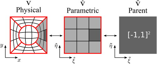
For the example of a 2D pin-cell constructed from five bi-quadratic NURBS patches, the schematic in Figure 1, created by Wilson et al. presents the domain of a single NURBS patch as that represented in the three classical spaces of IGA; viz. the real physical, the parametric and the parent spaces (Wilson, Eaton, and Kópházi 2024). The exact representation of the underlying geometry is maintained as the mesh is refined because the geometrical mapping and the Jacobian are invariant under refinement (Piegl and Tiller 1997). However, this should not be confused for being piecewise constant.

Figure 1. An example of a 2D pin-cell represented by bi-quadratic NURBS patches (macro-elements) in the real physical space, $V,$ as denoted by the parameters x and y (Wilson, Eaton, and Kópházi 2024). The domain, represented in the parametric space, $\widehat{V},$ is formed from the tensor-product of two 1D spaces, as denoted by the parameters $\widehat{\xi }$ and $\widehat{\eta }.$ The parametric space has been decomposed into non-vanishing knot-spans (micro-elements), over which, numerical integration is performed by an affine mapping from the parent domain, $\tilde{V},$ as denoted by the parameters $\tilde{\xi }$ and $\tilde{\eta }.$ The patch boundaries are highlighted in red; whereas the non-vanishing knot-spans within a patch are separated by black lines. The image of given non-vanishing knot-span, shaded in dark grey, can be represented in all three spaces. (V. the web-based version for reference to color.).

One way in which to enrich the parametric domain, as suggested by Figure 1, is to form additional non-zero-knot-spans. Knots can be inserted with a multiplicity of one, KI-1-refinement, up to $p+1,$ KI-h-refinement. The latter is analogous to h-refinement in a standard FEM because the basis is reduced to $C^0$-continuity across the newly-formed element boundaries. Another way in which to enrich the basis is by degree-elevation (DE), which is analagous to p-refinement in a standard FEM. One notes that the refinement processes of KI and DE are not commutative (Cottrell, Hughes, and Reali 2007).

2.1. Degeneracy

Multi-patch configurations are convenient for assigning different material properties to the different regions of a problem. Moreover, the tensor-product structure of the NURBS parametric space can complicate the analysis over free-form geometries constructed from too few patches because they can become very distorted. In extreme cases, the geometrical mapping can become singular. Any derivatives of the NURBS basis functions, with respect to the real physical space, can be determined from the chain rule; and one must call upon entries from the inverse of the volumetric Jacobian matrix, ${[{\underset{=}{\mathbf{J}}}_V]}^{-1}.$ There exist explicit expressions for the inversion of $2\times 2$ and $3\times 3$ matrices; e.g. the inverse of the 2D Jacobian matrix: (8) $${\left[{\underset{=}{\mathbf{J}}}_V\right]}^{-1}=\left[\begin{array}{cc}\frac{d\xi }{\mathit{\text{dx}}}& \frac{d\eta }{\mathit{\text{dx}}}\\ \frac{d\xi }{\mathit{\text{dy}}}& \frac{d\eta }{\mathit{\text{dy}}}\end{array}\right]=\frac{1}{\mathrm{\text{det}}{\underset{=}{\mathbf{J}}}_V}\left[\begin{array}{cc}\frac{\mathit{\text{dy}}}{d\eta }& -\frac{\mathit{\text{dy}}}{d\xi }\\ -\frac{\mathit{\text{dx}}}{d\eta }& \frac{\mathit{\text{dx}}}{d\xi }\end{array}\right].$$(8)

Clearly, ${[{\underset{=}{\mathbf{J}}}_V]}^{-1}$ is not defined when the gradient of the mapping, or rather its determinant, becomes negligibly small; v. Figure 2. Yet, this is may not be to the detriment of the numerical method; viz. when formulating integral quantities by Gaussian quadrature rules, the evaluation points may not coincide with any point of singularity (Beer 2015). Moreover, Galerkin discretizations are typically well-conditioned and the resulting volumetric mass matrices, or Gram matrices of category 0, and the stiffness matrices are diagonally dominant for all practical numerical quadrature sets (Cottrell, Hughes, and Bazilevs 2009).

Figure 2. The Jacobian determinant for the example of a 2D unit circle as represented by a single degenerate bi-quadratic NURBS patch (left) and five non-degenerate bi-quadratic NURBS patches (right). The geometrical mapping is non-invertible at the corners of the circle on the left-hand side where the Jacobian determinant becomes negligibly small. (V. the web-based version for reference to color.).

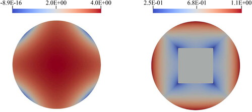
On the contrary, degenerate patches are not suitable for discretizations that require $\overrightarrow{\nabla }R$ to be (square-)integrable over the boundary, $\partial V_e.$ This is exactly where the singularities lie in the case of a 2D circle represented by a single bi-quadratic NURBS patch; v. Figure 2 and q.v. Section 5.2. Since the parametrization is invariant under refinement, any problems associated with degeneracy could only be rectified by a better coarsest mesh.

Indeed, an isoparametric element performs best when it resembles its unmapped shape; viz. upper-bounds and lower-bounds are generally imposed upon the interior angles or the aspect ratio of triangular and quadrilateral elements, respectively (Arnold 1982). Similarly, the coarsest mesh for any problem considered in this work is formed from NURBS patches with distinct edges and surfaces, as per an equivalent hypercube topology in the parametric space. For example, a circle is represented by five non-degenerate patches instead of a degenerate one.

2.2. Energy-dependent meshes

The microscopic neutron cross-section data can vary significantly across the range of possible neutron energies. Therefore, the spatial variation in the scalar neutron flux can also vary significantly across the different neutron energy groups. In order to address this issue, Wilson et al. present a numerical approach for solving the multi-group NDE over energy-dependent meshes derived from some common coarsest-mesh description (Wilson, Eaton, and Kópházi 2024).

One should expect to be able to maximize the accuracy per total DoF by solving the multi-group NTE over separate energy-dependent meshes, ${\mathcal{T}}^g(V),$ and their respective function spaces, ${\widehat{\mathcal{V}}}_{h,p}^g,$ which may be refined independently; i.e., $G\times \mathrm{\text{dim\hspace{0.17em}}}{\widehat{\mathcal{V}}}_{h,p}>\sum {}_g\mathrm{\text{\hspace{0.17em}\hspace{0.17em}dim\hspace{0.17em}}}{\widehat{\mathcal{V}}}_{h,p}^g.$

The group-to-group neutron scattering and fission sources are calculated as the conservative interpolation onto a super-mesh, which is formed as the intersection of two implicated meshes (Farrell and Maddison 2011). Choosing the weighted-residual formulation to be optimal in the $H^1$-norm, the orthogonal Galerkin projection of a discrete field onto the function spaced spanned by a target basis can be expressed in matrix form: (9a) $$[{\underset{=}{S}}_V^{\mathit{\text{tt}}}+{\underset{=}{M}}_V^{\mathit{\text{tt}}}]·{\underset{¯}{v}}^t=[{\underset{=}{S}}_V^{\mathit{\text{td}}}+{\underset{=}{M}}_V^{\mathit{\text{td}}}]·{\underset{¯}{v}}^d\text{;}$$(9a) (9b) $$\Rightarrow {\underset{=}{K}}_V^{\mathit{\text{tt}}}·{\underset{¯}{v}}^t={\underset{=}{K}}_V^{\mathit{\text{td}}}·{\underset{¯}{v}}^d\text{;}$$(9b) where the consistent mass and stiffness matrices, ${\underset{=}{M}}_V^{\mathit{\text{tt}}}$ and ${\underset{=}{S}}_V^{\mathit{\text{tt}}},$ respectively, are formed by integrating the product of those functions, defined over ${\mathcal{T}}^t,$ that belong to the target function space, ${\widehat{\mathcal{V}}}_{h,p}^t.$ Whereas the projective mass and stiffness matrices, ${\underset{=}{M}}_V^{\mathit{\text{td}}}$ and ${\underset{=}{S}}_V^{\mathit{\text{td}}},$ respectively, require that in the same integrand are evaluated the product of functions defined over different spatial meshes, ${\mathcal{T}}^t$ and ${\mathcal{T}}^d,$ that belong to different function spaces, ${\widehat{\mathcal{V}}}_{h,p}^t$ and ${\widehat{\mathcal{V}}}_{h,p}^d,$ respectively.

Now, some function may undergo a change of basis transformation by pre-multiplying the control-variables, ${\underset{¯}{v}}^d,$ by the combined transfer matrix, ${\underset{=}{K}}_V^{t\leftarrow d},$ for which the interpolation of the function from a donor mesh onto a target mesh, is optimal with respect to the $H^1$-norm. Although ${\underset{=}{S}}_V^{\mathit{\text{tt}}}$ is singular, ${\underset{=}{K}}_V^{\mathit{\text{tt}}}$ is symmetric-positive definite; and therefore, it is readily invertible using standard iterative smoothers: (10a) $${\underset{¯}{v}}^t={\left[{\underset{=}{K}}_V^{\mathit{\text{tt}}}\right]}^{-1}·{\underset{=}{K}}_V^{\mathit{\text{td}}}·{\underset{¯}{v}}^d,$$(10a) (10b) $$=\underset{(N^t\times N^d)(N^d\times 1)}{{\underset{=}{K}}_V^{\mathit{\text{t←d}}}·{\underset{¯}{v}}^d.}$$(10b)

Owing to the local formulation of discontinuous Galerkin discretizations, it is not necessary to assemble large matrices since the above equations can be formulated locally; and thus, ${\underset{=}{K}}_V^{\mathit{\text{tt}}}$ can be inverted locally; e.g. using efficient LAPACK routines such as DGETRF and DGETRI.

 The interpolation of a discrete scalar field between meshes is not unique in its application to energy-dependent meshes. It is also employed in the next section when evaluating the interpolation-based error measures that drive the adaptive refinement strategies.

3. The adaptive mesh refinement (AMR) strategies

Within a common computational framework, Wilson et al. present two different interpolation-based AMR-h(p) strategies for a constraint-based continuous Bubnov-Galerkin (CBG-)IGA spatial discretization of the multi-group NDE (Wilson, Eaton, and Kópházi 2024). The first aims to minimize, almost everywhere, the discretization error in the solution, as measured in an appropriate norm. This is called the energy-driven (NRG-)AMR strategy, although the error does not have to be measured in the energy-norm; viz. the $L_2$-norm or the $H^1$-(semi-)norm. The second strategy aims to minimize the error in some specific goal. This is called the goal-based (DWR-) AMR strategy. Neither strategy considers mesh coarsening.

The work presented in this paper adopts the same AMR-h(p) framework to establish interpolation-based NRG and DWR error measures for an SIP-DG IGA spatial discretization of the multi-group NDE. Within a given AMR iteration, the multi-group components of the numerical solution must be known in order to evaluate the global error in the QoI, ${ϵ}^{(i)},$ as measured in an appropriate norm: (11) $${ϵ}^{(i)}=\Vert \mathit{\text{QoI}}(\varphi )-\mathit{\text{QoI}}({\widehat{\varphi }}_{h,p}^{(i)})\Vert .$$(11)

The QoI represents a physical quantity such as the scalar neutron flux or fluence at a point in the domain or averaged over a region.

Mesh optimality is achieved by maximizing the decrease in the global error, $\Delta {ϵ}^{(i)},$ between successive iterations, per increase in the number of unknowns, $\Delta \mathit{\text{Do}}{F}^{(i)}.$

The mechanisms for spatial refinement are restricted to isotropic DE-1-refinement and isotropic KI-h-refinement; i.e., $h^{*},p^{*}=\{h/2,p\text{or}h,p+1\}.$ This is comparable to a standard AMR-h(p) strategy for a classical FEM. It is important to note that the cost of performing KI-h-refinement becomes increasingly more expensive as the polynomial degree of the basis, p, increases. This is due to the fact that the number of unknowns is increased for every knot inserted; and knots must be inserted with a multiplicity of $\dot{m}=p+1$ in order to render the basis discontinuous.

Discontinuous discretizations naturally allow for arbitrary local refinement of the mesh because the approximation space is discontinuous by definition. However, regardless of regularity, continuity must always be enforced across the physical space in a weak sense. In the limit of a discontinuous basis, one can also exploit the efficient and well-established pre-conditioners that have been developed for low-order continuity FEMs, which are not generally effective for bases that exhibit higher-order continuity (Gahalaut, Kraus, and Tomar 2013; Sangalli and Tani 2016).

Moreover, the tensor-product structure of the NURBS patches lends itself to the cell-based approach adopted by Wang and Ragusa (Wang, Bangerth, and Ragusa 2009). In this approach, any local isotropic h-refinement consists of bisecting an element in each parametric direction forming $2^d$ new elements, for $d=2,3.$ Therefore, the AMR procedure can proceed as a sequence of adapted meshes that belong to a hierarchy of nested meshes (Wilson, Eaton, and Kópházi 2024).

A numerical reference solution, ${\widehat{\varphi }}_{\mathit{\text{ref}}},$ is proposed in lieu of the true solution, $\varphi .$ The reference solution must sufficiently resolve the local scales of either of the two proposed local-refinement options, KI-h-refinement and DE-1-refinement, in order to justify the use of one over the other in the next iteration of mesh refinement; i.e., ${\widehat{\mathcal{V}}}_{h^{*},p^{*}}(V_e)\subset {\widehat{\mathcal{V}}}_{\mathit{\text{ref}}}(V_e),$ (Demkowicz 2007). Accordingly, the reference mesh should be at least one-level of uniform KI-h-refinement and DE-1-refinement above that of the coarser current mesh; where ${\mathcal{T}}_{\mathit{\text{ref}}}={\mathcal{T}}_{\text{h/2},p\text{+1}}$ and therefore, ${\widehat{\varphi }}_{\mathit{\text{ref}}}={\widehat{\varphi }}_{\text{h/2},p\text{+1}}\in {\widehat{\mathcal{V}}}_{\text{h/2},p\text{+1}}.$ All measurements of error are now estimates made with respect to the reference solution; i.e., $\widehat{ϵ}=|\widehat{e}{|}_{{\mathit{\hspace{0.17em}H}}^1},$ where $\widehat{e}={\widehat{\varphi }}_{\mathit{\text{ref}}}-{\widehat{\varphi }}_{h,p}.$

For ${\widehat{\varphi }}_{\mathit{\text{ref}}}\in {\widehat{\mathcal{V}}}_{\mathit{\text{ref}}}$ and for ${\widehat{\varphi }}_{h,p}\in {\widehat{\mathcal{V}}}_{h,p}\subset {\widehat{\mathcal{V}}}_{\mathit{\text{ref}}}$ it can be shown that the global error estimate, $\widehat{ϵ},$ provides an upper-bound to the true global error, under the assumption that the reference solution is a much better approximation of the true solution than is ${\widehat{\varphi }}_{h,p}$ calculated on ${\mathcal{T}}_{h,p};$ i.e., $\Vert \varphi -{\widehat{\varphi }}_{\mathit{\text{ref}}}\Vert \ll \Vert {\widehat{\varphi }}_{\mathit{\text{ref}}}-{\widehat{\varphi }}_{h,p}\Vert$ (Wilson 2021).

It would be computationally expensive to perform two explicit calculations over two different levels of mesh refinement for each energy group. Fortunately, one can invoke Strang‘s Second Lemma of quasi-best approximation, for non-conforming and consistent discretizations, to demonstrate that the chosen approximation space yields a solution, ${\widehat{\varphi }}_{h,p}\in {\widehat{\mathcal{V}}}_{h,p},$ whose error is bounded by the quasi-best approximation error. The quasi-best approximation error is bounded by the difference in the exact solution and any function that belongs to the finite-dimensional hp function space. In particular, one chooses the projection of the exact solution onto this approximation space, $\prod {}_{h,p}\varphi .$ Therefore, the entire AMR procedure can be driven by controlling the interpolation error that bounds the quasi-best approximation error, which, in turn, bounds the true discretization error (Demkowicz 2004).

Substitution of the exact solution for the reference solution yields an an iterative procedure that requires the numerical solution over a more-refined reference mesh and its projection onto a coarser current mesh. This projection, $\prod {}_{h,p}:{\widehat{\mathcal{V}}}_{\text{h/2},p\text{+1}}\to {\widehat{\mathcal{V}}}_{h,p},$ is performed as a conservative interpolation between volume meshes. As an approximation, $\widehat{\varphi },$ is sought to minimize the discretization error as that measured in the energy-norm, or the $H^1$-(semi)norm by the equivalence of norms, unsurprisingly, the interpolation over the reference solution onto the coarser mesh is chosen to be optimal in the $H^1$-norm.

Driven by the residual in the interpolation-based error estimate, successive meshes at each iteration of the AMR procedure are obtained by minimizing local contributions to the global error. An element is flagged if its local contribution to the global error is greater than some threshold, which is taken as some fraction of the maximum error over a single element belonging to any of the current coarser meshes.

4. The multi-group neutron diffusion equation

The research presented in this paper considers the steady-state, energy-dependent, neutron diffusion equation (NDE). The spatial domain is discretized using isogeometric analysis (IGA); and the energy domain is discretized using the multi-group approximation.

The continuous energy domain, $(E_{\mathrm{\text{min}}},E_{\mathrm{\text{max}}}],$ is partitioned into distinct values, $E_{\mathrm{\text{max}}}=E_0>E_1>\dots >E_G=E_{\mathrm{\text{min}}},$ forming G number of energy groups; such that the $g^{\mathit{\text{th}}}$-group spans the half-closed interval $(E_g,E_{g-1}].$ Any integrals over the entire energy spectrum are expressed as a sum of individual integrals over each energy group; i.e.,: (12) $${\int }_0^{\infty }dE\approx {\int }_{E_G}^{E_0}dE\Rightarrow \sum _{g=1}^G{\int }_{E_g}^{E_{g-1}}\mathit{\text{dE}}.$$(12)

The defining equation is integrated over each energy group and the result is solved for the multi-group components of the scalar neutron flux, ${\varphi }^g;$ where: (13) $${\varphi }^g(\overrightarrow{r})={\int }_{E_g}^{E_{g-1}}\varphi (\overrightarrow{r},E)\mathit{\text{dE}}.$$(13)

4.1. The direct (primal) equation

The direct (primal) multi-group NDE is posed on the closure of a connected and bounded domain, $V\subset {\mathbb{R}}^d,$ in d-dimensional Euclidean space for d = 2, 3. The strong form of the problem is cast as solving ${\varphi }^g:V\to \mathbb{R}$ for $g=1,\dots ,G:$ $$\{\begin{array}{lll}-\overrightarrow{\nabla }·D^g(\overrightarrow{r})\overrightarrow{\nabla }{\varphi }^g(\overrightarrow{r})+{\Sigma }_r^g(\overrightarrow{r}){\varphi }^g(\overrightarrow{r})=q^g(\overrightarrow{r}),\hfill & \overrightarrow{r}\in V\text{;}\hfill & \hfill \mathrm{(}\text{14a}\mathrm{)}\\ \hfill {\varphi }^g(\overrightarrow{r})=g_D^g,& \overrightarrow{r}\in \partial V_D\text{;}\hfill & \hfill (14\mathrm{b})\\ \hfill \overrightarrow{\nabla }{\varphi }^g(\overrightarrow{r})·\overrightarrow{n}(\overrightarrow{r})=g_N^g,& \overrightarrow{r}\in \partial V_N\text{;}\hfill & \hfill \mathrm{(}\text{14c}\mathrm{)}\end{array}$$ where Dirichlet and Neumann-type BCs, Equation 14b$$\{\begin{array}{lll}-\overrightarrow{\nabla }·D^g(\overrightarrow{r})\overrightarrow{\nabla }{\varphi }^g(\overrightarrow{r})+{\Sigma }_r^g(\overrightarrow{r}){\varphi }^g(\overrightarrow{r})=q^g(\overrightarrow{r}),\hfill & \overrightarrow{r}\in V\text{;}\hfill & \hfill \mathrm{(}\text{14a}\mathrm{)}\\ \hfill {\varphi }^g(\overrightarrow{r})=g_D^g,& \overrightarrow{r}\in \partial V_D\text{;}\hfill & \hfill (14\mathrm{b})\\ \hfill \overrightarrow{\nabla }{\varphi }^g(\overrightarrow{r})·\overrightarrow{n}(\overrightarrow{r})=g_N^g,& \overrightarrow{r}\in \partial V_N\text{;}\hfill & \hfill \mathrm{(}\text{14c}\mathrm{)}\end{array}$$ and Equation 14c$$\{\begin{array}{lll}-\overrightarrow{\nabla }·D^g(\overrightarrow{r})\overrightarrow{\nabla }{\varphi }^g(\overrightarrow{r})+{\Sigma }_r^g(\overrightarrow{r}){\varphi }^g(\overrightarrow{r})=q^g(\overrightarrow{r}),\hfill & \overrightarrow{r}\in V\text{;}\hfill & \hfill \mathrm{(}\text{14a}\mathrm{)}\\ \hfill {\varphi }^g(\overrightarrow{r})=g_D^g,& \overrightarrow{r}\in \partial V_D\text{;}\hfill & \hfill (14\mathrm{b})\\ \hfill \overrightarrow{\nabla }{\varphi }^g(\overrightarrow{r})·\overrightarrow{n}(\overrightarrow{r})=g_N^g,& \overrightarrow{r}\in \partial V_N\text{;}\hfill & \hfill \mathrm{(}\text{14c}\mathrm{)}\end{array}$$, respectively, are prescribed on the external boundaries; i.e., $\partial V_{\mathit{\text{ext}}}=\partial V_D\cup \partial V_N,$ respectively; and the normal vector, $\overrightarrow{n},$ is outward-pointing. The defining equations can be recast in block-like group operator notation: (15a) $$L\varphi =q,$$(15a) (15b) $$=S\varphi +F\varphi +q_x\text{;}$$(15b) with the scalar neutron flux, $\varphi ={[{\varphi }^1,\dots ,{\varphi }^G]}^T;$ the extraneous fixed-sources, $q_x={[q_x^1,\dots ,q_x^G]}^T;$ the diagonal loss operator, L, which comprises within-group losses due to diffusive-leakage and total collision, $L^g,$ Equation 16a(16a) $$L^g\varphi :=-\overrightarrow{\nabla }·D^g\overrightarrow{\nabla }{\varphi }^g+{\Sigma }_r^g{\varphi }^g\text{;}$$(16a) ; the scatter operator, S, which comprises group-to-group scatter terms, $S^g,$ Equation 16b(16b) $$S^g\varphi :=\sum _{g\prime \ne g}{\Sigma }_s^{g\prime \to g}{\varphi }^{g\prime }\text{;}$$(16b) ; and the fission operator, F, which comprises multi-group fission terms, $F^g,$ Equation 16c(16c) $$F^g\varphi :={\chi }^g\sum _{g\prime }{\nu }^{g\prime }{\Sigma }_f^{g\prime }{\varphi }^{g\prime }.$$(16c) . (16a) $$L^g\varphi :=-\overrightarrow{\nabla }·D^g\overrightarrow{\nabla }{\varphi }^g+{\Sigma }_r^g{\varphi }^g\text{;}$$(16a) (16b) $$S^g\varphi :=\sum _{g\prime \ne g}{\Sigma }_s^{g\prime \to g}{\varphi }^{g\prime }\text{;}$$(16b) (16c) $$F^g\varphi :={\chi }^g\sum _{g\prime }{\nu }^{g\prime }{\Sigma }_f^{g\prime }{\varphi }^{g\prime }.$$(16c)

Defining the operator, A, such that: (17) $$A\varphi =(L-S)\varphi ,$$(17) one can distinguish fixed-source problems: (18) $$(A-F)\varphi =q_x,$$(18) from eigenvalue ones: (19) $$A\varphi =\frac{1}{{\mathrm{k}}_{\text{eff}}}F\varphi .$$(19)

4.2. The adjoint (dual) equation

Mathematically, the dual problem should be adjoint-consistent with the primal with respect to the discretization of the spatial and energy domains. By linearity of the inner-product, adjoint-consistency can be satisfied in each of the operators defined in Equation 16(16a) $$L^g\varphi :=-\overrightarrow{\nabla }·D^g\overrightarrow{\nabla }{\varphi }^g+{\Sigma }_r^g{\varphi }^g\text{;}$$(16a) ; i.e., (Lewis and Miller 1984): (20) $$\sum _{g=1}^G[{\int }_V{\varphi }^{g†}(\overrightarrow{r})B^g{\varphi }^g(\overrightarrow{r})\mathit{\text{ dV}}]\equiv \sum _{g=1}^G[{\int }_V{\varphi }^g(\overrightarrow{r})B^{g†}{\varphi }^{g†}(\overrightarrow{r})\mathit{\text{ dV}}].$$(20)

The dual problem is posed in the same domain, $V\in {\mathbb{R}}^d,$ as the primal one; its strong form cast in multi-group operator notation as finding ${\varphi }^{g†}:V\to \mathbb{R}$ for $g=G,\dots ,1:$ (21a) $$L^{†}{\varphi }^{†}=q^{†},$$(21a) (21b) $$=S^{†}{\varphi }^{†}+F^{†}{\varphi }^{†}+q_x^{†}\text{;}$$(21b) with the scalar neutron importance, ${\varphi }^{†}={[{\varphi }^{1†},\dots ,{\varphi }^{G†}]}^T;$ the adjoint source, $q_x^{†}={[q_x^{1†},\dots ,q_x^{G†}]}^T;$ and the loss, scatter and fission adjoint operators, $L^{†},S^{†}$ and $F^{†},$ respectively: (22a) $$L^{g†}{\varphi }^{†}:=-\overrightarrow{\nabla }·D^g\overrightarrow{\nabla }{\varphi }^{g†}+{\Sigma }_r^g{\varphi }^{g†}\text{;}$$(22a) (22b) $$S^{g†}{\varphi }^{†}:=\sum _{g\prime \ne g}{\Sigma }_s^{g\to g\prime }{\varphi }^{g\prime }\text{;}$$(22b) (22c) $$F^{g†}{\varphi }^{†}:={\nu }^g{\Sigma }_f^g\sum _{g\prime }{\chi }^{g\prime }{\varphi }^{g\prime }.$$(22c)

The scatter and the fission operators are not self-adjoint; their adjoint operators are obtained by transposition and the interchanging of arguments of the energy-integral kernels (Schunert et al. 2015). The loss operator is formally self-adjoint, $(L\varphi ,{\varphi }^{†})=(\varphi ,L{\varphi }^{†});$ however, the diffusive-leakage term necessitates an appropriate prescription of adjoint BCs. It simplifies the problem to restrict the general Dirichlet and Neumann BCs, Equation 14b and Equation 14c, respectively, to a certain few that are commonly used in reactor physics and radiation shielding problems. For the set of zero-flux, reflective and vacuum BCs, prescribed on the external boundaries, $\partial V_0,\partial V_R$ and $\partial V_V$ respectively: $$\{\begin{array}{cc}{\varphi }^g(\overrightarrow{r})=0,& \overrightarrow{r}\in \partial V_0\text{;\hspace{1em}\hspace{1em}}\mathrm{(}\text{23a}\mathrm{)}\\ -D^g(\overrightarrow{r})\overrightarrow{\nabla }{\varphi }^g(\overrightarrow{r})·\overrightarrow{n}=0,\hfill & \overrightarrow{r}\in \partial V_R\text{;\hspace{1em}\hspace{1em}}\mathrm{(}\text{23b}\mathrm{)}\hfill \\ -D^g(\overrightarrow{r})\overrightarrow{\nabla }{\varphi }^g(\overrightarrow{r})·\overrightarrow{n}=\frac{1}{2}{\varphi }^g(\overrightarrow{r}),\hfill & \overrightarrow{r}\in \partial V_V.(23\mathrm{c})\hfill \end{array}$$

The corresponding set of adjoint BCs are prescribed over the same boundaries: $$\{\begin{array}{cc}{\varphi }^{g†}(\overrightarrow{r})=0,& \overrightarrow{r}\in \partial V_0\text{;\hspace{1em}\hspace{1em}}\mathrm{(}\text{24a}\mathrm{)}\\ D^g(\overrightarrow{r})\overrightarrow{\nabla }{\varphi }^{g†}(\overrightarrow{r})·\overrightarrow{n}=0,\hfill & \overrightarrow{r}\in \partial V_R\text{;\hspace{1em}\hspace{1em}}\mathrm{(}\text{24b}\mathrm{)}\hfill \\ D^g(\overrightarrow{r})\overrightarrow{\nabla }{\varphi }^{g†}(\overrightarrow{r})·\overrightarrow{n}=\frac{-1}{2}{\varphi }^{g†}(\overrightarrow{r}),\hfill & \overrightarrow{r}\in \partial V_V\text{; \hspace{1em}\hspace{1em}}\mathrm{(}\text{24c}\mathrm{)}\hfill \end{array}$$ where the vacuum BC has been considered as a general Robin BC of the form: $\alpha \varphi +\overrightarrow{\nabla }\varphi ·\overrightarrow{n}=g,$ which assumes that the incoming partial current of neutrons, as well as the outgoing partial current of neutron importance, are both negligibly small.

In a similar manner to Equation 17(17) $$A\varphi =(L-S)\varphi ,$$(17) for the primal problem, the operator $A^{†}$ is defined such that: (25) $$A^{†}{\varphi }^{†}=(L^{†}-S^{†}){\varphi }^{†}.$$(25)

Again, one distinguishes fixed-source problems: (26) $$(A^{†}-F^{†}){\varphi }^{†}=q_x^{†},$$(26) from eigenvalue ones: (27) $$A^{†}{\varphi }^{†}=\frac{1}{{\mathrm{k}}_{\text{eff}}^{†}}{F}^{†}{\varphi }^{†}.$$(27)

Under the assumption that the property of (semi-discrete) adjoint-consistency holds, it should be clear that ${\mathrm{k}}_{\text{eff}}^{†}={\mathrm{k}}_{\text{eff}};$ i.e., the Rayleigh quotient: (28) $${\mathrm{k}}_{\text{eff}}^{†}=\frac{(\varphi ,F^{†}{\varphi }^{†})}{(\varphi ,A^{†}{\varphi }^{†})}=\frac{(F\varphi ,{\varphi }^{†})}{(A\varphi ,{\varphi }^{†})}={\mathrm{k}}_{\text{eff}}\text{;}$$(28) where $|1/{\mathrm{k}}_{\text{eff}}|$ is determined after each ${(i)}^{\mathit{\text{th}}}$ power-iteration: (29a) $${\mathrm{k}}_{\text{eff}}^{(i)}=\frac{(F{\varphi }^{(i)},{\varphi }^{†})}{(A{\varphi }^{(i)},{\varphi }^{†})}=\frac{(F{\varphi }^{(i)},{\varphi }^{†})}{\frac{1}{k_{\text{eff}}^{(i+1)}}(F{\varphi }^{(i+1)},{\varphi }^{†})}\text{;}$$(29a) (29b) $$\Rightarrow \frac{1}{{\mathrm{k}}_{\text{eff}}^{(i+1)}}=\frac{1}{{\mathrm{k}}_{\text{eff}}^{(i)}}\frac{(F{\varphi }^{(i)},{\varphi }^{†})}{(F{\varphi }^{(i+1)},{\varphi }^{†})}\text{;}$$(29b) where ${\varphi }^{†}$ is not obliged to be the solution to the adjoint problem in the above iteration; and $\underset{(i)\to \infty }{\mathrm{\text{lim}}}{\mathrm{k}}_{\text{eff}}^{(i)}={\mathrm{k}}_{\text{eff}}.$

5. An interior penalty scheme for a discontinuous Galerkin isogeometric discretization

One seeks to approximate the (semi-)analytic solution by some finite linear combination of basis functions and expansion coefficients. In the interest of discontinuous formulations, it is appropriate to exploit the usual space of functions in a piecewise manner. The broken Sobolev space, $H^s(\mathcal{T}),$ defines a set of spaces, $H^s(V_e),$ spanned by locally supported functions that belong to the regular Sobolev space, in the restriction to $V_e:$ (30) $$H^s(\mathcal{T}):=\{u\in L_2(V):u{|}_{V_e}\in H^s(V_e),\forall V_e\in \mathcal{T}(V)\}\text{;}$$(30) where the usual Sobolev embeddings rules apply; i.e.,, $H^{s+1}(\mathcal{T})\subset H^s(\mathcal{T}).$ The associated broken inner-product and broken norm, are given below in Equation 31a(31a) $${(u,v)}_{H^s(\mathcal{T})}\mathrm{}:=\text{}\sum _{V_e\in \mathcal{T}(V)}\text{}{(u,v)}_{H^s(V_e)}\text{;}$$(31a) and Equation 31b(31b) $$\Vert u{\Vert }_{H^s(\mathcal{T})}\mathrm{}:={(u,u)}_{H^s(\mathcal{T})}^{\text{1/2}}.$$(31b) , respectively: (31a) $${(u,v)}_{H^s(\mathcal{T})}\mathrm{}:=\text{}\sum _{V_e\in \mathcal{T}(V)}\text{}{(u,v)}_{H^s(V_e)}\text{;}$$(31a) (31b) $$\Vert u{\Vert }_{H^s(\mathcal{T})}\mathrm{}:={(u,u)}_{H^s(\mathcal{T})}^{\text{1/2}}.$$(31b)

The restriction of such functions and their normal derivatives with support over V_e are defined over $\partial V_e$ by trace operators, ${\gamma }_i:H^s(V_e)\to H^{s-i-1/2}(\partial V_e)$ for $0\le i<s$ (Oden and Reddy 2011). Of particular interest are the Dirichlet trace, ${\gamma }_0,$ and the Neumann trace, ${\gamma }_1,$ which are well defined in $L_2(\partial V_e)$ for $s>\text{3/2}:$ (32a) $${\gamma }_{0}u:=u{|}_{\partial V_e}\text{;}$$(32a) (32b) $${\gamma }_{1}u:=\overrightarrow{\nabla }u·\overrightarrow{n}{|}_{\partial V_e}.$$(32b)

Any function $u\in H^s(\mathcal{T})$ is discontinuous, along with its normal derivatives, across element interfaces. Therefore, one defines the gradient operator in an element-wise manner; i.e., the broken gradient: (33) $$(\overrightarrow{\nabla }u){|}_{V_e}:=\overrightarrow{\nabla }(u{|}_{V_e}),\hspace{1em}\forall V_e\in \mathcal{T}(V).$$(33)

For some function $u\in H^s(V),$ for $s\ge 1,$ where any jump in u is always negligibly small, the broken gradient coincides with the gradient defined in a distributional sense; i.e., $(\overrightarrow{\nabla }u){|}_{V_e}=\overrightarrow{\nabla }u.$ Such a function also belongs to the broken Sobolev space, $u\in H^s(\mathcal{T}),$ where it is not required for any jump in u to be negligibly small. Therefore, one can assume that $H^s(V)\subset H^s(\mathcal{T});$ or rather, under some assumption of regularity, only sufficiently smooth solutions belong to $H^s(V)$ (Di Pietro and Ern 2012). This may explain any observed increase in accuracy for (S)IP-DG discretizations of elliptic problems over standard continuous Bubnov-Galerkin (CBG) ones over the same mesh (Kaplan 1969; Wilson et al. 2018).

It is useful to provide a formal definition of the jump in a function, as well as the average across an interface, $\partial V_f\in \partial V_{\mathit{\text{int}}};$ where for $s>\text{3/2},$ the domain is smooth enough to admit two-valued traces. Although arbitrary, the definitions are perspective-dependent. The superscript (+) pertains to the active-element, $V_{+},$ whose outward-pointing normal vector over its boundary, ${\overrightarrow{n}}^{+},$ coincides with that, $\overrightarrow{n},$ at the interface, $V_{+}\cap V_{-};$ whereas the superscript (-) pertains to the neighbor-element, $V_{-},$ whose outward-pointing normal vector over its boundary, ${\overrightarrow{n}}^{-},$ has the opposite orientation to that of the active-element; i.e., $\overrightarrow{n}={\overrightarrow{n}}^{+}=-{\overrightarrow{n}}^{-}.$ The jump, ${[[·]]}_{\partial V_f},$ and the average, ${\left\{\right\{·\left\}\right\}}_{\partial V_f},$ are defined for some scalar-valued function, u, in Equation 34a$$\begin{array}{l}{\left[\right[u\left]\right]}_{\partial V_f}:=\{\begin{array}{cc}{u}^{+}-u^{-},\hspace{1em}\mathrm{\hspace{1em}}\mathrm{\hspace{1em}}\hfill & \forall \partial V_f\in \partial V_{\mathit{\text{int}}}\text{;}\hfill \\ u,\hspace{1em}\mathrm{\hspace{1em}}\mathrm{\hspace{1em}}\hfill & \forall \partial V_f\in \partial V_{\mathit{\text{ext}}}\text{;}\hfill \end{array}(34\mathrm{a})\\ {\left\{\right\{u\left\}\right\}}_{\partial V_f}:=\{\begin{array}{cc}\frac{1}{2}(u^{+}+u^{-}),\hspace{1em}\hfill & \forall \partial V_f\in \partial V_{\mathit{\text{int}}}\text{;}\hfill \\ u,\hspace{1em}\hfill & \forall \partial V_f\in \partial V_{\mathit{\text{ext}}}.\hfill \end{array}(34\mathrm{b})\end{array}$$ and Equation 34b$$\begin{array}{l}{\left[\right[u\left]\right]}_{\partial V_f}:=\{\begin{array}{cc}{u}^{+}-u^{-},\hspace{1em}\mathrm{\hspace{1em}}\mathrm{\hspace{1em}}\hfill & \forall \partial V_f\in \partial V_{\mathit{\text{int}}}\text{;}\hfill \\ u,\hspace{1em}\mathrm{\hspace{1em}}\mathrm{\hspace{1em}}\hfill & \forall \partial V_f\in \partial V_{\mathit{\text{ext}}}\text{;}\hfill \end{array}(34\mathrm{a})\\ {\left\{\right\{u\left\}\right\}}_{\partial V_f}:=\{\begin{array}{cc}\frac{1}{2}(u^{+}+u^{-}),\hspace{1em}\hfill & \forall \partial V_f\in \partial V_{\mathit{\text{int}}}\text{;}\hfill \\ u,\hspace{1em}\hfill & \forall \partial V_f\in \partial V_{\mathit{\text{ext}}}.\hfill \end{array}(34\mathrm{b})\end{array}$$, respectively: $$\begin{array}{l}{\left[\right[u\left]\right]}_{\partial V_f}:=\{\begin{array}{cc}{u}^{+}-u^{-},\hspace{1em}\mathrm{\hspace{1em}}\mathrm{\hspace{1em}}\hfill & \forall \partial V_f\in \partial V_{\mathit{\text{int}}}\text{;}\hfill \\ u,\hspace{1em}\mathrm{\hspace{1em}}\mathrm{\hspace{1em}}\hfill & \forall \partial V_f\in \partial V_{\mathit{\text{ext}}}\text{;}\hfill \end{array}(34\mathrm{a})\\ {\left\{\right\{u\left\}\right\}}_{\partial V_f}:=\{\begin{array}{cc}\frac{1}{2}(u^{+}+u^{-}),\hspace{1em}\hfill & \forall \partial V_f\in \partial V_{\mathit{\text{int}}}\text{;}\hfill \\ u,\hspace{1em}\hfill & \forall \partial V_f\in \partial V_{\mathit{\text{ext}}}.\hfill \end{array}(34\mathrm{b})\end{array}$$

To allow for compact notation, the jumps and averages over those boundaries that lie adjacent to the physical boundary, $\partial V_{\mathit{\text{ext}}},$ have been included above.

Physically, the solution to the primal problem is assumed to be sufficiently smooth that any jumps in the scalar neutron flux, $\varphi ,$ and any jumps in the normal component of the net neutron current, $-D\overrightarrow{\nabla }\varphi ·\overrightarrow{n},$ are negligibly small across the interior of the domain; i.e., (35a) $$\begin{array}{r}{\left[\right[\varphi \left]\right]}_{\partial V_f}\\ {\left[\right[-D\overrightarrow{\nabla }\varphi ·\overrightarrow{n}\left]\right]}_{\partial V_f}\end{array}\}=0,\hspace{1em}\forall \partial V_f\in \partial V_{\mathit{\text{int}}}.$$(35a)

Likewise, as inherited from the property of adjoint-consistency, the solution to the dual problem, ${\varphi }^{†},$ is equally smooth; i.e., $\varphi ,{\varphi }^{†}\in \mathcal{V}(V)\subset H^{s>\text{3/2}}(V).$ In the consideration of material heterogeneity and the piecewise definition of the diffusion coefficient, D, one assumes weaker regularity of the true solution; viz. its first derivative is not expected to be smooth across the domain (Grote, Schneebeli, and Schötzau 2007).

Without loss of generality, an emphasis is placed upon manipulating the direct equation; and the same discretization is applied to the adjoint equation. Moreover, for simplicity of developing the spatial discretization, one assumes a single energy-independent mesh, $\mathcal{T}.$ However, it is understood that separate discrete variational statements may be posed for each of the within-group equations over energy-dependent meshes, ${\mathcal{T}}^g,$ and their respective energy-dependent function spaces, ${\widehat{\mathcal{V}}}_{h,p}^g;$ i.e., find ${\widehat{\varphi }}^g\in {\widehat{\mathcal{V}}}_{h,p}({\mathcal{T}}^g)$ for $g=1,\dots ,G.$

The strong form of the defining equations is reformulated into the weak form by multiplying Equation 15(15a) $$L\varphi =q,$$(15a) by a test function, $w\in \mathcal{V}(\mathcal{T}),$ integrating over each $V_e$ and then taking the sum of these contributions. A solution is sought in the s-order broken Sobolev space, Equation 30(30) $$H^s(\mathcal{T}):=\{u\in L_2(V):u{|}_{V_e}\in H^s(V_e),\forall V_e\in \mathcal{T}(V)\}\text{;}$$(30) ; and thus, the (semi-)analytical solution is approximated by some linear expansion of trial functions, $u\in \mathcal{U}(\mathcal{T})\subseteq H^s(\mathcal{T}),$ and control-variables, ${\varphi }_i:$ (36) $$\varphi (\overrightarrow{r})\approx \widehat{\varphi }(\overrightarrow{r})=\sum _{i=1}^{\infty }{\varphi }_i{u}_i(\overrightarrow{r}),\hspace{1em}\forall \forall \overrightarrow{r}\in V_e\in \mathcal{T}(V).$$(36)

Substitution of the above into the integrand, Equation 15(15a) $$L\varphi =q,$$(15a) , of the integral statements over $V_e$ yields a weighted-residual, which is forced to become negligibly small everywhere. Taking both the trial and the test functions from the same space, the residual is made to be orthogonal to the numerical solution; i.e., $\mathcal{U}(\mathcal{T}),\mathcal{V}(\mathcal{T})\subseteq H^s(\mathcal{T}).$ Smoothness requirements of the trial functions are relaxed by application of the divergence theorem to the double-differential diffusion term; yet, $s>\text{3/2}$ is still enforced.

The proposed spatial discretization is non-conforming in the sense that the space in which a numerical solution is sought is not a subset of that to which the true solution belongs; i.e., $\widehat{\varphi }\in \mathcal{V}(\mathcal{T})\cancel{\subset }\mathcal{V}(V)\ni \varphi .$ Unlike a standard Bubnov-Galerkin discretization, it cannot be assumed that any properties of the (semi-)analytical solution are inherited by the discrete one; and therefore, one must directly establish discrete stability and consistency. The discrete variational problem is posed by restricting the collection of infinite approximation spaces to finite-dimensional subsets; i.e., ${\widehat{\mathcal{V}}}_{h,p}(\mathcal{T})\subset \mathcal{V}(\mathcal{T}).$ As per the isoparametric concept, these broken spaces are chosen as those spanned by the same $N_e$-number of NURBS basis functions used to describe the patches, $V_e.$ Although the basis may be smooth within a given patch, it is discontinuous across the boundaries; v. Figure 3. The NURBS basis functions, R, Equations 3(3) $$R_{i,j}^{p,q}(\xi ,\eta )=\frac{N_i^p(\xi )M_j^q(\eta )W_{i,j}}{\sum _{i\prime =1}^N\sum _{j\prime =1}^M{N}_{i\prime }^p(\xi )M_{j\prime }^q(\eta )W_{i\prime ,j\prime }}.$$(3) , are characterized by the mesh spacing, h, as well as the polynomial degree of the basis, p; i.e., $\forall V_e\in \mathcal{T}:$ (37) $$\{\begin{array}{c}{[{\widehat{\mathcal{V}}}_{h,p}(V_e)]}^T=\text{span}{\left\{R_i^p\right\}}_{i=1}^{N_e},\hfill \\ \text{with\hspace{0.5em}supp}(R^p)=\{\overrightarrow{r}\in V_e:R_i^p(\overrightarrow{r})\ne 0\text{\hspace{0.5em} for \hspace{0.5em}}i=1,\dots ,N_e\}.\hfill \end{array}$$(37)

Figure 3. The left and right-hand sides are the result of inserting knots at $\xi \text{=}0.5$ with multiplicity $\dot{m}=p,p+1,$ respectively, into a basis of quadratic ($p\text{=}2$) B-splines with no initial internal refinement structure; i.e.,, ${\Xi }_{\xi }\text{=}\{0,0,0,1,1,1\}.$ In either case, continuity in the basis has been reduced enough to form a new patch boundary, $\partial {\widehat{V}}_{12},$ and the parametric space has been renormalized to $[0,1]$ in each of the newly formed patches, ${\widehat{V}}_1$ and ${\widehat{V}}_2.$ C⁰-continuity across $\partial {\widehat{V}}_{12}$ is naturally enforced in a strong sense for $\dot{m}\text{=}p;$ however, the basis becomes discontinuous, or $C^{‐1}$-continuous across $\partial {\widehat{V}}_{12}$ for $\dot{m}\text{=}p+1,$ where it must be explicitly enforced in either a strong sense or a weak one. (V. the web-based version for reference to color.).

Indeed, the tensor-product structure of the parametric domain permits the NURBS basis functions to be constructed from different polynomials in different parametric directions; however, for simplicity, they are characterized by a single p and unless necessary, the superscript is suppressed.

Accordingly, the expansion in Equation 36(36) $$\varphi (\overrightarrow{r})\approx \widehat{\varphi }(\overrightarrow{r})=\sum _{i=1}^{\infty }{\varphi }_i{u}_i(\overrightarrow{r}),\hspace{1em}\forall \forall \overrightarrow{r}\in V_e\in \mathcal{T}(V).$$(36) is truncated to the $N_e^{\mathit{\text{th}}}$ term $\forall V_e\in \mathcal{T}.$ The weighted-residual statement must be satisfied for each member in the weighting set and since the test and trial spaces coincide, there are as many algebraic equations as there are unknowns per group; i.e., $\mathit{\text{Do}}{F}_e^g=\mathrm{\text{dim}}{\widehat{\mathcal{V}}}_{h,p}(V_e)=N_e$ and $\mathit{\text{Do}}{F}^g=\sum {}_{V_e}\mathit{\text{Do}}{F}_e^g=N$ for $g=1,\dots ,G;$ and hence, $\mathit{\text{DoF}}=\sum {}_g\mathit{\text{Do}}{F}^g=G\times N.$ Consequently, for the analysis over a single energy-independent mesh, the discrete problem is posed as a ($\mathit{\text{GN}}\times \mathit{\text{GN}}$)-matrix system of equations.

The weak form naturally satisfies the reflective BC, Equation 23b; whereas the vacuum BC is implemented by substitution of Equation 23c; and Nitsche’s penalty method weakly enforces the zero-flux BC, Equation 23a, at the Dirichlet boundaries.

The discrete variational statement of Equation 18(18) $$(A-F)\varphi =q_x,$$(18) is to find $\widehat{\varphi }\in {\widehat{\mathcal{V}}}_{h,p}(\mathcal{T}),$ such that: (38) $$a(\widehat{\varphi },\widehat{w})=b(\widehat{w}),\hspace{1em}\forall \widehat{w}\in {\widehat{\mathcal{V}}}_{h,p}(\mathcal{T}).$$(38)

The discrete bilinear form, $a(·,·):{\widehat{\mathcal{V}}}_{h,p}(\mathcal{T})\times {\widehat{\mathcal{V}}}_{h,p}(\mathcal{T})\to \mathbb{R},$ is block-like in structure and comprises a weak diffusive-leakage and group-removal term, $a_L;$ a group-to-group scattering term, $a_S;$ a fission term, $a_F;$ and a diffusive-leakage term, $a_{\mathit{\text{IP}}},$ defined over the interfaces and those external boundaries where Dirichlet BCs are prescribed, $\partial V_{\mathit{\text{IP}}}=\partial V_{\mathit{\text{int}}}\cup \partial V_0;$ and a final term, $a_{\mathit{\text{ext}}},$ that incorporates those BCs prescribed on the remainder of $\partial V_{\mathit{\text{ext}}}\backslash \partial V_0:$ (39) $$a(\widehat{\varphi },\widehat{w})=a_L(\widehat{\varphi },\widehat{w})-a_S(\widehat{\varphi },\widehat{w})-a_F(\widehat{\varphi },\widehat{w})+a_{\mathit{\text{IP}}}(\widehat{\varphi },\widehat{w})+a_{\mathit{\text{ext}}}(\widehat{\varphi },\widehat{w}).$$(39)

In turn, each of these is defined below, respectively, suppressing any spatial dependence: $$\begin{array}{c}\begin{array}{ccc}{a}_L(\widehat{\varphi },\widehat{w})\hfill & =\sum _{g=1}^G[\sum _{V_e\in \mathcal{T}}{\int }_{V_e}\overrightarrow{\nabla }\widehat{w}·D_e^g\overrightarrow{\nabla }{\widehat{\varphi }}^g+\widehat{w}{\Sigma }_{r,e}^g{\widehat{\varphi }}^g\mathit{\text{ dV}}],\hfill & \hspace{0.17em}\hfill \\ \hfill & =\sum _{g=1}^G{a}_L^g({\widehat{\varphi }}^g,\widehat{w})\text{;}\hfill & \mathrm{(}\text{40a}\mathrm{)}\hfill \end{array}\\ \begin{array}{ccc}{a}_S(\widehat{\varphi },\widehat{w})\hfill & =\sum _{g=1}^G\left[\sum _{g\prime \ne g}^G\sum _{V_e\in \mathcal{T}}{\int }_{V_e}\widehat{w}{\Sigma }_{s,e}^{g\prime \to g}{\widehat{\varphi }}^{g\prime }\mathit{\text{ dV}}\right],\hfill & \hspace{0.17em}\hfill \\ \hfill & =\sum _{g=1}^G{a}_S^g(\widehat{\varphi },\widehat{w})\text{;}\hfill & \mathrm{(}\text{40b}\mathrm{)}\hfill \end{array}\\ \begin{array}{ccc}{a}_F(\widehat{\varphi },\widehat{w})\hfill & =\sum _{g=1}^G\left[\sum _{g\prime =1}^G\sum _{V_e\in \mathcal{T}}{\chi }_e^g{\int }_{V_e}\widehat{w}{\nu }_e^{g\prime }{\Sigma }_{f,e}^{g\prime }{\widehat{\varphi }}^{g\prime }\mathit{\text{ dV}}\right],\hfill & \hspace{0.17em}\hfill \\ \hfill & =\sum _{g=1}^G{a}_F^g(\widehat{\varphi },\widehat{w})\text{;}\hfill & \mathrm{(}\text{40c}\mathrm{)}\hfill \end{array}\\ \begin{array}{ccc}{a}_{\mathit{\text{IP}}}(\widehat{\varphi },\widehat{w})\hfill & =\sum _{g=1}^G[\sum _{V_e\in \mathcal{T}}\sum _{\partial V_f\in V_e\cap \partial V_{\mathit{\text{IP}}}}\mathrm{}\text{}-\mathrm{}{\int }_{\partial V_f}\mathrm{}\mathrm{}\mathrm{}\widehat{w}{D}_e^g\overrightarrow{\nabla }{\widehat{\varphi }}^g\mathrm{}·\mathrm{}\overrightarrow{n} \mathit{\text{dS}}+\text{}\sum _{\partial V_f\in V_e\cap \partial V_0}\text{}{\mu }_f^g\mathrm{}{\int }_{\partial V_f}\mathrm{}\mathrm{}\mathrm{}\widehat{w}{\widehat{\varphi }}^g \mathit{\text{dS}}],\hfill & \hspace{0.17em}\hfill \\ \hfill & =\sum _{g=1}^G[\sum _{\partial V_f\in \partial V_{\mathit{\text{IP}}}}\text{}-\mathrm{}\mathrm{}{\int }_{\partial V_f}\mathrm{}[[\widehat{w}{D}^g\overrightarrow{\nabla }{\widehat{\varphi }}^g\mathrm{}·\mathrm{}\overrightarrow{n}]]\mathit{\text{dS}}\mathrm{}+\text{}\sum _{\partial V_f\in \partial V_0}\text{}{\mu }_f^g\mathrm{}{\int }_{\partial V_f}\mathrm{}[\left[\widehat{w}\right]\left]\right[\left[{\widehat{\varphi }}^g\right]\left]\mathit{\text{dS}}\right],\hfill & \hspace{0.17em}\hfill \\ \hfill & =\sum _{g=1}^G{a}_{\mathit{\text{IP}}}^g({\widehat{\varphi }}^g,\widehat{w})\text{;}\hfill \end{array}& \mathrm{(}\text{40d}\mathrm{)}\hfill \\ \begin{array}{cc}{a}_{\mathit{\text{ext}}}(\widehat{\varphi },\widehat{w})\hfill & =\sum _{g=1}^G\left[\sum _{V_e\in \mathcal{T}}\sum _{\partial V_f\in V_e\cap \partial V_V}\frac{1}{2}{\int }_{\partial V_f}\widehat{w}{\widehat{\varphi }}^g\mathit{\text{ dS}}\right],\hfill \\ \hfill & =\sum _{g=1}^G{a}_{\mathit{\text{ext}}}^g({\widehat{\varphi }}^g,\widehat{w}).\hfill \end{array}& \mathrm{(}\text{40e}\mathrm{)}\hfill \end{array}$$

The discrete linear functional, $b(·):{\widehat{\mathcal{V}}}_{h,p}(\mathcal{T})\to \mathbb{R},$ comprises only fixed-sources, since $g_D=0:$ (41) $$\begin{array}{cc}b(\widehat{w})\hfill & =\sum _{g=1}^G\left[\sum _{V_e\in \mathcal{T}}{\int }_{V_e}\widehat{w}{q}_{x,e}^g\mathit{\text{ dV}}\right],\hfill \\ \hfill & =\sum _{g=1}^G{b}^g(\widehat{w}).\hfill \end{array}$$(41)

For multiplying systems, the discrete weak statement of Equation 19(19) $$A\varphi =\frac{1}{{\mathrm{k}}_{\text{eff}}}F\varphi .$$(19) is to find $\widehat{\varphi }\in {\widehat{\mathcal{V}}}_{h,p}(\mathcal{T}),$ such that: (42) $$\tilde{a}(\widehat{\varphi },\widehat{w})=\frac{1}{{\mathrm{k}}_{\text{eff}}}{a}_f(\widehat{\varphi },\widehat{w}),\hspace{1em}\forall \widehat{w}\in {\widehat{\mathcal{V}}}_{h,p}(\mathcal{T})\text{;}$$(42) where $\tilde{a}$ is the original bilinear form in Equation 39(39) $$a(\widehat{\varphi },\widehat{w})=a_L(\widehat{\varphi },\widehat{w})-a_S(\widehat{\varphi },\widehat{w})-a_F(\widehat{\varphi },\widehat{w})+a_{\mathit{\text{IP}}}(\widehat{\varphi },\widehat{w})+a_{\mathit{\text{ext}}}(\widehat{\varphi },\widehat{w}).$$(39) , a, less the fission term; i.e.,: (43) $$\tilde{a}=a+a_F=a_L-a_S+a_{\mathit{\text{IP}}}+a_{\mathit{\text{ext}}}.$$(43)

5.1. Consistency

The discretization is said to be consistent if the true solution satisfies the discrete system of equations. However, one cannot substitute $\varphi$ into Equation 38(38) $$a(\widehat{\varphi },\widehat{w})=b(\widehat{w}),\hspace{1em}\forall \widehat{w}\in {\widehat{\mathcal{V}}}_{h,p}(\mathcal{T}).$$(38) because a has been defined on ${\widehat{\mathcal{V}}}_{h,p}(\mathcal{T})\times {\widehat{\mathcal{V}}}_{h,p}(\mathcal{T});$ and similarly for $\tilde{a}$ in Equation 42(42) $$\tilde{a}(\widehat{\varphi },\widehat{w})=\frac{1}{{\mathrm{k}}_{\text{eff}}}{a}_f(\widehat{\varphi },\widehat{w}),\hspace{1em}\forall \widehat{w}\in {\widehat{\mathcal{V}}}_{h,p}(\mathcal{T})\text{;}$$(42) . Therefore, one must first assume that $\varphi \in {\mathcal{V}}^{*}(V)\subset \mathcal{V}(V);$ and second, that ${\widehat{\varphi }}^{*}\in {\widehat{\mathcal{V}}}_{h,p}^{*}(\mathcal{T})={\mathcal{V}}^{*}(V)+{\widehat{\mathcal{V}}}_{h,p}(\mathcal{T}),$ such that the bilinear form can be extended to be bounded on ${\widehat{\mathcal{V}}}_{h,p}(\mathcal{T})\times {\widehat{\mathcal{V}}}_{\mathit{\text{hp}}}^{*}(\mathcal{T}).$ The space ${\widehat{\mathcal{V}}}_{h,p}^{*}(\mathcal{T})$ is equipped with the norm $\Vert ·{\Vert }_{{\widehat{ϵ}}^{*}},$ such that for some arbitrary function, u, and some constant C: (44a) $$\Vert u{\Vert }_{{\widehat{ϵ}}^{*}}=\Vert u{\Vert }_{\widehat{ϵ}},\hspace{1em}\forall u\in {\widehat{\mathcal{V}}}_{h,p}(\mathcal{T})\text{;}$$(44a) (44b) $$\Vert u{\Vert }_{{\widehat{ϵ}}^{*}}<C\Vert u{\Vert }_{{ϵ}^{*}},\hspace{1em}\forall u\in {\mathcal{V}}^{*}(V).$$(44b)

The former implies an equivalence of the norms $\Vert ·{\Vert }_{{\widehat{ϵ}}^{*}}$ and $\Vert ·{\Vert }_{\widehat{ϵ}}$ on ${\widehat{\mathcal{V}}}_{h,p}(\mathcal{T});$ and the latter implies that ${\mathcal{V}}^{*}(V)\subset {\widehat{\mathcal{V}}}_{h,p}^{*}(\mathcal{T});$ where $\Vert ·{\Vert }_{\widehat{ϵ}}$ and $\Vert ·{\Vert }_{{ϵ}^{*}}$ are the energy-norms associated with the discrete bilinear form, ${\widehat{\mathcal{V}}}_{h,p}(\mathcal{T})\times {\widehat{\mathcal{V}}}_{h,p}(\mathcal{T}),$ and the analytical one, ${\mathcal{V}}^{*}(V)\times {\mathcal{V}}^{*}(V),$ respectively.

From the definition of jumps, Equation 34a, the first line of Equation 40d expressed as a sum of integrals over element boundaries can be re-expressed in the second line as a sum of integrals over interfaces and Dirichlet boundaries, which can then be developed further using the definition of averages, Equation 34b; i.e., for $g=1,\dots ,G:$ $$\begin{array}{ll}\sum _{\partial V_f\in \partial V_{\mathit{\text{IP}}}}{\int }_{\partial V_f}^{}\left[\right[\widehat{w}{D}^g\overrightarrow{\nabla }{\widehat{\varphi }}^{g*}\cdot \overrightarrow{n}\left]\right]\mathit{\text{ dS}}& \hspace{0.17em}\hfill \\ =\sum _{\partial V_f\in \partial V_{\mathit{\text{int}}}}\int {}_{\partial V_f}\left[\right[\widehat{w}{D}^g\overrightarrow{\nabla }{\widehat{\varphi }}^{g*}\cdot \overrightarrow{n}\left]\right]\mathit{\text{ dS}}+\sum _{V_e\in \mathcal{T}}\sum _{\partial V_f\in V_e\cap \partial V_0}{\int }_{\partial V_f}{D}_e^g\overrightarrow{\nabla }{\widehat{\varphi }}^{g*}\cdot \overrightarrow{n}\mathit{\text{ dS}},& \mathrm{(}\text{45a}\mathrm{)}\hfill \\ =\sum _{\partial V_f\in \partial V_{\mathit{\text{int}}}}{\int }_{\partial V_f}\left\{\right\{\widehat{w}\left\}\right\}\left[\right[D^g\overrightarrow{\nabla }{\widehat{\varphi }}^{g*}\cdot \overrightarrow{n}\left]\right]\mathit{\text{ dS}}+\sum _{\partial V_f\in \partial V_{\mathit{\text{IP}}}}{\int }_{\partial V_f}\left[\right[\widehat{w}\left]\right]\left\{\right\{D^g\overrightarrow{\nabla }{\widehat{\varphi }}^{g*}\cdot \overrightarrow{n}\left\}\right\}\mathit{\text{ dS}}.& \mathrm{(}\text{45b}\mathrm{)}\hfill \end{array}$$

The average of the normal component of the net neutron current across an interface is taken as the arithmetic average; q.v. Equation 34b. Alternatively, one could have employed a weighted average that depends upon the diffusion coefficients defined either side of the interface (Dryja 2003).

The strong form, Equation 14a, and the BCs, Equations 23, are retrieved by substitution of $\varphi$ into Equation 38(38) $$a(\widehat{\varphi },\widehat{w})=b(\widehat{w}),\hspace{1em}\forall \widehat{w}\in {\widehat{\mathcal{V}}}_{h,p}(\mathcal{T}).$$(38) ; and by application of the divergence theorem to the first term in Equation 40a, the double-differential term is recouped. This is followed by the re-expression of $a_{\mathit{\text{IP}}},$ Equation 40d, in terms of Equation 45b; and then accounting for the regularity in the true solution, Equations 35(35a) $$\begin{array}{r}{\left[\right[\varphi \left]\right]}_{\partial V_f}\\ {\left[\right[-D\overrightarrow{\nabla }\varphi ·\overrightarrow{n}\left]\right]}_{\partial V_f}\end{array}\}=0,\hspace{1em}\forall \partial V_f\in \partial V_{\mathit{\text{int}}}.$$(35a) . Thus, the discrete problem is consistent provided that the numerical fluxes are consistent; and the following modification can be made for $g=1,\dots ,G:$ (46) $$\begin{array}{c}\Rightarrow a_{\mathit{\text{IP}}}^g({\widehat{\varphi }}^{g*},\widehat{w})=\sum _{\partial V_f\in \partial V_{\mathit{\text{IP}}}}-{\int }_{\partial V_f}\left[\right[\widehat{w}\left]\right]\left\{\right\{D^g\overrightarrow{\nabla }{\widehat{\varphi }}^{g*}\cdot \overrightarrow{n}\left\}\right\}\mathit{\text{ dS}}\hfill \\ +\sum _{\partial V_f\in \partial V_0}{\mu }_f^g{\int }_{\partial V_f}\left[\right[\widehat{w}\left]\right]\left[\right[{\widehat{\varphi }}^{g*}\left]\right]\mathit{\text{ dS}}.\hfill \end{array}$$(46)

Galerkin’s property of orthogonality stems from consistency since ${\mathcal{V}}^{*}(V)\subset {\widehat{\mathcal{V}}}_{h,p}^{*}(\mathcal{T}):$ (47a) $$a(\varphi -\widehat{\varphi },\widehat{w})=a(\varphi ,\widehat{w})-a(\widehat{\varphi },\widehat{w}),\hspace{1em}\forall \widehat{w}\in {\widehat{\mathcal{V}}}_{h,p}(\mathcal{T}),$$(47a) (47b) $$\hspace{1em}\hspace{1em}\hspace{1em}=b(\widehat{w})-b(\widehat{w}),\hspace{1em}\forall \widehat{w}\in {\widehat{\mathcal{V}}}_{h,p}(\mathcal{T}),$$(47b) (47c) $$=0.$$(47c)

A strong definition of consistency has been enforced; yet, Legendre-Gauss quadrature rules are employed to evaluate all integral quantities. Consequently, one expects the discretization to be asymptotically consistent.

Equally important in upholding the properties of local conservation and consistency is an ability to evaluate sufficiently any boundary integrals. The general rule of $p+1$ quadrature points may not be adequate because the integrands are polynomial constructs of combined maximal polynomial degree: $p+2\times (p-1)=3p-2;$ q.v. Equation 46(46) $$\begin{array}{c}\Rightarrow a_{\mathit{\text{IP}}}^g({\widehat{\varphi }}^{g*},\widehat{w})=\sum _{\partial V_f\in \partial V_{\mathit{\text{IP}}}}-{\int }_{\partial V_f}\left[\right[\widehat{w}\left]\right]\left\{\right\{D^g\overrightarrow{\nabla }{\widehat{\varphi }}^{g*}\cdot \overrightarrow{n}\left\}\right\}\mathit{\text{ dS}}\hfill \\ +\sum _{\partial V_f\in \partial V_0}{\mu }_f^g{\int }_{\partial V_f}\left[\right[\widehat{w}\left]\right]\left[\right[{\widehat{\varphi }}^{g*}\left]\right]\mathit{\text{ dS}}.\hfill \end{array}$$(46) . Where each component of the normal vector, $\overrightarrow{n},$ is itself a linear combination of derivatives of the same functions; viz. polynomial constructs of degree $p-1.$ Using Legendre-Gauss quadrature rules, the boundary integral should be evaluated with a sufficient number of quadrature points, $N_q,$ in each of the $(d-1)$-directions over the canonical representation of the boundary in the parent space; i.e., for p > 1: (48a) $$\begin{array}{c}\begin{array}{cc}2N_q-1\hfill & \ge 3p-2\text{;}\hfill \end{array}\end{array}$$(48a) (48b) $$\begin{array}{c}\begin{array}{cc}\Rightarrow N_q\hfill & =\{\begin{array}{cc}\mathrm{}\frac{3p}{2},\hfill & \mathrm{\hspace{1em}}\mathrm{\hspace{1em}}\text{for\hspace{0.5em}}p\text{−even;}\hfill \\ \frac{3p-1}{2},\hfill & \mathrm{\hspace{1em}}\mathrm{\hspace{1em}}\text{for\hspace{0.5em}}p\text{−odd}.\hfill \end{array}\hfill \end{array}\end{array}$$(48b)

In the interest of AMR, asymptotic consistency and the conservation of neutrons must hold over irregular meshes. To satisfy Equations 35(35a) $$\begin{array}{r}{\left[\right[\varphi \left]\right]}_{\partial V_f}\\ {\left[\right[-D\overrightarrow{\nabla }\varphi ·\overrightarrow{n}\left]\right]}_{\partial V_f}\end{array}\}=0,\hspace{1em}\forall \partial V_f\in \partial V_{\mathit{\text{int}}}.$$(35a) , one employs quadrature rules that adequately sample the bases either side of an interface; i.e., $\forall \partial V_f\in \partial V_{\mathit{\text{int}}}:$ (49) $$N_q=\underset{V_e\in \underset{e\prime }{\cap }{V}_{e\prime }\ni \partial V_f}{\mathrm{\text{max}}}{N}_q{|}_{V_e}.$$(49)

For those irregularities introduced by h-refinement and the subsequent integration over element boundaries that contain such hanging-nodes, Equation 48b would be inadequate because the integrand is not generally a polynomial function. Nevertheless, the integrand over partial boundaries remains a continuous function over smooth NURBS objects; and thus, additional quadrature points may still offer improved accuracy (Owens 2017).

5.2. Symmetry

Foreshadowing the call upon duality arguments to establish goal-based error estimates and the desire to employ the well-established conjugate gradient (CG) method for sparse symmetric positive-definite (SPD) matrices, the following is appended to a_IP for $g=1,\dots ,G:$ (50) $$\sum _{\partial V_f\in \partial V_{\mathit{\text{IP}}}}\mathrm{}\mathrm{}-\theta \mathrm{}{\int }_{\partial V_f}\mathrm{}\mathrm{}\left\{\right\{D^g\overrightarrow{\nabla }\widehat{w}\mathrm{}·\mathrm{}\overrightarrow{n}\left\}\right\}\left[\right[{\widehat{\varphi }}^{g*}\left]\right]\mathit{\text{ dS}}=\{\begin{array}{cc}\hspace{1em}0,\hfill & \forall \partial V_f\in \partial V_{\mathit{\text{int}}}\text{;}\hfill \\ \sum _{\partial V_f\in \partial V_D}\mathrm{}\mathrm{}-\theta \mathrm{}{\int }_{\partial V_f}\mathrm{}\mathrm{}{D}_e^g\overrightarrow{\nabla }w\mathrm{}·\mathrm{}\overrightarrow{n}{g}_D^g\mathit{\text{ dS}},\hfill & \forall \partial V_f\in \partial V_D.\hfill \end{array}$$(50)

Or rather, symmetry of the within-group discrete bilinear form is reclaimed by letting θ = 1 in the following modification to $a_{\mathit{\text{IP}}}^g,$ Equation 46(46) $$\begin{array}{c}\Rightarrow a_{\mathit{\text{IP}}}^g({\widehat{\varphi }}^{g*},\widehat{w})=\sum _{\partial V_f\in \partial V_{\mathit{\text{IP}}}}-{\int }_{\partial V_f}\left[\right[\widehat{w}\left]\right]\left\{\right\{D^g\overrightarrow{\nabla }{\widehat{\varphi }}^{g*}\cdot \overrightarrow{n}\left\}\right\}\mathit{\text{ dS}}\hfill \\ +\sum _{\partial V_f\in \partial V_0}{\mu }_f^g{\int }_{\partial V_f}\left[\right[\widehat{w}\left]\right]\left[\right[{\widehat{\varphi }}^{g*}\left]\right]\mathit{\text{ dS}}.\hfill \end{array}$$(46) , for $g=1,\dots ,G:$ $$\begin{array}{cc}\Rightarrow a_{\mathit{\text{IP}}}^g({\widehat{\varphi }}^{g*},\widehat{w})=a_{\mathit{\text{IPc}}}^g({\widehat{\varphi }}^{g*},\widehat{w})+a_{\mathit{\text{IPs}}}^g({\widehat{\varphi }}^{g*},\widehat{w})+a_{\mathit{\text{IPp}}}^g({\widehat{\varphi }}^{g*},\widehat{w}),\hfill & \mathrm{(51}\mathrm{a})\hfill \\ \begin{array}{cc}\hfill & =\sum _{\partial V_f\in \partial V_{\mathit{\text{IP}}}}-{\int }_{\partial V_f}\left[\right[\widehat{w}\left]\right]\left\{\right\{D^g\overrightarrow{\nabla }{\widehat{\varphi }}^{g*}\cdot \overrightarrow{n}\left\}\right\}\mathit{\text{ dS}}\hfill \\ \hfill & -\sum _{\partial V_f\in \partial V_{\mathit{\text{IP}}}}\theta {\int }_{\partial V_f}\left\{\right\{D^g\overrightarrow{\nabla }\widehat{w}\cdot \overrightarrow{n}\left\}\right\}\left[\right[{\widehat{\varphi }}^{g*}\left]\right]\mathit{\text{ dS}}\hfill \\ \hfill & +\sum _{\partial V_f\in \partial V_0}{\mu }_f^g{\int }_{\partial V_f}\left[\right[\widehat{w}\left]\right]\left[\right[{\widehat{\varphi }}^{g*}\left]\right]\mathit{\text{ dS}}.\hfill \end{array}\hfill & \mathrm{(51}\mathrm{b})\hfill \end{array}$$

Consistency is maintained since $[[\varphi ]]=0.$

Neglected thus far, a consistent discretization of the adjoint problem, Equation 21(21a) $$L^{†}{\varphi }^{†}=q^{†},$$(21a) , is needed to establish (quasi-)optimal error estimates in the $L_2$-norm and more importantly in some specified goal. Such a discretization is adjoint-consistent, such that $a(\widehat{u},\widehat{v})-a^{†}(\widehat{v},\widehat{u})=0,$ $\forall \widehat{u},\widehat{v}\in {\widehat{\mathcal{V}}}_{h,p}(\mathcal{T}),$ where it can be inferred from Equation 20(20) $$\sum _{g=1}^G[{\int }_V{\varphi }^{g†}(\overrightarrow{r})B^g{\varphi }^g(\overrightarrow{r})\mathit{\text{ dV}}]\equiv \sum _{g=1}^G[{\int }_V{\varphi }^g(\overrightarrow{r})B^{g†}{\varphi }^{g†}(\overrightarrow{r})\mathit{\text{ dV}}].$$(20) that a lack of symmetry is often the cause of a lack of adjoint-consistency (Ern and Guermond 2004).

With regard to the assembly process, with the exception of $a_{\mathit{\text{IP}}},$ one notes that Equations 40 are given as a sum over elements or boundaries whose local contributions are the product of basis functions that both have local support over the same domain. Differently, Equation 51 comprises a sum over interfaces, formed as the intersection of two elements, whose local contributions are the product of basis functions that may not have local support over the same element, such that $a_{\mathit{\text{IP}}}$ can be block-partitioned (Di Pietro and Ern 2012). For the example of $\mathcal{T}(V)=\{V_1,V_2\}$ and $\partial V_f=V_1\cap V_2=\partial V_{\mathit{\text{IP}}},$ then: (52) $$a_{\mathit{\text{IP}}}(\widehat{u},\widehat{v})={\underset{=}{A}}_{\mathit{\text{IP}}}=\left[\begin{array}{cc}{\underset{=}{A}}_{\mathit{\text{IP}}}^{11}& {\underset{=}{A}}_{\mathit{\text{IP}}}^{12}\\ {\underset{=}{A}}_{\mathit{\text{IP}}}^{21}& {\underset{=}{A}}_{\mathit{\text{IP}}}^{22}\end{array}\right].$$(52)

A natural consequence of open knot-vectors is that the NURBS basis is interpolatory at patch boundaries. Accordingly, those functions that have support over a portion of the boundary, $\partial V_f,$ of a given element, $V_e,$ span the proper subset ${\widehat{\mathcal{V}}}_{h,p}^e(\partial V_f)\subset {\widehat{\mathcal{V}}}_{h,p}(V_e);$ i.e.,: (53) $$\{\begin{array}{c}{[{\widehat{\mathcal{V}}}_{h,p}^e(\partial V_f)]}^T=\text{span}{\left\{{(R^e{|}_{\partial V_f})}_i\right\}}_{i=1}^{N_f^e},\hfill \\ \text{with\hspace{0.5em}supp}(R^e{|}_{\partial V_f})=\{\overrightarrow{r}\in \partial V_f:{(R^e(\overrightarrow{r}){|}_{\partial V_f})}_i\ne 0\text{\hspace{0.5em} for \hspace{0.5em}}i=1,\dots ,N_f^e\}\text{;}\hfill \end{array}$$(53) where the NURBS basis functions defined locally over a given element, $V_e\in \mathcal{T}(V),$ Equation 37(37) $$\{\begin{array}{c}{[{\widehat{\mathcal{V}}}_{h,p}(V_e)]}^T=\text{span}{\left\{R_i^p\right\}}_{i=1}^{N_e},\hfill \\ \text{with\hspace{0.5em}supp}(R^p)=\{\overrightarrow{r}\in V_e:R_i^p(\overrightarrow{r})\ne 0\text{\hspace{0.5em} for \hspace{0.5em}}i=1,\dots ,N_e\}.\hfill \end{array}$$(37) , are denoted by a similar superscript; i.e.,, by letting $N^e=\mathrm{\text{dim}}{\widehat{\mathcal{V}}}_{h,p}(V_e),$ then for $i=1,\dots ,N^e:$ $$R_i^e(\overrightarrow{r}):={(R(\overrightarrow{r}){|}_{V_e})}_i,\mathrm{\hspace{1em}}\mathrm{\hspace{1em}}\overrightarrow{r}\in V_e.$$

The blocks from Equation 52(52) $$a_{\mathit{\text{IP}}}(\widehat{u},\widehat{v})={\underset{=}{A}}_{\mathit{\text{IP}}}=\left[\begin{array}{cc}{\underset{=}{A}}_{\mathit{\text{IP}}}^{11}& {\underset{=}{A}}_{\mathit{\text{IP}}}^{12}\\ {\underset{=}{A}}_{\mathit{\text{IP}}}^{21}& {\underset{=}{A}}_{\mathit{\text{IP}}}^{22}\end{array}\right].$$(52) can be defined for $\alpha ,\beta =1,2,$ $\forall \widehat{u}\in {\widehat{\mathcal{V}}}_{h,p}^{\beta }(\partial V_f)$ and $\forall \widehat{v}\in {\widehat{\mathcal{V}}}_{h,p}^{\alpha }(\partial V_f):$ $${({\underset{=}{A}}_{\mathit{\text{IP}}}^{\alpha \beta })}_{\mathit{\text{ij}}}:=[a_{\mathit{\text{IP}}}(R_j^{\beta },R_i^{\alpha })]\in {\mathbb{R}}^{N_f^{\alpha }\times N_f^{\beta }}.$$

Furthermore, a block, ${\underset{=}{A}}_{\mathit{\text{IP}}}^{\alpha \beta },$ may be split into three parts that correspond to the consistency, symmetry and penalty terms in the second, third and fourth lines of Equation 51$$\begin{array}{c}\begin{array}{ccc}{a}_L(\widehat{\varphi },\widehat{w})\hfill & =\sum _{g=1}^G[\sum _{V_e\in \mathcal{T}}{\int }_{V_e}\overrightarrow{\nabla }\widehat{w}·D_e^g\overrightarrow{\nabla }{\widehat{\varphi }}^g+\widehat{w}{\Sigma }_{r,e}^g{\widehat{\varphi }}^g\mathit{\text{ dV}}],\hfill & \hspace{0.17em}\hfill \\ \hfill & =\sum _{g=1}^G{a}_L^g({\widehat{\varphi }}^g,\widehat{w})\text{;}\hfill & \mathrm{(}\text{40a}\mathrm{)}\hfill \end{array}\\ \begin{array}{ccc}{a}_S(\widehat{\varphi },\widehat{w})\hfill & =\sum _{g=1}^G\left[\sum _{g\prime \ne g}^G\sum _{V_e\in \mathcal{T}}{\int }_{V_e}\widehat{w}{\Sigma }_{s,e}^{g\prime \to g}{\widehat{\varphi }}^{g\prime }\mathit{\text{ dV}}\right],\hfill & \hspace{0.17em}\hfill \\ \hfill & =\sum _{g=1}^G{a}_S^g(\widehat{\varphi },\widehat{w})\text{;}\hfill & \mathrm{(}\text{40b}\mathrm{)}\hfill \end{array}\\ \begin{array}{ccc}{a}_F(\widehat{\varphi },\widehat{w})\hfill & =\sum _{g=1}^G\left[\sum _{g\prime =1}^G\sum _{V_e\in \mathcal{T}}{\chi }_e^g{\int }_{V_e}\widehat{w}{\nu }_e^{g\prime }{\Sigma }_{f,e}^{g\prime }{\widehat{\varphi }}^{g\prime }\mathit{\text{ dV}}\right],\hfill & \hspace{0.17em}\hfill \\ \hfill & =\sum _{g=1}^G{a}_F^g(\widehat{\varphi },\widehat{w})\text{;}\hfill & \mathrm{(}\text{40c}\mathrm{)}\hfill \end{array}\\ \begin{array}{ccc}{a}_{\mathit{\text{IP}}}(\widehat{\varphi },\widehat{w})\hfill & =\sum _{g=1}^G[\sum _{V_e\in \mathcal{T}}\sum _{\partial V_f\in V_e\cap \partial V_{\mathit{\text{IP}}}}\mathrm{}\text{}-\mathrm{}{\int }_{\partial V_f}\mathrm{}\mathrm{}\mathrm{}\widehat{w}{D}_e^g\overrightarrow{\nabla }{\widehat{\varphi }}^g\mathrm{}·\mathrm{}\overrightarrow{n} \mathit{\text{dS}}+\text{}\sum _{\partial V_f\in V_e\cap \partial V_0}\text{}{\mu }_f^g\mathrm{}{\int }_{\partial V_f}\mathrm{}\mathrm{}\mathrm{}\widehat{w}{\widehat{\varphi }}^g \mathit{\text{dS}}],\hfill & \hspace{0.17em}\hfill \\ \hfill & =\sum _{g=1}^G[\sum _{\partial V_f\in \partial V_{\mathit{\text{IP}}}}\text{}-\mathrm{}\mathrm{}{\int }_{\partial V_f}\mathrm{}[[\widehat{w}{D}^g\overrightarrow{\nabla }{\widehat{\varphi }}^g\mathrm{}·\mathrm{}\overrightarrow{n}]]\mathit{\text{dS}}\mathrm{}+\text{}\sum _{\partial V_f\in \partial V_0}\text{}{\mu }_f^g\mathrm{}{\int }_{\partial V_f}\mathrm{}[\left[\widehat{w}\right]\left]\right[\left[{\widehat{\varphi }}^g\right]\left]\mathit{\text{dS}}\right],\hfill & \hspace{0.17em}\hfill \\ \hfill & =\sum _{g=1}^G{a}_{\mathit{\text{IP}}}^g({\widehat{\varphi }}^g,\widehat{w})\text{;}\hfill \end{array}& \mathrm{(}\text{40d}\mathrm{)}\hfill \\ \begin{array}{cc}{a}_{\mathit{\text{ext}}}(\widehat{\varphi },\widehat{w})\hfill & =\sum _{g=1}^G\left[\sum _{V_e\in \mathcal{T}}\sum _{\partial V_f\in V_e\cap \partial V_V}\frac{1}{2}{\int }_{\partial V_f}\widehat{w}{\widehat{\varphi }}^g\mathit{\text{ dS}}\right],\hfill \\ \hfill & =\sum _{g=1}^G{a}_{\mathit{\text{ext}}}^g({\widehat{\varphi }}^g,\widehat{w}).\hfill \end{array}& \mathrm{(}\text{40e}\mathrm{)}\hfill \end{array}$$, respectively; i.e.,: ${\underset{=}{A}}_{\mathit{\text{IP}}}^{\alpha \beta }={\underset{=}{A}}_{\mathit{\text{IPc}}}^{\alpha \beta }+{\underset{=}{A}}_{\mathit{\text{IPs}}}^{\alpha \beta }+{\underset{=}{A}}_{\mathit{\text{IPp}}}^{\alpha \beta }.$ From a computational perspective, savings can be made by considering that the symmetry-part of the block is the transpose of the consistency-part: $${\underset{=}{A}}_{\mathit{\text{IPs}}}^{\alpha \beta }={\left[{\underset{=}{A}}_{\mathit{\text{IPc}}}^{\beta \alpha }\right]}^T.$$

5.3. Penalty

As per the Lax-Milgram Lemma, the properties of continuity, Equation 54(54) $$a(\widehat{u},\widehat{v})\le C_{\alpha }\Vert \widehat{v}{\Vert }_{\widehat{ϵ}}\Vert \widehat{u}{\Vert }_{{\widehat{ϵ}}^{*}}\text{;}$$(54) , and more specifically coercivity, Equation 55(55) $$a(\widehat{u},\widehat{u})\ge C_{\beta }\Vert u{\Vert }_{\widehat{ϵ}}^2.$$(55) , are sufficient conditions to assert well-posedness (Ern and Guermond 2004). For $\widehat{u}\in {\widehat{\mathcal{V}}}_{h,p}^{*}(\mathcal{T})$ and $\widehat{v}\in {\widehat{\mathcal{V}}}_{h,p}(\mathcal{T})$ and some constant, $C_{\alpha }>0,$ the discrete bilinear form is bounded on ${\widehat{\mathcal{V}}}_{h,p}(\mathcal{T})\times {\widehat{\mathcal{V}}}_{\mathit{\text{hp}}}^{*}(\mathcal{T})$ if: (54) $$a(\widehat{u},\widehat{v})\le C_{\alpha }\Vert \widehat{v}{\Vert }_{\widehat{ϵ}}\Vert \widehat{u}{\Vert }_{{\widehat{ϵ}}^{*}}\text{;}$$(54) and for $\widehat{u}\in {\widehat{\mathcal{V}}}_{h,p}(\mathcal{T})$ and some constant, $C_{\beta }>0,$ the discrete bilinear form is coercive if: (55) $$a(\widehat{u},\widehat{u})\ge C_{\beta }\Vert u{\Vert }_{\widehat{ϵ}}^2.$$(55)

Quite often the latter is guaranteed by nature of the problem. However, the consistency and the symmetry terms in Equation 51 are negative; and in general, it is not possible to uphold a statement of coercivity without some (residual-based) stabilization mechanism (Brezzi et al. 2006). Akin to the weak imposition of the Dirichlet BCs, Nitsche’s penalty method can be applied to the interior of the mesh. One understands that the discrete inf-sup condition could be satisfied in other ways, without having to introduce a least-squares penalization term (Oden, Babuŝka, and Baumann 1998).

Discontinuities in the scalar neutron flux, as well as the net current, result from the non-conformity in seeking a discrete solution in a broken function space. A final modification is made to $a_{\mathit{\text{IP}}},$ such that appended to the bilinear form is a further residual-dependent term that contributes to the coercivity by penalizing the error, or the jumps $[[\widehat{\varphi }]],$ across the discontinuous interfaces; q.v. Equation 56(56) $$\begin{array}{c}\Rightarrow a_{\mathit{\text{IP}}}^g({\widehat{\varphi }}^{g*},\widehat{w})=\sum _{\partial V_f\in \partial V_{\mathit{\text{IP}}}}-{\int }_{\partial V_f}\left[\right[\widehat{w}\left]\right]\left\{\right\{D^g\overrightarrow{\nabla }{\widehat{\varphi }}^{g*}\cdot \overrightarrow{n}\left\}\right\}\mathit{\text{ dS}}\hfill \\ -\sum _{\partial V_f\in \partial V_{\mathit{\text{IP}}}}\theta {\int }_{\partial V_f}\left\{\right\{D^g\overrightarrow{\nabla }\widehat{w}\cdot \overrightarrow{n}\left\}\right\}\left[\right[{\widehat{\varphi }}^{g*}\left]\right]\mathit{\text{ dS}}\hfill \\ +\sum _{\partial V_f\in \partial V_{\mathit{\text{IP}}}}{\mu }_f^g{\int }_{\partial V_f}\left[\right[\widehat{w}\left]\right]\left[\right[{\widehat{\varphi }}^{g*}\left]\right]\mathit{\text{ dS}}.\hfill \end{array}$$(56) . Further terms may be added to enforce higher-order continuity; however, they are not be considered here (Rivière 2008). Stability of the discretization is enhanced and invertibility is ensured under refinement for some suitable selection of penalty parameters, ${\mu }_f^g>0,$ for $g=1,\dots ,G:$ (56) $$\begin{array}{c}\Rightarrow a_{\mathit{\text{IP}}}^g({\widehat{\varphi }}^{g*},\widehat{w})=\sum _{\partial V_f\in \partial V_{\mathit{\text{IP}}}}-{\int }_{\partial V_f}\left[\right[\widehat{w}\left]\right]\left\{\right\{D^g\overrightarrow{\nabla }{\widehat{\varphi }}^{g*}\cdot \overrightarrow{n}\left\}\right\}\mathit{\text{ dS}}\hfill \\ -\sum _{\partial V_f\in \partial V_{\mathit{\text{IP}}}}\theta {\int }_{\partial V_f}\left\{\right\{D^g\overrightarrow{\nabla }\widehat{w}\cdot \overrightarrow{n}\left\}\right\}\left[\right[{\widehat{\varphi }}^{g*}\left]\right]\mathit{\text{ dS}}\hfill \\ +\sum _{\partial V_f\in \partial V_{\mathit{\text{IP}}}}{\mu }_f^g{\int }_{\partial V_f}\left[\right[\widehat{w}\left]\right]\left[\right[{\widehat{\varphi }}^{g*}\left]\right]\mathit{\text{ dS}}.\hfill \end{array}$$(56)

Choosing numerical fluxes that connect the elements through their interfaces as per an interior penalty scheme provides a good compromise of sparsity and conditioning of the ensuing matrix equations (Hesthaven and Warburton 2010). Whilst the latter is dependent upon the tuning of the penalty parameters, the former is better understood from a perspective of implementation. Owing to the local formulation, the elementary stencil for the proposed IP-DG discretization accounts for those volume contributions over elements as well as those face contributions over interfaces formed with direct neighbors that share a face; viz. as per the tensor-product structure of the parametric space, the elementary stencil contains at most ($1+d^2$)-elements.

In the application to DG discretizations, there exist myriad varieties of IP schemes, each proposing its own combination of numerical fluxes and stabilization mechanisms (Brezzi et al. 2006; Hesthaven and Warburton 2010). Limiting the scope somewhat, the three standard variations, the non-symmetric interior penalty (NIP), the incomplete interior penalty (IIP) and the symmetric interior penalty (SIP) schemes can be expressed by setting θ to $-1,$ 0 and 1, respectively, in Equation 56(56) $$\begin{array}{c}\Rightarrow a_{\mathit{\text{IP}}}^g({\widehat{\varphi }}^{g*},\widehat{w})=\sum _{\partial V_f\in \partial V_{\mathit{\text{IP}}}}-{\int }_{\partial V_f}\left[\right[\widehat{w}\left]\right]\left\{\right\{D^g\overrightarrow{\nabla }{\widehat{\varphi }}^{g*}\cdot \overrightarrow{n}\left\}\right\}\mathit{\text{ dS}}\hfill \\ -\sum _{\partial V_f\in \partial V_{\mathit{\text{IP}}}}\theta {\int }_{\partial V_f}\left\{\right\{D^g\overrightarrow{\nabla }\widehat{w}\cdot \overrightarrow{n}\left\}\right\}\left[\right[{\widehat{\varphi }}^{g*}\left]\right]\mathit{\text{ dS}}\hfill \\ +\sum _{\partial V_f\in \partial V_{\mathit{\text{IP}}}}{\mu }_f^g{\int }_{\partial V_f}\left[\right[\widehat{w}\left]\right]\left[\right[{\widehat{\varphi }}^{g*}\left]\right]\mathit{\text{ dS}}.\hfill \end{array}$$(56) . Whilst the NIP-bilinear form is always coercive for any ${\mu }_f>0,$ a lack of symmetry and a lack of super-penalization generally results in a lack of adjoint-consistency and thus, sub-optimal error estimates based upon duality-arguments (Epshteyn and Rivière 2007). As such, the principal interest lies with the SIP-IP-IGA discretization.

Owing to the choice of discretization, $C^0$-continuity is enforced across the domain in a weak sense at the patch-level; for any internal KI-refinement structure, $C^{p\ge \dot{m}}$-continuity in the basis is strongly enforced across the knots within a patch. Alternatively, had the approximation space been restricted to a subset of continuous functions, $H^s(V),$ continuity would be enforced in a strong sense and the discretization would revert to a conforming CBG discretization; i.e., for $[[\widehat{w}]]=0$ and $[[\widehat{\varphi }]]=0.$ The proposed IP-DG discretization is locally conservative, since a valid balance equation is satisfied over each macro-element. The additional symmetry and penalty terms are understood as pure numerical masses that become negligibly small under refinement (Rivière 2008). Furthermore, consistency has been maintained.

Strang’s Second Lemma of quasi-best approximation for non-conforming and consistent discretizations, Equation 57(57a) $$C_{\beta }^{*}\Vert \widehat{\varphi }-\widehat{v}{\Vert }_{{\widehat{ϵ}}^{*}}^2\le a(\widehat{\varphi }-\widehat{v},\widehat{\varphi }-\widehat{v}),$$(57a) , states that up to a constant, as defined by those constants of continuity and coercivity, the set ${\widehat{\mathcal{V}}}_{h,p}(\mathcal{T})$ is that chosen from all possible finite sets of function spaces that minimizes the error in the numerical solution, $\widehat{\varphi }\in {\widehat{\mathcal{V}}}_{h,p}(\mathcal{T}),$ with respect to the true solution, $\varphi \in {\mathcal{V}}_{h,p}^{*}(V),$ as measured in the $\Vert ·{\Vert }_{{\widehat{ϵ}}^{*}}$-norm; i.e., for some $\widehat{v}\in {\widehat{\mathcal{V}}}_{h,p}(\mathcal{T})$ (Ern and Guermond 2004): (57a) $$C_{\beta }^{*}\Vert \widehat{\varphi }-\widehat{v}{\Vert }_{{\widehat{ϵ}}^{*}}^2\le a(\widehat{\varphi }-\widehat{v},\widehat{\varphi }-\widehat{v}),$$(57a) (57b) $$\le a(\widehat{\varphi }-\varphi ,\widehat{\varphi }-\widehat{v})+a(\varphi -\widehat{v},\widehat{\varphi }-\widehat{v}),$$(57b) (57c) $$\le a(\varphi -\widehat{v},\widehat{\varphi }-\widehat{v}),$$(57c) (57d) $$\le C_{\alpha }^{*}\Vert \widehat{\varphi }-\widehat{v}{\Vert }_{{\widehat{ϵ}}^{*}}\Vert \varphi -\widehat{v}{\Vert }_{{\widehat{ϵ}}^{*}}\text{;}$$(57d) (57e) $$\Rightarrow \Vert \widehat{\varphi }-\widehat{v}{\Vert }_{{\widehat{ϵ}}^{*}}\le \frac{C_{\alpha }^{*}}{C_{\beta }^{*}}\Vert \varphi -\widehat{v}{\Vert }_{{\widehat{ϵ}}^{*}}\text{;}$$(57e) (57f) $$\Rightarrow \Vert \varphi -\widehat{\varphi }{\Vert }_{{\widehat{ϵ}}^{*}}\le \frac{C_{\alpha }^{*}+C_{\beta }^{*}}{C_{\beta }^{*}}\underset{\widehat{v}\in {\widehat{\mathcal{V}}}_{h,p}(\mathcal{T})}{\mathrm{\text{inf}}}\Vert \varphi -\widehat{v}{\Vert }_{{\widehat{ϵ}}^{*}}\text{;}$$(57f) where, by the equivalence of the norms on ${\widehat{\mathcal{V}}}_{h,p}(\mathcal{T}),$ Equation 44a(44a) $$\Vert u{\Vert }_{{\widehat{ϵ}}^{*}}=\Vert u{\Vert }_{\widehat{ϵ}},\hspace{1em}\forall u\in {\widehat{\mathcal{V}}}_{h,p}(\mathcal{T})\text{;}$$(44a) , the first line expresses the property of coercivity, Equation 55(55) $$a(\widehat{u},\widehat{u})\ge C_{\beta }\Vert u{\Vert }_{\widehat{ϵ}}^2.$$(55) , with some different constant, $C_{\beta }^{*}.$ The linearity of each argument of a is exhibited in the second line by introducing $\varphi ,$ where the first term is made to be negligibly small in the third line, Equation 57c(57c) $$\le a(\varphi -\widehat{v},\widehat{\varphi }-\widehat{v}),$$(57c) , since the error in the numerical solution is orthogonal to the chosen subspace, Equation 47(47a) $$a(\varphi -\widehat{\varphi },\widehat{w})=a(\varphi ,\widehat{w})-a(\widehat{\varphi },\widehat{w}),\hspace{1em}\forall \widehat{w}\in {\widehat{\mathcal{V}}}_{h,p}(\mathcal{T}),$$(47a) . The fourth line, Equation 57d(57d) $$\le C_{\alpha }^{*}\Vert \widehat{\varphi }-\widehat{v}{\Vert }_{{\widehat{ϵ}}^{*}}\Vert \varphi -\widehat{v}{\Vert }_{{\widehat{ϵ}}^{*}}\text{;}$$(57d) , is obtained by the property of continuity, Equation 54(54) $$a(\widehat{u},\widehat{v})\le C_{\alpha }\Vert \widehat{v}{\Vert }_{\widehat{ϵ}}\Vert \widehat{u}{\Vert }_{{\widehat{ϵ}}^{*}}\text{;}$$(54) , with some different constant, $C_{\alpha }^{*},$ as per the equivalence of norms on the chosen finite-dimensional function space, Equation 44a(44a) $$\Vert u{\Vert }_{{\widehat{ϵ}}^{*}}=\Vert u{\Vert }_{\widehat{ϵ}},\hspace{1em}\forall u\in {\widehat{\mathcal{V}}}_{h,p}(\mathcal{T})\text{;}$$(44a) . Finally, after applying the triangle inequality, Strang’s Second Lemma is obtained in the sixth line, Equation 57f(57f) $$\Rightarrow \Vert \varphi -\widehat{\varphi }{\Vert }_{{\widehat{ϵ}}^{*}}\le \frac{C_{\alpha }^{*}+C_{\beta }^{*}}{C_{\beta }^{*}}\underset{\widehat{v}\in {\widehat{\mathcal{V}}}_{h,p}(\mathcal{T})}{\mathrm{\text{inf}}}\Vert \varphi -\widehat{v}{\Vert }_{{\widehat{ϵ}}^{*}}\text{;}$$(57f) , by taking the infimum over all possible $\widehat{v}\in {\widehat{\mathcal{V}}}_{h,p}(\mathcal{T}).$

Weakly coupled in energy, the within-group equations can be solved sequentially using the most up-to-date information for the group-to-group sources; whereby, the multi-group source terms can be treated as linear functionals that can be moved to the right-hand side of the equation. In the presence of extraneous fixed-sources, ${\widehat{\varphi }}^g\in {\widehat{\mathcal{V}}}_{h,p}(\mathcal{T})$ is solved for $g=1,\dots ,G:$ (58) $$a_L^g({\widehat{\varphi }}^g,\widehat{w})+a_{\mathit{\text{IP}}}^g({\widehat{\varphi }}^g,\widehat{w})+a_{\mathit{\text{ext}}}^g({\widehat{\varphi }}^g,\widehat{w})=a_S^g(\widehat{\varphi },\widehat{w})+a_F^g(\widehat{\varphi },\widehat{w})+b^g(\widehat{w}),\hspace{1em}\forall \widehat{w}\in {\widehat{\mathcal{V}}}_{h,p}(\mathcal{T}).$$(58)

Since the left-hand side, $a_L^g+a_{\mathit{\text{IP}}}^g+a_{\mathit{\text{ext}}}^g,$ is SPD for θ = 1, one can employ efficient iterative smoothers, such as the preconditioned conjugate gradient (PCG) method. Additional savings can be made for the storage of symmetric matrices.

The eigenvalue problem is cast as finding ${\widehat{\varphi }}^g\in {\widehat{\mathcal{V}}}_{h,p}(\mathcal{T})$ for $g=1,\dots ,G:$ (59) $$a_L^g({\widehat{\varphi }}^g,\widehat{w})+a_{\mathit{\text{IP}}}^g({\widehat{\varphi }}^g,\widehat{w})+a_{\mathit{\text{ext}}}^g({\widehat{\varphi }}^g,\widehat{w})=a_S^g(\widehat{\varphi },\widehat{w})+\frac{1}{{\mathrm{k}}_{\text{eff}}}{a}_F^g(\widehat{\varphi },\widehat{w}),\hspace{1em}\forall \widehat{w}\in {\widehat{\mathcal{V}}}_{h,p}(\mathcal{T}).$$(59)

5.4. A Discrete coercivity analysis

Figure 4 depicts a simple problem which has been solved for $\widehat{\varphi }\in {\widehat{\mathcal{V}}}_{h,p}(V),$ where $C^0$ continuity has been enforced in a strong sense; and separately for $\widehat{\varphi }\prime \in \widehat{\mathcal{V}}{\prime }_{h,p}(\mathcal{T}),$ where continuity has be enforced in a weak sense. In the case of the former, for a CBG discretization, constraint equations have been established over any irregular patch interfaces (Wilson, Eaton, and Kópházi 2024). In the case of the latter, for a SIP-DG discretization, the basis is discontinuous and continuity has been enforced via penalization across all patch interfaces.

Figure 4. A comparison between the solutions (right) of an SIP-DG-IGA discretization and its CBG-IGA counterpart along the line at $y=‐1.00$ over an irregular mesh (left) for the example of a simple problem; a one-speed, ($2\text{cm}\times 2\text{cm}$) homogeneous bare-square with isotropic unit-source, ${\Sigma }_t=1.00{\text{cm}}^{‐1},$ c = 0.7. Across 52 bilinear patches, strict C⁰-continuity enforced in the CBG discretization (73 DoFs), whilst this is relaxed in the DG discretization (208 DoFs). (V. the web-based version for reference to color.).

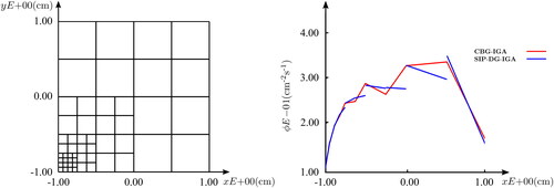
The performance of the SIP-DG discretization depends heavily upon the choice of penalty parameters; viz. they must be large enough to ensure definiteness and invertibility of the matrix equations, yet, not arbitrarily large that the iterative smoother is slow to converge. Excessive penalization at sharp boundary layers may even trigger the Gibbs phenomenon; i.e., the SIP-DG discretization tends to a CBG one as ${\mu }_f\to \infty$ (Hesthaven and Warburton 2010; Burman, Quarteroni, and Stamm 2010). Optimal rates of convergence in the $H^1$-norm and the $L_2$-norm have been proven for SIP-DG schemes for ${\mu }_f\propto \mathcal{O}(h^{-1})$ (Arnold 1982; Douglas and Dupont 1976). More rigorously, one follows the methodology of Shahbazi to establish a lower-bound of the penalty parameters via a coercivity analysis of the bilinear form (Shahbazi 2005).

Since the discretized system is only weakly coupled in energy, it is sufficient to consider separately the coercivity of each within-group bilinear form, the left-hand side of Equation 58(58) $$a_L^g({\widehat{\varphi }}^g,\widehat{w})+a_{\mathit{\text{IP}}}^g({\widehat{\varphi }}^g,\widehat{w})+a_{\mathit{\text{ext}}}^g({\widehat{\varphi }}^g,\widehat{w})=a_S^g(\widehat{\varphi },\widehat{w})+a_F^g(\widehat{\varphi },\widehat{w})+b^g(\widehat{w}),\hspace{1em}\forall \widehat{w}\in {\widehat{\mathcal{V}}}_{h,p}(\mathcal{T}).$$(58) or Equation 59(59) $$a_L^g({\widehat{\varphi }}^g,\widehat{w})+a_{\mathit{\text{IP}}}^g({\widehat{\varphi }}^g,\widehat{w})+a_{\mathit{\text{ext}}}^g({\widehat{\varphi }}^g,\widehat{w})=a_S^g(\widehat{\varphi },\widehat{w})+\frac{1}{{\mathrm{k}}_{\text{eff}}}{a}_F^g(\widehat{\varphi },\widehat{w}),\hspace{1em}\forall \widehat{w}\in {\widehat{\mathcal{V}}}_{h,p}(\mathcal{T}).$$(59) ; where $a_{\mathit{\text{lhs}}}^g$ is recalled below for some $\widehat{u}\in {\widehat{\mathcal{V}}}_{h,p}(\mathcal{T}),$ suppressing the spatial dependence for $g=1,\dots ,G:$ $$\begin{array}{cc}{a}_{\mathit{\text{lhs}}}^g(\widehat{u},\widehat{u})=a_L^g(\widehat{u},\widehat{u})+a_{\mathit{\text{IP}}}^g(\widehat{u},\widehat{u})+a_{\mathit{\text{ext}}}^g(\widehat{u},\widehat{u}),\hfill & \mathrm{\hspace{1em}(60}\mathrm{a)}\hfill \\ \begin{array}{cc}\hfill & =\sum _{V_e\in \mathcal{T}}{\int }_{V_e}\mathrm{}\mathrm{}{D}_e^g\overrightarrow{\nabla }\widehat{u}\mathrm{}\cdot \mathrm{}\overrightarrow{\nabla }\widehat{u}+{\Sigma }_{r,e}^g{(\widehat{u})}^2\mathit{\text{dV}}-\text{}\sum _{\partial V_f\in \partial V_{\mathit{\text{IP}}}}\text{}(1+\theta )\mathrm{}{\int }_{\partial V_f}\left[\right[\widehat{u}\left]\right]\left\{\right\{D^g\overrightarrow{\nabla }\widehat{u}\mathrm{}\cdot \mathrm{}\overrightarrow{n}\left\}\right\}\mathit{\text{dS}}\hfill \\ \hfill & +\sum _{\partial V_f\in \partial V_{\mathit{\text{IP}}}}{\mu }_f^g\int {}_{\partial V_f}{([\left[\widehat{u}\right]])}^2\mathit{\text{ dS}}+\sum _{\partial V_f\in \partial V_V}\frac{1}{2}{\int }_{\partial V_f}{(\widehat{u})}^2\mathit{\text{ dS}}.\hfill \end{array}\hfill & \mathrm{(60}\mathrm{b)}\hfill \end{array}$$

The within-group bilinear form is self-adjoint, $a_{\mathit{\text{lhs}}}^g=a_{\mathit{\text{lhs}}}^{g†},$ for $\theta =1;$ and since the discrete variational statements for both the primal problem, and the dual problem are formulated on the same mesh and their solutions sought in the same space, $\varphi ,{\varphi }^{†}\in {\widehat{\mathcal{V}}}_{h,p}(\mathcal{T}),$ the well-posedness of either depends upon a common coercivity analysis that yields a single set of energy-dependent penalty parameters.

Whilst the NIP-DG scheme is coercive for any ${\mu }_f>0,$ a lower-bound must be imposed for the IIP and the SIP variations. For reasons already discussed, only the latter is investigated; yet, for completeness, the variable θ is retained.

Sufficient penalization of each face $\partial V_f\in \partial V_{\mathit{\text{IP}}},$ should ensure the coercivity of the bilinear form with respect to the energy-norm, which is defined for some $\widehat{u}\in {\widehat{\mathcal{V}}}_{h,p}(\mathcal{T})$ and for $g=1,\dots ,G:$ (61) $$\Vert \widehat{u}{\Vert }_{{\widehat{ϵ}}^g}^2:=\sum _{V_e\in \mathcal{T}}{\int }_{V_e}{D}_e^g\overrightarrow{\nabla }\widehat{u}·\overrightarrow{\nabla }\widehat{u}+{\Sigma }_{r,e}^g{(\widehat{u})}^2\mathit{\text{ dV}}+\sum _{\partial V_f\in \partial V_{\mathit{\text{IP}}}}{\mu }_f^g{\int }_{\partial V_f}{([\left[\widehat{u}\right]])}^2\mathit{\text{ dS}}.$$(61)

Most popular in the literature are expressions of the general form: (62) $${\mu }_f=\rho \frac{\partial V_f}{V_e}\approx \frac{\rho }{h},\hspace{1em}\forall \partial V_f\in V_e\cap \partial V_{\mathit{\text{IP}}}\text{;}$$(62) whereby some large enough user-dependent parameter, $\rho ,$ is scaled by the mesh spacing, h; and quite often, only the largest value is retained.

More rigorously, Shahbazi establishes a lower-bound for the penalty parameters through a coercivity analysis of the bilinear form (Shahbazi 2005). Warburton and Hesthaven and separately Hillewaert adopted this same methodology and derived closed-form expressions for μ_f for particular straight-sided geometric primitives such as simplices; and quadrilaterals and hexahedra, respectively (Hesthaven and Warburton 2010; Hillewaert 2013). The work presented in this paper follows the developments of Owens et al.; and the penalty parameters are calculated via generalized eigenvalue problems, posed over the discontinuous faces, which are agnostic of the element type (Owens, Kópházi, and Eaton 2017).

One recalls Young’s inequality for the product of two scalars, $a$ and $b:$ (63) $$\mathit{\text{ab}}\le \frac{ϵa^2}{2}+\frac{b^2}{2ϵ},\hspace{1em}\forall ϵ>0.$$(63)

From the definition of jumps and averages, Equation 34a and Equation 34b, respectively, and then by letting $a=[[\widehat{u}]]$ and $b=\left\{\right\{D^g\overrightarrow{\nabla }\widehat{u}·\overrightarrow{n}\left\}\right\},$ the substitution of Equation 63(63) $$\mathit{\text{ab}}\le \frac{ϵa^2}{2}+\frac{b^2}{2ϵ},\hspace{1em}\forall ϵ>0.$$(63) into Equation 60b bounds the potentially negative term in the second line over all discontinuous faces, $\forall \partial V_f\in \partial V_{\mathit{\text{IP}}}.$ Collecting like-terms for $g=1,\dots ,G:$ (64) $$\begin{array}{cc}{a}_{\mathit{\text{lhs}}}^g(\widehat{u},\widehat{u})\hfill & \ge a_L^g(\widehat{u},\widehat{u})-\sum _{\partial V_f\in \partial V_{\mathit{\text{IP}}}}\frac{(1+\theta )}{2{ϵ}_f}{\int }_{\partial V_f}(\{\{D^g\overrightarrow{\nabla }\widehat{u}·\overrightarrow{n}\}\}{)}^2\mathit{\text{ dS}}\hfill \\ \hfill & +\sum _{\partial V_f\in \partial V_{\mathit{\text{IP}}}}({\mu }_f^g-\frac{(1+\theta ){ϵ}_f}{2}){\int }_{\partial V_f}{([\left[\widehat{u}\right]])}^2\mathit{\text{ dS}}+a_{\mathit{\text{ext}}}^g(\widehat{u},\widehat{u}).\hfill \end{array}$$(64)

By the definition in Equation 34b, the term ${(\{\left\{D^g\overrightarrow{\nabla }\widehat{u}\right\}\}·\overrightarrow{n})}^2$ is expanded out, to which Equation 63(63) $$\mathit{\text{ab}}\le \frac{ϵa^2}{2}+\frac{b^2}{2ϵ},\hspace{1em}\forall ϵ>0.$$(63) is applied with $ϵ=1;$ i.e., $a^2+b^2+2\mathit{\text{ab}}\le 2a^2+2b^2.$ The result is rewritten as a sum of integrals over patch boundaries, where individual terms are collected onto their respective patches; i.e.,: (65) $$\begin{array}{cc}{a}_{\mathit{\text{lhs}}}^g(\widehat{u},\widehat{u})\hfill & \ge a_L^g(\widehat{u},\widehat{u})-\sum _{V_e\in \mathcal{T}}(1+\theta )[\sum _{\partial V_f\in V_e\cap \partial V_{\mathit{\text{int}}}}\frac{{(D_e^g)}^2}{4{ϵ}_f}{\int }_{\partial V_f}{(\overrightarrow{\nabla }\widehat{u}·\overrightarrow{n})}^2\mathit{\text{ dS}}\hfill \\ \hfill & +\sum _{\partial V_f\in V_e\cap \partial V_D}\frac{{(D_e^g)}^2}{2{ϵ}_f}{\int }_{\partial V_f}{(\overrightarrow{\nabla }\widehat{u}·\overrightarrow{n})}^2\mathit{\text{ dS}}]\hfill \\ \hfill & +\sum _{\partial V_f\in \partial V_{\mathit{\text{IP}}}}({\mu }_f^g-\frac{(1+\theta ){ϵ}_f}{2}){\int }_{\partial V_f}{([\left[\widehat{u}\right]])}^2\mathit{\text{ dS}}+a_{\mathit{\text{ext}}}^g(\widehat{u},\widehat{u}).\hfill \end{array}$$(65)

Taking advantage of the equivalence of norms in the chosen function space, there exist discrete trace inequalities that bound from above integral quantities of the restriction of a function, or the normal component of its gradient, as defined over the boundary $\partial V_e;$ i.e., for some function $\widehat{u}\in {\widehat{\mathcal{V}}}_{h,p}(V_e):$ (66a) $$\Vert {\gamma }_0\widehat{u}{\Vert }_{L_2(\partial V_e)}^2\le C_{e,f}^0\Vert \widehat{u}{\Vert }_{L_2(V_e)}^2\text{;}$$(66a) (66b) $$\Vert {\gamma }_1\widehat{u}{\Vert }_{L_2(\partial V_e)}^2\le C_{e,f}^1\Vert \overrightarrow{\nabla }\widehat{u}{\Vert }_{L_2(V_e)}^2.$$(66b)

For i = 0, 1, $C_{e,f}^i$ are the trace inequality constants (TICs) that pertain to the Dirichlet and the Neumann traces in Equation 32a(32a) $${\gamma }_{0}u:=u{|}_{\partial V_e}\text{;}$$(32a) and Equation 32b(32b) $${\gamma }_{1}u:=\overrightarrow{\nabla }u·\overrightarrow{n}{|}_{\partial V_e}.$$(32b) , respectively. Those integrals over patch boundaries in Equation 65(65) $$\begin{array}{cc}{a}_{\mathit{\text{lhs}}}^g(\widehat{u},\widehat{u})\hfill & \ge a_L^g(\widehat{u},\widehat{u})-\sum _{V_e\in \mathcal{T}}(1+\theta )[\sum _{\partial V_f\in V_e\cap \partial V_{\mathit{\text{int}}}}\frac{{(D_e^g)}^2}{4{ϵ}_f}{\int }_{\partial V_f}{(\overrightarrow{\nabla }\widehat{u}·\overrightarrow{n})}^2\mathit{\text{ dS}}\hfill \\ \hfill & +\sum _{\partial V_f\in V_e\cap \partial V_D}\frac{{(D_e^g)}^2}{2{ϵ}_f}{\int }_{\partial V_f}{(\overrightarrow{\nabla }\widehat{u}·\overrightarrow{n})}^2\mathit{\text{ dS}}]\hfill \\ \hfill & +\sum _{\partial V_f\in \partial V_{\mathit{\text{IP}}}}({\mu }_f^g-\frac{(1+\theta ){ϵ}_f}{2}){\int }_{\partial V_f}{([\left[\widehat{u}\right]])}^2\mathit{\text{ dS}}+a_{\mathit{\text{ext}}}^g(\widehat{u},\widehat{u}).\hfill \end{array}$$(65) are substituted for Equation 66b(66b) $$\Vert {\gamma }_1\widehat{u}{\Vert }_{L_2(\partial V_e)}^2\le C_{e,f}^1\Vert \overrightarrow{\nabla }\widehat{u}{\Vert }_{L_2(V_e)}^2.$$(66b) ; and one seeks the sharpest TIC values to optimize the penalty parameters. Collecting like-terms and comparing against Equation 55(55) $$a(\widehat{u},\widehat{u})\ge C_{\beta }\Vert u{\Vert }_{\widehat{ϵ}}^2.$$(55) , the following must be satisfied for $g=1,\dots ,G:$ (67a) $$1-(1+\theta )[\sum _{\partial V_f\in V_e\cap \partial V_{\mathit{\text{int}}}}\frac{D_e^g{C}_{e,f}^1}{4{ϵ}_f}+\sum _{\partial V_f\in V_e\cap \partial V_D}\frac{D_e^g{C}_{e,f}^1}{2{ϵ}_f}]>0,\hspace{1em}\forall V_e\in {\mathcal{T}}^g(V)\text{;}$$(67a) (67b) $${\mu }_f^g-\frac{(1+\theta ){ϵ}_f}{2}>0,\hspace{1em}\forall \partial V_f\in \partial V_{\mathit{\text{IP}}}.$$(67b)

One must choose ${ϵ}_f>0,$ such that Equation 67a(67a) $$1-(1+\theta )[\sum _{\partial V_f\in V_e\cap \partial V_{\mathit{\text{int}}}}\frac{D_e^g{C}_{e,f}^1}{4{ϵ}_f}+\sum _{\partial V_f\in V_e\cap \partial V_D}\frac{D_e^g{C}_{e,f}^1}{2{ϵ}_f}]>0,\hspace{1em}\forall V_e\in {\mathcal{T}}^g(V)\text{;}$$(67a) is satisfied over each element. In anisotropic fashion, Drosson et al. achieved this by bounding from below each separate term in the sum over the F_e-number of faces of a given element (Drosson and Hillewaert 2013). Furthermore, the maximum necessary penalization is applied at a given interface to ensure that Equations 67(67a) $$1-(1+\theta )[\sum _{\partial V_f\in V_e\cap \partial V_{\mathit{\text{int}}}}\frac{D_e^g{C}_{e,f}^1}{4{ϵ}_f}+\sum _{\partial V_f\in V_e\cap \partial V_D}\frac{D_e^g{C}_{e,f}^1}{2{ϵ}_f}]>0,\hspace{1em}\forall V_e\in {\mathcal{T}}^g(V)\text{;}$$(67a) hold over every element that intersects at that interface. Encapsulated below, the penalty parameters can be calculated in a pre-processing step for $g=1,\dots ,G$ and $\forall \partial V_f\in \partial V_{\mathit{\text{IP}}}:$ (68a) $${\mu }_f^g>\{\begin{array}{cc}\frac{1}{8}{(1+\theta )}^2\underset{V_e\in \underset{e\prime }{\cap }{V}_{e\prime }\ni \partial V_f}{\mathrm{\text{max}}}{D}_e^g{C}_{e,f}^1{F}_e,\mathrm{\hspace{1em}}\mathrm{\hspace{1em}}\hfill & \partial V_f\in \partial V_{\mathit{\text{int}}}\text{;}\hfill \\ \frac{1}{4}{(1+\theta )}^2{D}_e^g{C}_{e,f}^1{N}_e,\mathrm{\hspace{1em}}\mathrm{\hspace{1em}}\hfill & \partial V_f\in \partial V_D.\hfill \end{array}$$(68a)

5.5. The trace inequality constants

In search of the smallest possible penalty parameters, a coercivity analysis has revealed the dependence on a constant, $C_{e,f}^1,$ from an inequality that bounds from above the Neumann trace of a function; q.v. Equation 66b(66b) $$\Vert {\gamma }_1\widehat{u}{\Vert }_{L_2(\partial V_e)}^2\le C_{e,f}^1\Vert \overrightarrow{\nabla }\widehat{u}{\Vert }_{L_2(V_e)}^2.$$(66b) . The μ_f are proportional to the corresponding TICs and thus, the problem of calculating optimized penalty parameters becomes one of minimizing these TICs (Owens, Kópházi, and Eaton 2017).

Warburton and Hesthaven provide closed-form expressions for the TICs of constant-Jacobian simplices (Warburton and Hesthaven 2003). Similarly, Hillewaert provides those for constant-Jacobian quadrilaterals and hexahedra (Hillewaert 2013): (69) $$C_{e,f}^{\mathit{\text{lit}}}={(p+1)}^2\frac{A(\partial V_f)}{V(V_e)}\text{;}$$(69) where p denotes the polynomial degree of the element; $A(\partial V_f)$ the area of $\partial V_f$ and $V(V_e)$ the volume of V_e. However, such expressions are derived from a different trace inequality, one that bounds the function itself and not its gradient. This may yield suitable penalty parameters for straight-sided linear finite elements; yet, they preclude any curved elements, or rather those that possesses a non-linear mapping; viz. NURBS-based IGA. For this reason, Owens et al. proposed a stiffness matrix-based approach, derived from the correct trace inequality, which numerically calculates provably sharp TICs for any general element face (Owens, Kópházi, Welch, et al. 2017).

First, the function in Equation 66b(66b) $$\Vert {\gamma }_1\widehat{u}{\Vert }_{L_2(\partial V_e)}^2\le C_{e,f}^1\Vert \overrightarrow{\nabla }\widehat{u}{\Vert }_{L_2(V_e)}^2.$$(66b) is expanded in a basis of NURBS basis functions, such that for $\widehat{u}\in {\widehat{\mathcal{V}}}_{h,p}(V_e):$ $$\overrightarrow{\nabla }\widehat{u}(\overrightarrow{r})=\sum _{i=1}^{N_e}{u}_i\overrightarrow{\nabla }{R}_i(\overrightarrow{r})=\underset{(1\times N_e)(N_e\times d)}{{\left[\underset{¯}{u}\right]}^T·\nabla \stackrel{R}{=},}\mathrm{\hspace{1em}}\mathrm{\hspace{1em}}\overrightarrow{r}\in V_e\text{;}$$ and similarly: $$\overrightarrow{\nabla }\widehat{u}(\overrightarrow{r})·\overrightarrow{n}(\overrightarrow{r})=\sum _{i=1}^{N_e}{u}_i\overrightarrow{\nabla }{R}_i(\overrightarrow{r})·\overrightarrow{n}(\overrightarrow{r})=\underset{(1\times N_e)(N_e\times d)(d\times 1)}{{\left[\underset{¯}{u}\right]}^T·\nabla \stackrel{R}{=}·\overrightarrow{n},}\mathrm{\hspace{1em}}\mathrm{\hspace{1em}}\overrightarrow{r}\in \partial V_f\text{;}$$ where $\underset{¯}{u}$ is the column vector of expansion coefficients and $\nabla \underset{=}{R}$ is a matrix that stores the gradient of each of the N_e-number of NURBS basis functions in each of the d-number of spatial directions as a separate column vector; i.e., ${(\nabla \underset{=}{R})}_{\mathit{\text{ij}}}=\partial R_i/\partial x_j\in {\mathbb{R}}^{N_e\times d}.$ Thus, Equation 66b(66b) $$\Vert {\gamma }_1\widehat{u}{\Vert }_{L_2(\partial V_e)}^2\le C_{e,f}^1\Vert \overrightarrow{\nabla }\widehat{u}{\Vert }_{L_2(V_e)}^2.$$(66b) can be rewritten in matrix notation: (70) $${\left[\underset{¯}{u}\right]}^T·{\underset{=}{S}}_{\partial V_f}·\underset{¯}{u}\le C_{e,f}^1{\left[\underset{¯}{u}\right]}^T·{\underset{=}{S}}_V·\underset{¯}{u}.$$(70)

The matrix ${\underset{=}{S}}_{\partial V_f}$ is constructed over a given face of a given patch and the matrix ${\underset{=}{S}}_{V_e}$ is constructed over the volume of that same patch. The entries of each are given below, respectively: (71a) $${({\underset{=}{S}}_{\partial V_f})}_{\mathit{\text{ij}}}=[{\int }_{\partial V_f}\overrightarrow{\nabla }{R}_i(\overrightarrow{r})·\overrightarrow{n}(\overrightarrow{r})\overrightarrow{\nabla }{R}_j(\overrightarrow{r})·\overrightarrow{n}(\overrightarrow{r})\mathit{\text{ dS}}]\in {\mathbb{R}}^{N_e\times N_e}\text{;}$$(71a) (71b) $${({\underset{=}{S}}_{V_e})}_{\mathit{\text{ij}}}=[{\int }_{V_e}\overrightarrow{\nabla }{R}_i(\overrightarrow{r})·\overrightarrow{\nabla }{R}_j(\overrightarrow{r})\mathit{\text{ dV}}]\in {\mathbb{R}}^{N_e\times N_e}.$$(71b)

Equation 70(70) $${\left[\underset{¯}{u}\right]}^T·{\underset{=}{S}}_{\partial V_f}·\underset{¯}{u}\le C_{e,f}^1{\left[\underset{¯}{u}\right]}^T·{\underset{=}{S}}_V·\underset{¯}{u}.$$(70) can be re-posed as a generalized eigenvalue problem that possesses N_e-number of discrete eigenvalues, ${\lambda }_i\ge 0$ for $i=1,\dots ,N_e:$ (72) $$\{\begin{array}{c}(\hspace{0.17em}{\underset{=}{S}}_{\partial V_f}-\lambda {\underset{=}{S}}_V)·\underset{¯}{x}=0,\hfill \\ \text{\hspace{0.5em}with\hspace{0.5em}}{\left[\underset{¯}{x}\right]}^T·{\underset{=}{S}}_V·\underset{¯}{x}=1.\hfill \end{array}$$(72)

One seeks the maximum eigenvalue, which corresponds to the provably sharp TIC in Equation 66b(66b) $$\Vert {\gamma }_1\widehat{u}{\Vert }_{L_2(\partial V_e)}^2\le C_{e,f}^1\Vert \overrightarrow{\nabla }\widehat{u}{\Vert }_{L_2(V_e)}^2.$$(66b) ; i.e., $C_{e,f}^1={\mathrm{\text{max}}}_i{\lambda }_i$ (Owens, Kópházi, and Eaton 2017). That being said, both of the matrices in the above are only symmetric positive semi-definite (SPSD) and do not form a regular pair. Accordingly, the generalized eigenvalue problem does not possess a spectrum of distinctly positive eigenvalues; and there exits a non-trivial intersection of the matrices’ null-spaces; i.e., $\text{null}(\hspace{0.17em}{\underset{=}{S}}_{\partial V_f})\cap \text{null}(\hspace{0.17em}{\underset{=}{S}}_{V_e})\ne \varnothing .$ Easily enough, this common null-space is identified as that 1D space spanned by the vector that represents the constant function, ${\underset{¯}{u}}_k,$ in ${\widehat{\mathcal{V}}}_{h,p}(V_e),$ which, as per the positivity of the right-hand side of Equation 66b(66b) $$\Vert {\gamma }_1\widehat{u}{\Vert }_{L_2(\partial V_e)}^2\le C_{e,f}^1\Vert \overrightarrow{\nabla }\widehat{u}{\Vert }_{L_2(V_e)}^2.$$(66b) , corresponds to the degenerate eigenvector associated with the single zero eigenvalue. Fortunately, the NURBS basis forms a partition of unity, such that the constant function is an $N_e$-dimensional vector of ones; i.e., ${\underset{¯}{u}}_k={[1,\dots ,1]}^T.$

It is possible to remove this singularity and compute the eigenvalues associated with the restriction of the pair of matrices to the complement of the null space (Saad 2011). Practically, this can be achieved via the (modified) Gram-Schmidt procedure. One forms an orthonormal set, $\underset{=}{Z},$ that spans the subspace of ${\mathbb{R}}^{N_e}$ by the orthogonal projection of some arbitrary input basis, $\underset{=}{U},$ which contains the constant function as the $k^{\mathit{\text{th}}}$ basis vector. Denoting $\underset{=}{Z}\prime$ as the orthogonal $(N_e\times N_e-1)$-matrix less the $k^{\mathit{\text{th}}}$ column, the transformation to the $(N_e-1)$-dimensional space ${\mathbb{R}}^{N_e}\backslash \text{span}{\underset{¯}{u}}_k$ is performed as: (73a) $${\underset{=}{S}}_{\partial V_{\mathit{f\prime }}}={[\underset{=}{Z}\prime ]}^T·{\underset{=}{S}}_{\partial V_f}·\underset{=}{\mathrm{Z\prime }}\text{;}$$(73a) (73b) $${\underset{=}{S}}_{V_{\mathit{e\prime }}}={[\underset{=}{Z}\prime ]}^T·{\underset{=}{S}}_{V_e}·\underset{=}{\mathrm{Z\prime }}\text{;}$$(73b) where the singularity has been orthogonalized out of the function space and the shared kernel removed such that the matrices ${\underset{=}{S}}_{\partial V_{\mathit{f\prime }}}$ and ${\underset{=}{S}}_{V_{\mathit{e\prime }}}$ are of one-less dimension than the originals. Although the former is still SPSD, the latter is now SPD and the LAPACK routine DSYGV can be employed to solve for the maximum eigenvalue by means of a Cholesky (LU) factorization (Anderson et al.. 1999). Importantly, the positive eigenvalues of the original generalized eigenvalue problem are preserved; the new pair of matrices is equivalent to the original pair (Saad 2011). In the interest of a wholly-local AMR strategy, an explicit orthogonalization of the matrices in Equation 73(73a) $${\underset{=}{S}}_{\partial V_{\mathit{f\prime }}}={[\underset{=}{Z}\prime ]}^T·{\underset{=}{S}}_{\partial V_f}·\underset{=}{\mathrm{Z\prime }}\text{;}$$(73a) is not expected to be computationally expensive since an h-refinement forms new discontinuous patches. Consequently, the dimensions of any matrices in Equations 71(71a) $${({\underset{=}{S}}_{\partial V_f})}_{\mathit{\text{ij}}}=[{\int }_{\partial V_f}\overrightarrow{\nabla }{R}_i(\overrightarrow{r})·\overrightarrow{n}(\overrightarrow{r})\overrightarrow{\nabla }{R}_j(\overrightarrow{r})·\overrightarrow{n}(\overrightarrow{r})\mathit{\text{ dS}}]\in {\mathbb{R}}^{N_e\times N_e}\text{;}$$(71a) remains relatively small; i.e.,, $N_e\sim \mathcal{O}({10}^1).$

For the example of a 2D unit pin-cell mesh, a geometry that is ubiquitous in reactor physics, one compares the different TICs obtained from Equation 66a(66a) $$\Vert {\gamma }_0\widehat{u}{\Vert }_{L_2(\partial V_e)}^2\le C_{e,f}^0\Vert \widehat{u}{\Vert }_{L_2(V_e)}^2\text{;}$$(66a) and Equation 66b(66b) $$\Vert {\gamma }_1\widehat{u}{\Vert }_{L_2(\partial V_e)}^2\le C_{e,f}^1\Vert \overrightarrow{\nabla }\widehat{u}{\Vert }_{L_2(V_e)}^2.$$(66b) ; v. Figure 5. The $C_{e,f}^0$ are calculated using a mass matrix approach; viz. substitution of the stiffness matrices in Equation 72(72) $$\{\begin{array}{c}(\hspace{0.17em}{\underset{=}{S}}_{\partial V_f}-\lambda {\underset{=}{S}}_V)·\underset{¯}{x}=0,\hfill \\ \text{\hspace{0.5em}with\hspace{0.5em}}{\left[\underset{¯}{x}\right]}^T·{\underset{=}{S}}_V·\underset{¯}{x}=1.\hfill \end{array}$$(72) for mass matrices, which do not need to be orthogonalized. The parametric study of TIC values is inspired by that of Owens et al.; however, theirs did not allow for a fair comparison since it was performed over a mesh of degenerate NURBS patches (Owens, Kópházi, and Eaton 2017). As per the stiffness matrix approach, the derivatives of the volumetric NURBS basis functions must be square-integrable at the boundary and thus, the patch must be non-degenerate. Otherwise, $C_{e,f}^1$ are arbitrarily large, and increasingly so, for an increasingly large quadrature set; q.v. Section 2.1. For this reason, the authors concluded that the penalty parameters for the faces of the elements of a pin-cell mesh may be underestimated by as much as $\times 50$ when employing the literature expressions, Equation 69(69) $$C_{e,f}^{\mathit{\text{lit}}}={(p+1)}^2\frac{A(\partial V_f)}{V(V_e)}\text{;}$$(69) , or the mass matrix method to calculate the TICs.

Figure 5. For the example of a 2D unit pin-cell mesh of 13 non-degenerate bi-quadratic NURBS patches (left), a comparison is made between those TICs, $C_{e,f}^{\mathit{\text{lit}}},C_{e,f}^0$ and $C_{e,f}^1,$ as calculated from the literature, Equation 69(69) $$C_{e,f}^{\mathit{\text{lit}}}={(p+1)}^2\frac{A(\partial V_f)}{V(V_e)}\text{;}$$(69) , the mass matrix method, Equation 66a(66a) $$\Vert {\gamma }_0\widehat{u}{\Vert }_{L_2(\partial V_e)}^2\le C_{e,f}^0\Vert \widehat{u}{\Vert }_{L_2(V_e)}^2\text{;}$$(66a) , and the stiffness matrix method, Equation 66b(66b) $$\Vert {\gamma }_1\widehat{u}{\Vert }_{L_2(\partial V_e)}^2\le C_{e,f}^1\Vert \overrightarrow{\nabla }\widehat{u}{\Vert }_{L_2(V_e)}^2.$$(66b) , respectively. The ten distinct faces are labeled 1 through 10; and all TIC values are normalized by $\times V(V_e)/A\partial V_f.$ The distinction between Faces $\partial V_{7a}$ and $\partial V_{7b}$ is such that the former is the the single distinct face of the central (red) circle constructed from a single degenerate NURBS patch; whereas the latter belongs to the set of distinct faces that belong to the central circle as it is presented, constructed from five non-degenerate NURBS patches. Those TIC values that are invariant with any change to the radii are presented in the table (right). (V. the web-based version for reference to color.).

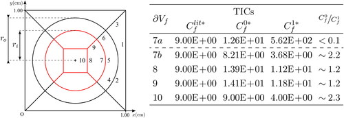
The geometry for the current analysis is constructed from 13 bi-quadratic non-degenerate NURBS patches; v. Figure 7. The central fuel pin is represented by a circle, constructed from five patches; the cladding is represented by an annulus, constructed from four patches; and so is the surrounding moderator region. Taking into account all lines of symmetry, there are only four distinct element types and only ten distinct faces, labeled 1 through 10, need to be considered. For each distinct face, $C_{e,f}^0$ and $C_{e,f}^1$ are computed. To facilitate a further comparison with those TICs, $C_{e,f}^{\mathit{\text{lit}}},$ taken from the literature, Equation 69(69) $$C_{e,f}^{\mathit{\text{lit}}}={(p+1)}^2\frac{A(\partial V_f)}{V(V_e)}\text{;}$$(69) , all TIC values are normalized by $\times V(V_e)/A(\partial V_f).$ Numerical integration is performed consistently with a Legendre-Gauss quadrature set of N_q = 10, in each parametric direction over each element.

The moderator region is defined uniquely by the outer-radius, which is varied between 0.05 and 0.45 cm. The results for Faces $\partial V_1,\partial V_2$ and $\partial V_3$ are presented in the top left, the top right and the middle left, respectively, of Figure 6. The shape of the annular region is defined by the ratio of the radii; and therefore, the inner-radius was fixed at 0.025 cm and the outer-radius was varied between 0.05 and 0.45 cm. The results for Faces $\partial V_4,\partial V_5$ and $\partial V_6$ are presented in the middle right, the bottom left and the bottom right, respectively, of Figure 6. The shape of the central pin, as represented by five non-degenerate patches, is defined by the inner-radius, which is varied between 0.05 and 0.45 cm. However, the normalized TICs are invariant with r_i and these results for Faces $\partial V_{7b},\partial V_8,\partial V_9$ and $\partial V_{10}$ are presented in the table in Figure 5.

Figure 6. A parametric study that compares TIC values for the distinct Faces $\partial V_1$ (top left), $\partial V_2$ (top right), $\partial V_3$ (middle left), $\partial V_4$ (middle right), $\partial V_5$ (bottom left), and $\partial V_6$ (bottom right) of a 2D unit pin-cell mesh as the outer-radius is varied; v. Figure 5. In each instance, the volume patch and the face patches may be defined by $r_o,$ which is varied between 0.05 and 0.45 cm. In the case of $\partial V_4,\partial V_5$ and $\partial V_6,r_i$ is fixed at 0.025 cm. (V. the web-based version for reference to color.).

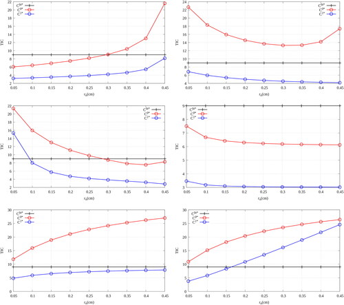
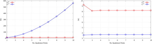
For completeness, a comparison is included for those TICs evaluated over the surface of degenerate NURBS patch; viz. the central pin is constructed instead from a single degenerate NURBS patch. The distinction between Faces $\partial V_{7a}$ and $\partial V_{7b}$ is such that the former is the the single distinct face of the central (red) circle constructed from a single degenerate patch; whereas the latter belongs to the set of distinct faces that belong to the central circle constructed from five non-degenerate patches. Similarly, those TIC over Face $\partial V_{7a}$ are invariant with $r_i;$ and one observes that $C_{7a}^0<0.01\times C_{7a}^1.$ However, this is clearly dependent upon the size of the numerical quadrature set; v. Figure 7.

Figure 7. A parametric study that compares TICs for the distinct Faces $\partial V_{7a}$ (left) and $\partial V_{7b}$ (right) of a 2D unit pin-cell mesh as the number of quadrature points is varied; v. Figure 5. In each instance, the TICs are invariant with any change to the radii. (V. the web-based version for reference to color.).

In the consideration of constant-Jacobian elements, both the literature method and the mass matrix method yield the same result; or rather, an overestimation of the required TIC value. In the consideration of non-constant-Jacobian elements, again, the mass matrix method yields TIC values larger than those of the stiffness matrix method. This was also generally true of the literature method, with the exception of Face $\partial V_6$ for an increasingly large outer-radius. Whilst the mass matrix method for evaluating TIC values has not been investigated further, one is confident that the stiffness matrix method allows for sharper bounds on the resulting penalty parameters because information has not been discarded and the gradient of the function has been taken into account. Moreover, the proposed approach is robust in its application to any element type.

5.6. Optimized penalty parameters

For completeness, the effect of varying the penalty parameters for an SIP-DG-IGA discretization of the 1G NDE is studied for the example of a 2D unit homogeneous pin-cell with reflective BCs; qq.v. Table 1 and Section 6.1.2. The μ_f from Equation 68(68a) $${\mu }_f^g>\{\begin{array}{cc}\frac{1}{8}{(1+\theta )}^2\underset{V_e\in \underset{e\prime }{\cap }{V}_{e\prime }\ni \partial V_f}{\mathrm{\text{max}}}{D}_e^g{C}_{e,f}^1{F}_e,\mathrm{\hspace{1em}}\mathrm{\hspace{1em}}\hfill & \partial V_f\in \partial V_{\mathit{\text{int}}}\text{;}\hfill \\ \frac{1}{4}{(1+\theta )}^2{D}_e^g{C}_{e,f}^1{N}_e,\mathrm{\hspace{1em}}\mathrm{\hspace{1em}}\hfill & \partial V_f\in \partial V_D.\hfill \end{array}$$(68a) for each face are varied as ${\mu }_f^{*}=\alpha \times {\mu }_f,$ for $\alpha =[0,10];$ and the effect on the discretization error and the conditioning of the system is presented in Figure 8 for p = 2, 3, 4. For each dataset, the mesh is $9\times \mathit{\text{KI}}$-h-refined uniformly. The same conditioning effects were observed for the study of $9\times \mathit{\text{KI}}$-1-refinement. However, the discretization error was less sensitive to any variation in μ_f because of the higher-order continuity in the basis.

Figure 8. A parametric study of the $H^1$-error (right) and the spectral conditioning (right) of the SIP-DG-IGA discretization of the 1G NDE for the example of a 2D unit pin-cell mesh; qq.v. Table 1 and Section 6.1.2. The penalty parameters of each face are varied as ${\mu }_f^{*}=\alpha \times {\mu }_f.$ (V. the web-based version for reference to color.).

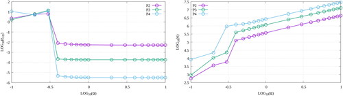
Table 1. The nuclear data for the 2D 1G MMS verification.

Material	g	D^g(cm)	${\Sigma }_t^g$ (^−1)	${\Sigma }_{s0}^{g\to 1}$ (cm ^−1)
(1)	1	$3.333\mathrm{E}-01$	$1.000\mathrm{E}+00$	$5.000\mathrm{E}-01$

The effect of under-penalization is apparent in Figure 8 by the poor values of the $H^1$-error. Although not obvious from the scale, the error attains a minimum for the choice of ${\mu }_f^{*}={\mu }_f$ and thereafter plateaus for $\alpha >1;$ viz. there is no gain in accuracy for super-penalization. Another obvious effect is that on the conditioning, $\kappa (\underset{=}{A}),$ of the discretized system; viz. the matrix becomes increasingly ill-conditioned for increasingly large μ_f. Taking $\kappa (\underset{=}{A})$ as the ratio of the largest to the smallest eigenvalues of $\underset{=}{A},$ the spectral condition number is used to gauge the number of iterations that are required to solve the matrix equation. The eigenvalues are computed using the PETSc GMRes solver with the flag -ksp_monitor_singular_value (Balay et al. 2018). Rather than absolute values, one is more interested in the general trends that varying μ_f has on the conditioning of the system. Whilst the approximation of the largest singular value is often fairly accurate, that of the smallest is only typically so upon convergence; and thus, restarts are avoided by setting the restart parameter to 10, 000.

The effect of the polynomial degree is also noticeable in Figure 8; that is, improved accuracy can be attained, for the same number of elements, for bases constructed from increasingly higher-order polynomials. This only has implications for the asymptotic convergence ranges and assumes that the analysis is performed over a sufficiently graded mesh, which suggests an instability in a basis of higher-order polynomials over a coarse mesh (Gahalaut, Kraus, and Tomar 2013). Furthermore, the discrete system becomes increasingly more dense as the polynomial degree of the basis increases; and thus, it becomes increasingly more expensive to smoothen.

At the time of writing, only standard preconditioners and algebraic multi-grid methods were considered. However, the authors are aware of research into subspace correction preconditioners for DG discretizations of elliptic problems using a basis of Gauss-Lobatto functions (Pazner and Kolev 2022). This would allow for (S)IP schemes using arbitrarily large penalty parameters and polynomial degrees to be solved efficiently (Pazner and Kolev 2022). Subsequent research should investigate whether such preconditioners are also effective for higher-order NURBS-based discretizations.

6. The numerical results

This section presents some numerical results for the AMR-h(p) strategies developed in Section 2.2 and Section 3. Unless otherwise stated, all operations are performed to optimize the discretization error in the $H^1$-(semi)norm. The AMR strategies are compared against uniform refinement for a series of verification test cases using the method of manufactured solutions (MMS); and a couple of reactor physics benchmarks. Any data-plots that make reference to the DoFs of the discretized system justly account for all unknowns that were solved for in the complete system.

The SIP-DG-IGA spatial discretization schemes developed here have been implemented in a new, modern Fortran code (Metcalf, Reid, and Cohen 2011). Adopting a distributed memory computing architecture, one makes use of the Open MPI message passing library; as well as the PETSc library and its capacity for parallelization of its sparse linear solvers and its compressed row storage (CRS) data structures for large sparse matrices (Balay et al. 2018). All jobs are submitted to the general purpose Imperial College London (ICL) HPC cluster computing service (CX1). The within-group matrix equations are converged to machine precision using PETSc’s conjugate gradient smoother, pre-conditioned by the BoomerAMG algebraic multi-grid method from the HYPRE library (Henson and Yang 2002). The scalar neutron flux is converged to a tolerance of $1.00\mathrm{E}-06$ between successive source iterations; and the eigenvalue is converged to a tolerance of $1.00\mathrm{E}-08$ between successive power iterations. An arbitrary upper-limit of ten is imposed upon the polynomial degree of the NURBS basis over the coarser current mesh; and therefore p_max = 11 over the reference mesh.

The number of outer-iterations required to attain convergence is reduced by bootstrapping the reference solution from the previous AMR-iteration, using it as an initial guess over the reference mesh in the current i^th-iteration (Wang 2009).

6.1. The method of manufactured solutions (MMS) verification

The method of manufactured solutions (MMS) is used to investigate the spatial discretizations of the multi-group NDE; cf. an overview by Salari et al. (Salari and Knupp 2000). A smooth manufactured solution is chosen to test against theoretical orders of accuracy (Rivière 2008; Warsa 2008): (74a) $$|e{|}_{H^1}\le C_1{h}^{\mathrm{\text{min}}\{p,r\}}\text{;}$$(74a) (74b) $$\Vert e{\Vert }_{L_2}\le C_2{h}^{\mathrm{\text{min}}\{p+1,r\}}\text{;}$$(74b) where $e=\varphi -\widehat{\varphi }$ is the discretization error; h is the characteristic mesh-spacing, p is the polynomial degree of the underlying NURBS basis; r denotes the regularity index of the true solution; and $C_1$ and $C_2$ are constants independent of h and p. As per the tensor-product structure of the NURBS basis, Equations 3(3) $$R_{i,j}^{p,q}(\xi ,\eta )=\frac{N_i^p(\xi )M_j^q(\eta )W_{i,j}}{\sum _{i\prime =1}^N\sum _{j\prime =1}^M{N}_{i\prime }^p(\xi )M_{j\prime }^q(\eta )W_{i\prime ,j\prime }}.$$(3) , the polynomial degree in the inequalities above, Equations 74(74a) $$|e{|}_{H^1}\le C_1{h}^{\mathrm{\text{min}}\{p,r\}}\text{;}$$(74a) , is actually $p={\mathrm{\text{min}}}_i\left\{p_i\right\}$ for $i=\xi ,\eta .$

For some manufactured solution, ${\varphi }^g,$ the (semi-)analytical manufactured fixed-source, $q_x^g,$ can be evaluated for $g=1,\dots ,G:$ (75) $$q_x^g=(L^g-S^g)\varphi .$$(75)

First, the manufactured solution and source are used to study the convergence rates of the uniform refinement of a Cartesian mesh; and then of a more challenging pin-cell mesh. Second, one studies the NRG-AMR-h(p) strategy to verify all mesh-to-mesh interpolation procedures and the capacity to enforce continuity over irregular meshes that contain hanging-nodes.

6.1.1. MMS verification: a Cartesian mesh

The first MMS verification case consists of a Cartesian mesh mesh defined over $V={[0,1]}^2.$ It comprises a homogeneous material whose properties are prescribed in Table 1. The coarsest mesh is composed of four equal-volume squares represented by bilinear NURBS patches. Assuming a one-speed, or one-group (1G), energy approximation, the manufactured solution is chosen as a standing wave equation: $$\{\begin{array}{cc}{\varphi }^n(\overrightarrow{r})=\hspace{0.17em}\mathrm{\text{cos}}\hspace{0.17em}(B_x^{n}x)\hspace{0.17em}\mathrm{\text{cos}}\hspace{0.17em}(B_y^{n}y),\mathrm{\hspace{1em}}\mathrm{\hspace{1em}}\hfill & \overrightarrow{r}\in V\text{;}\mathrm{(}\text{76a}\mathrm{)}\hfill \\ B_x^n,B_y^n:=(2n+1)\pi ,\hspace{1em}\hfill & \forall n\ge 0\text{;}\mathrm{(}\text{76b}\mathrm{)}\hfill \end{array}$$ where ${\varphi }^n$ denotes an odd harmonic mode as characterized by the geometric buckling, $B_x^n$ and $B_y^n.$ To allow for the maximum attainable convergence rates, the manufactured solution has been chosen to be smooth; yet, it cannot be represented exactly by arbitrarily high-order NURBS bases. Moreover, the homogeneous Neumann (reflective) BC is naturally satisfied.

6.1.1.1. Uniform refinement

For the KI-refinement of linear, quadratic and cubic B-splines, the $H^1$-errors for the SIP-DG-IGA spatial discretization are presented in Figure 9 for the manufactured solution chosen as the first, third and fifth harmonics of the standing wave equation; q.v. Equation 76. Qualitatively similar plots were obtained for the $L_2$-error; however, for brevity, these have not been presented. Under refinement, the discontinuous discretization schemes converge to the analytical solution; and asymptotically, they attain their theoretical orders of accuracy, as presented in Table 2.

Figure 9. The convergence plots, ${ϵ}_{H^1}$v h (left) and ${ϵ}_{H^1}$v DoFs (right), for the MMS verification of the uniform refinement of the SIP-DG-IGA 1G NDE over a 2D Cartesian mesh. The manufactured solution is chosen as per Equation 76 for n = 0 (top row), n = 1 (middle row) and n = 2 (bottom row). (V. the web-based version for reference to color.).

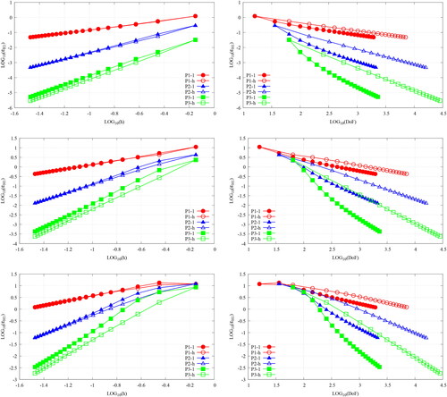
Table 2. The asymptotic orders of accuracy, Equations 74, for the MMS verification of the uniform refinement of the SIP-DG-IGA 1G NDE over a 2D Cartesian mesh.

		KI-1		KI-h
	p	${ϵ}_{H^1}$	${ϵ}_{L_2}$	${ϵ}_{H^1}$	${ϵ}_{L_2}$
(n = 0)	1	1.00	2.00	1.00	2.00
	2	2.05	3.03	2.00	2.99
	3	2.98	3.98	3.00	4.00
(n = 1)	1	1.00	2.01	1.02	1.98
	2	2.06	3.05	2.00	3.00
	3	3.01	4.03	3.00	3.99
(n = 2)	1	1.00	2.01	1.04	1.96
	2	2.08	3.09	2.01	3.01
	3	3.06	4.09	3.01	3.98

The convergence rates are evaluated as the slope of the last few points from each dataset.

Whilst the mesh spacing, h, does give some insight into how the discretization error varies under refinement, it does not reveal the true computational effort required; viz. the number of elements in the mesh does not vary under DE-refinement. Therefore, one should also consider the DoFs of the discrete system; this is a better metric by which to compare non-uniform refinement strategies. Yet, the DoFs may still not reflect the true computational effort since one must also take into consideration the calculation of the TICs. One notes that it becomes increasingly more expensive to solve the orthogonalized eigenvalue problem for a patch with an increasingly large internal refinement structure; q.v. Section 5.2.

For such a homogeneous problem with a smooth underlying solution, exploiting higher-order continuity in the basis yields more accuracy per DoF than that compared to a similar h-refinement. Moreover, one remarks that h-refinement becomes increasingly more expensive for increasingly large polynomial degrees.

An expected observation is that of the prolonged pre-asymptotic range of convergence, which can be seen on the left-hand side of Figure 9; it becomes increasingly large for increasingly-more oscillatory solutions. For Galerkin-based methods, unique solvability exists for certain conditions imposed upon the choice the discrete approximation space; viz. the minimum resolution for asymptotic convergence (Melenk, Parsania, and Sauter 2013).

6.1.1.2. Adaptive local refinement

The results of the NRG-AMR-h(p) strategy for chasing the global $H^1$-error in the SIP-DG-IGA spatial discretization are presented in Figure 10 for the manufactured solution chosen as the first, third and fifth harmonics of the standing wave equation; q.v. Equation 76. These results are compared against those obtained for uniform h-refinement. For a coarsest mesh of linear B-splines, the NRG-AMR-hp strategy, denoted in the legend by P1-NRG-hp, exhibits exponential rates of convergence. Such a homogeneous and smooth problem favors p-refinement until p_max of the basis is attained, after which, only h-refinement is available. For coarsest meshes of linear and quadratic B-splines, the NRG-AMR-h strategy, denoted in the legend by P1-NRG-h and P2-NRG-h, respectively, yields algebraic rates of convergence, which are comparable with those of uniform refinement. One recalls that the computation is actually performed on the reference mesh, which is more refined than the current coarser mesh by one-level of uniform hp-refinement.

Figure 10. The convergence plots, ${ϵ}_{H^1}$v DoFs, for the MMS verification of the NRG-AMR-h(p) of the SIP-DG-IGA 1G NDE over a 2D Cartesian mesh. The manufactured solution is chosen as per Equation 76 for n = 0 (top left), n = 1 (top right) and n = 2 (bottom). (V. the web-based version for reference to color.).

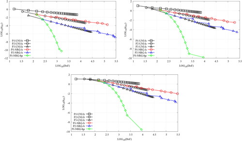
Inevitably, enforcing continuity over irregular meshes does introduce some errors since a more-refined subspace is penalized against a less-refined neighbor. Accordingly, it may appear that the local-refinement strategy does not offer much of a competitive edge for such a simple problem. However, these results do verify consistency in all mechanisms of the AMR strategy.

6.1.2. MMS verification: a pin-cell mesh

The second MMS verification case consists of a more-challenging pin-cell mesh defined over $V={[0,1]}^2.$ It comprises a homogeneous material whose properties are prescribed in Table 3. The coarsest mesh is composed of nine equal-volume non-degenerate bi-quadratic NURBS patches. Assuming a two-group (2G) energy approximation, the manufactured solution is chosen as: $$\{\begin{array}{cc}{\varphi }^g(\overrightarrow{r})=\hspace{0.17em}\mathrm{\text{sin}}\hspace{0.17em}(B_x^{g}x)\hspace{0.17em}\mathrm{\text{sin}}\hspace{0.17em}(B_y^{g}y),\mathrm{\hspace{1em}}\mathrm{\hspace{1em}}\hfill & \overrightarrow{r}\in V\text{;}\mathrm{(}\text{77a}\mathrm{)}\hfill \\ B_x^g,B_y^g:=(2g+1)\pi ,\mathrm{\hspace{1em}}\mathrm{\hspace{1em}}\hfill & \text{for\hspace{0.5em}}g=1,2\text{;}\mathrm{(}\text{77b}\mathrm{)}\hfill \end{array}$$ where ${\varphi }^g$ denotes an odd harmonic mode as characterized by the geometric buckling, $B_x^g$ and $B_y^g.$ Again, the manufactured solution has been chosen to be infinitely differentiable. However, now, the homogeneous Dirichlet (zero-flux) BC is naturally satisfied.

Table 3. The nuclear data for the 2D 2G MMS verification.

Material	g	D^g (cm)	${\Sigma }_t^g$ (cm ^−1)	${\Sigma }_{s0}^{g\to 1}$ (cm^−1)	${\Sigma }_s^{g\to 2}$ (cm^−1)
(1) -	1	3.333E − 01	1.000E − 01	5.000E − 01	2.500E − 01
(1) -	2	3.333E − 01	1.000E − 01	0.000E − 01	5.000E − 01

6.1.2.1. Uniform refinement

For the KI-refinement of quadratic, cubic and quartic NURBS bases, the $H^1$-errors for the SIP-DG-IGA spatial discretization are presented in Figure 11 for the multi-group components of the manufactured solution chosen as the third and fifth harmonics of the standing wave equation; q.v. Equation 77. Qualitatively similar plots were obtained for the $L_2$-error; however, for brevity, these have not been presented. Under refinement, the discontinuous discretization schemes converge to the analytical solution; and asymptotically, they attain their theoretical orders of accuracy for KI-h-refinement, as presented in Table 4. However, for KI-1-refinement, one remarks a degree of super-convergence, which may be explained either by the higher-order continuity in the basis or the weak imposition of the Dirichlet BCs. Although not presented in this paper, for the same pin-cell mesh with naturally enforced reflective BCs and manufactured solutions chosen as per Equation 76, one observed the expected theoretical rates of convergence.

Figure 11. The convergence plots, ${ϵ}_{H^1}$v h (left) and ${ϵ}_{H^1}$v DoFs (right), for the MMS verification of the uniform refinement of the SIP-DG-IGA 2G NDE over a 2D pin-cell mesh. The manufactured solutions are chosen as per Equation 77 for g = 1, 2. (V. the web-based version for reference to color.).

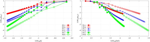
Table 4. The asymptotic orders of accuracy, Equations 74, for the MMS verification of the uniform refinement of the SIP-DG-IGA 2G NDE over a 2D pin-cell mesh.

	KI-1		KI-h
P	${ϵ}_{H^1}$	${ϵ}_{L_2}$	${ϵ}_{H^1}$	${ϵ}_{L_2}$
2	2.06	3.15	2.00	3.03
3	3.09	4.18	3.00	3.97
4	4.29	5.40	3.99	5.02

The convergence rates are evaluated as the slope of the last few points from each dataset.

6.1.2.2. Adaptive local refinement

The results of the NRG-AMR-h(p) strategy for chasing the global $H^1$-error in the SIP-DG-IGA discretization are presented in Figure 12 for the multi-group components of the manufactured solution chosen as the third and fifth harmonics of the standing wave equation; q.v. Equation 77. These results are compared against those obtained for uniform h-refinement. For a coarsest mesh of quadratic NURBS basis functions, the NRG-AMR-hp strategy, denoted in the legend by P2-NRG-hp, again, exhibits faster rates of convergence; although this time the mesh iteration is not dominated by p-refinements. For coarsest meshes of quadratic and cubic NURBS basis functions, the NRG-AMR-h strategy, denoted in the legend by P2-NRG-h and P3-NRG-h, respectively, again, yields algebraic rates of convergence that are comparable with those of uniform refinement.

Figure 12. The convergence plots, ${ϵ}_{H^1}$v DoFs, for the MMS verification of the NRG-AMR-h(p) of the SIP-DG-IGA 2G NDE over a 2D pin-cell mesh. The prefixes M1- and M2- denote the use of energy-independent and energy-dependent meshes, respectively. The manufactured solutions are chosen as per Equation 77 for g = 1, 2. (V. the web-based version for reference to color.).

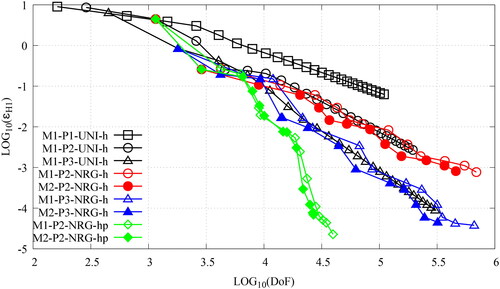
Within a multi-group formalism, it is fitting to test the capacity for energy-dependent meshes, denoted in the legend by the prefix M2-, which yield more accuracy per DoF when compared to the refinement strategies that employ energy-independent meshes, denoted in the legend by the prefix M1-. The use of interpolation-based error measures can be measured against the (reciprocal) effectivity index, ${\theta }_{H^1};$ this is presented in Figure 13 (Bangerth and Rannacher 2003). Since ${\theta }_{H^1}$ tends to values slightly larger than unity, one can approximate the remaining error in the discretization, which may be used to terminate the mesh iteration procedure (Wilson, Eaton, and Kópházi 2024).

Figure 13. The plots of the effectivity index, ${\theta }_{H^1}$v DoFs, for the MMS verification of the NRG-AMR-h(p) of the SIP-DG-IGA 2G NDE over a 2D pin-cell mesh. The prefixes M1- and M2- denote the use of energy-independent and energy-dependent meshes, respectively. The manufactured solutions are chosen as per Equation 77 for g = 1, 2. (V. the web-based version for reference to color.).

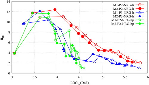
Again, the results do verify consistency in the mechanisms of the AMR strategy over irregular meshes for rational geometries.

6.2. The 2D IAEA/ANL BSS-11 (LWR) benchmark

The 2D IAEA benchmark for the 2G NDE is the BSS-11 quarter-core LWR problem taken from the Argonne National Laboratory (ANL) Benchmark Problem Book, Supplement 2 (Argonne National Laboratory 1977). Taken at the mid-plane, $z=1.90\mathrm{E}+02$ cm, this 2D benchmark is adapted from the full 3D (xyz) one (Theler 2013). Complete specifications for this benchmark, including geometry and nuclear data, are provided by Wilson et al. (Wilson, Eaton, and Kópházi 2024).

The coarsest Cartesian mesh is constructed from 241 bilinear NURBS patches. A reference solution is provided by Wilson et al.; viz. ${\mathrm{k}}_{\text{eff}}=1.0295886369,$ which is in good agreement with the literature (Wilson, Eaton, and Kópházi 2024; Argonne National Laboratory 1977). The spatial distribution of the multi-group components of both the scalar neutron flux and the scalar neutron importance are presented in Figure 14, for the QoI chosen as the ${\mathrm{k}}_{\text{eff}}.$

Figure 14. The spatial distributions of the multi-group components of the scalar neutron flux (left) and the scalar neutron importance (right) of the 2G NDE for the 2D IAEA/ANL BSS-11 benchmark. The QoI is the ${\mathrm{k}}_{\text{eff}}.$ (V. the web-based version for reference to color.).

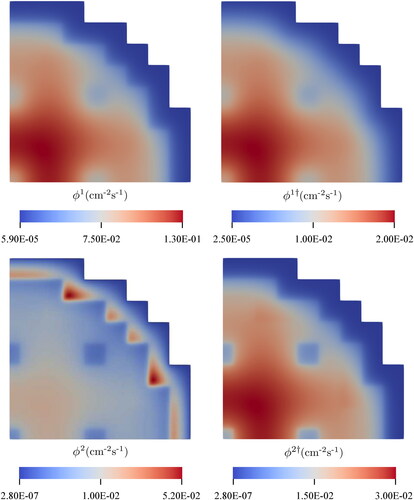
Those meshes generated after the $9^{\mathit{\text{th}}}$ AMR-iteration of the AMR-h and AMR-hp strategies are presented in Figures 15 and 16, respectively. One notes that within the same AMR-h(p) framework, Wilson et al. obtained qualitatively similar meshes for a constraint-based continuous Bubnov-Galerkin (CBG-)IGA spatial discretization of the multi-group NDE (Wilson, Eaton, and Kópházi 2024).

Figure 15. The energy-independent meshes (top) and the energy-dependent meshes (middle and bottom) generated at the $9^{\mathit{\text{th}}}$ AMR-iteration of the NRG-AMR-h (left) and the DWR-AMR-h (right) of the SIP-DG-IGA 2G NDE for the 2D IAEA/ANL BSS-11 benchmark. The QoI is the ${\mathrm{k}}_{\text{eff}}.$ (V. the web-based version for reference to color.).

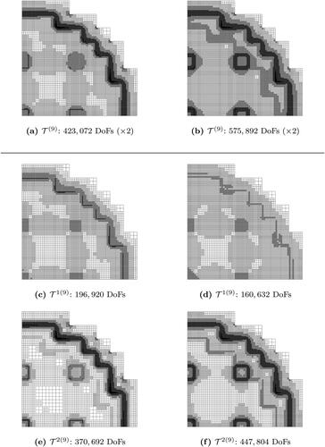
Figure 16. The energy-independent meshes (top) and the energy-dependent meshes (middle and bottom) generated at the $9^{\mathit{\text{th}}}$ AMR-iteration of the NRG-AMR-hp (left) and the DWR-AMR-hp (right) of the SIP-DG-IGA 2G NDE for the 2D IAEA/ANL BSS-11 benchmark. The QoI is the ${\mathrm{k}}_{\text{eff}}.$ (V. the web-based version for reference to color.).

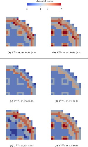
At the cost of an increasingly ill-conditioned matrices, the hp-refinement strategies performed better than the corresponding h-refinement ones; v. Figure 17. The computation times for the former were not prohibitive since the chosen algebraic multi-grid pre-conditioner worked effectively.

Figure 17. The convergence plots, ϵ_QoI v DoFs, for the uniform refinement (black), the NRG-AMR (red) and the DWR-AMR (blue) of the SIP-DG-IGA 2G NDE for the 2D IAEA/ANL BSS-11 benchmark. The prefixes M1- and M2- denote the use of energy-independent and energy-dependent meshes, respectively. The QoI is the ${\mathrm{k}}_{\text{eff}}.$ (V. the web-based version for reference to color.).

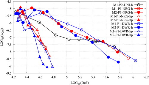
Both AMR strategies performed better than the uniform one. This is unsurprising as the ${\mathrm{k}}_{\text{eff}}$ is a global quantity and both AMR strategies chase the global error in the primal solution. However, at the cost of solving the dual problem, the DWR-AMR strategies do allow for a better allocation of resources; and better still when employing energy-dependent meshes.

6.3. The 2D BIBLIS (PWR) benchmark

The checkerboard fuel-loading pattern of the 2D BIBLIS benchmark for the 2G NDE better represents the core of an operating PWR. First proposed by Finemann and Wagner, Herbert provided an updated version to correspond to a rods-out configuration (Hébert,1985 2019). Complete specifications for this benchmark, including geometry and nuclear data, are provided by Wilson et al. (Wilson, Eaton, and Kópházi 2024).

The coarsest Cartesian mesh is constructed from 257 bilinear NURBS patches. The spatial distribution of the multi-group components of both the scalar neutron flux and the scalar neutron importance are presented in Figure 18. From the literature, ${\mathrm{k}}_{\text{eff}}=1.0250103$ (Hébert 2019). However, in this instance, the QoI is chosen as the absorption in Material 5; and again, a reference is provided by Wilson et al. (Wilson, Eaton, and Kópházi 2024).

Figure 18. The spatial distributions of the multi-group components of the scalar neutron flux (left) and the scalar neutron importance (right) for the 2G NDE for the 2D BIBLIS benchmark. The QoI is the absorption in Material 5. (V. the web-based version for reference to color.).

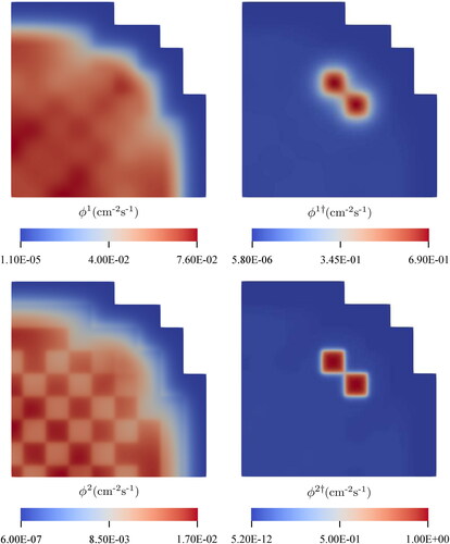
The meshes generated after the $9^{\mathit{\text{th}}}$ AMR-iteration of the AMR-h and AMR-hp strategies are presented in Figures 19 and 20, respectively. Again, within the same AMR-h(p) framework, Wilson et al. obtained qualitatively similar meshes for their constraint-based CBG-IGA spatial discretization of the multi-group NDE (Wilson, Eaton, and Kópházi 2024).

Figure 19. The energy-independent meshes (top) and the energy-dependent meshes (middle and bottom) generated at the $9^{\mathit{\text{th}}}$ AMR-iteration of the NRG-AMR-h (left) and the DWR-AMR-h (right) of the SIP-DG-IGA 2G NDE for the 2D BIBLIS benchmark. The QoI is the absorption in Material 5. (V. the web-based version for reference to color.).

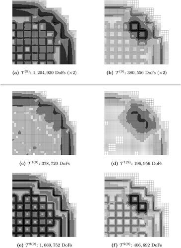
Figure 20. The energy-independent meshes (top) and the energy-dependent meshes (middle and bottom) generated at the $9^{\mathit{\text{th}}}$ AMR-iteration of the NRG-AMR-hp (left) and the DWR-AMR-hp (right) of the SIP-DG-IGA 2G NDE for the 2D BIBLIS benchmark. The QoI is the absorption in Material 5. (V. the web-based version for reference to color.).

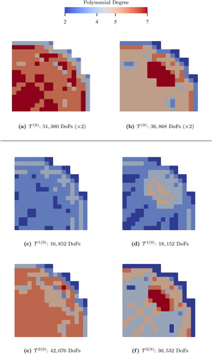
Indicative timings for the different stages of analysis at the $9^{\mathit{\text{th}}}$ AMR-iteration are presented in Table 5. In any case, the relative time spent in the Assembly stage is negligible. However, the relative time spent in the Refinement stage became dominating for the AMR-h strategies, which includes the calculating of the interpolation-based error measures; and calculating the TICs for the optimized penalty parameters over each surface of the more-refined reference meshes. Whereas the relative time spent in the Solutions tage became dominating for the AMR-hp strategies, which includes evaluating the group-to-group sources over energy-dependent meshes.

Table 5. The indicative timings for the different stages of analysis at the 9^th AMR-iteration of the NRG-AMR-h(p) and DWR-AMR-h(p) of the SIP-DG-IGA 2G NDE over energy-dependent meshes for the 2D BIBLIS benchmark.

Stage	NRG-AMR-h	NRG-AMR-hp	DWR-AMR-h	DWR-AMR-hp
Assembly	<1%	5%	1%	5%
Solution	6%	60%	11%	61%
Refinement	94%	35%	88%	34%
Total (s)	198	10	85	7

The Solution stage includes: evaluating the group-to-group sources over energy-dependent meshes. The Refinement stage includes: calculating the a posteriori interpolation-based error measures; and calculating the TICs for the optimized penalty parameters over the more-refined reference meshes.

Indeed, the DWR-AMR strategies consistently and reliably reduce the error in the QoI at each subsequent AMR-iteration; v. Figure 21. Moreover, the overall performance of the SIP-DG-IGA discretization benefits from DWR-AMR strategies, specifically with regard to h-refinement for localized QoIs, because the computational effort is focused about the region(s) of interest; i.e., Material 5. By contrast, the NRG-AMR-h strategy saw an explosion of elements throughout the computational domain and thus, there were many more faces over which to calculate the TICs; cf. Figure 19c and e vs Figure 19d and f. As a result, the NRG-AMR-h strategy took twice as long as the DWR-AMR-h strategy to complete the $9^{\mathit{\text{th}}}$ AMR-iteration. Again, at the cost of solving the dual problem, the DWR-AMR-hp strategy took less time than the NRG-AMR-hp strategy to complete the $9^{\mathit{\text{th}}}$ AMR-iteration. Moreover, the DWR-AMR strategies for the proposed SIP-DG-IGA discretization took less time than for the aforementioned constraint-based CBG-IGA discretization to complete the $9^{\mathit{\text{th}}}$ AMR-iteration over similar energy-independent meshes (Wilson, Eaton, and Kópházi 2024). This implies that more time was spent establishing the constraint-based equations over the irregular meshes than calculating the TICs over all element faces.

Figure 21. The convergence plots, ϵ_QoI v DoFs, for the uniform refinement (black) and the NRG-AMR (red) and the DWR-AMR (blue) of the SIP-DG-IGA 2G NDE for the 2D BIBLIS benchmark. The prefixes M1- and M2- denote the use of energy-independent and energy-dependent meshes, respectively. The QoI is the absorption in Material 5. (V. the web-based version for reference to color.).

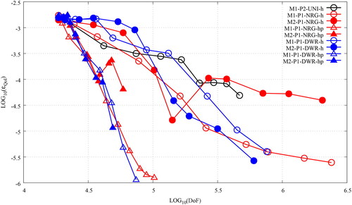
7. Conclusion

This paper proposes self-adaptive NRG-AMR-h(p) and DWR-AMR-h(p) strategies for a SIP-DG-IGA spatial discretization of the multi-group NDE, which can be readily extended to full 3D heterogeneous nuclear reactor physics problems. Optimized penalty parameters, based upon a rigorous coercivity analysis, were derived for general element types to ensure sufficient, not excessive, penalization of the discrete solution field across the spatial mesh(es). The spatial discretization results in large, sparse, SPD matrices that can benefit from PETSc’s capacity for distributed-memory CRS data structures; and the parallel implementation of its PCG smoothers. Moreover, the algebraic multi-grid pre-conditioner was effective for those problems posed over Cartesian meshes.

For global quantities such as the ${\mathrm{k}}_{\text{eff}},$ the NRG-AMR strategies for were competitive with the DWR-AMR ones. However, for localized QoI, the former tended to become less performant than uniform h-refinement; and especially so for the use of energy-dependent meshes, since certain multi-group components were left under-resolved. Conversely, the DWR-AMR strategies consistently and reliably reduced the error in the QoI at each subsequent AMR-iteration.

Although not presented in this paper, the AMR-h(p) algorithms for the proposed SIP-DG-IGA multi-group NDE did generate qualitatively similar meshes to those generated by a continuous Bubnov-Galerkin (CBG-)IGA spatial discretization that enforces continuity in the solution field across irregular patch interfaces via constraint equations based upon a master-slave relationship and the conservative interpolation between surface meshes (Wilson, Eaton, and Kópházi 2024). Despite incurring at least twice as many DoFs as the latter over qualitatively similar meshes, the former offers a more-compact stencil and more flexibility in terms of local refinement.

It is difficult to compare directly the efficiencies of the proposed AMR strategies over different continuous and discontinuous spatial discretization schemes over qualitatively similar meshes. Indeed, the computational effort and time spent in the Refinement stage of the proposed SIP-DG-IGA spatial discretization does increase sharply with the number elements because the TICs must be calculated over all element faces; cf. Table 5. Nevertheless, it was observed, in some instances, that more time can be spent establishing the constraint-based equations over irregular interfaces (Wilson, Eaton, and Kópházi 2024).

Acknowledgement

The authors thank the high-performance computing (HPC) service support team at Imperial College London.

Disclosure statement

No potential conflict of interest was reported by the author(s).

Data statement

In accordance with EPSRC funding requirements, all supporting data used to create figures in this paper may be accessed via the following URL: https://doi.org/10.5281/zenodo.10370345.

Additional information

Funding

S. G. Wilson acknowledges the financial support of the Engineering and Physical Sciences Research Council (EPSRC) under their doctoral training partnership (DTP) scheme (EPSRC Grant No. EP/N509486/1). S. G. Wilson also acknowledges the financial support of Rolls-Royce for the funding of the CASE conversion of the EPSRC DTP PhD

References

- Alvarez, G. B., A. F. D. Loula, E. G. D. do Carmo, and F. A. Rochinha. 2006. A discontinuous finite element formulation for Helmholtz equation. Comput. Methods Appl. Mech. Eng. 195 (33–36):4018–35. 10.1016/j.cma.2005.07.013.
- Anderson, E., Z. Bai, C. Bischof, S. Blackford, J. Demmel, J. Dongarra, J. Du Croz, et al. 1999. LAPACK users’ guide. Technical Report, Society for Industrial and Applied Mathematics.
- Argonne National Laboratory. 1977. Argonne Code Center: Benchmark problem book. Report No. ANL-7416, Argonne National Laboratory.
- Arnold, D. N. 1982. An interior penalty finite element method with discontinuous elements. SIAM J. Numer. Anal. 19 (4):742–60. 10.1137/0719052.
- Arnold, D. N., F. Brezzi, B. Cockburn, and L. D. Marini. 2002. Unified analysis of discontinuous Galerkin methods for elliptic problems. SIAM J. Numer. Anal. 39 (5):1749–79. 10.1137/S0036142901384162.
- Balay, S., S. Abhyankar, M. Adams, J. Brown, P. Brune, K. Buschelman, L. Dalcin, et al. 2018. PETSc users manual: Revision 3.9. Report No. ANL-95/11 Rev. 3.9, Argonne National Laboratory.
- Bangerth, W., and R. Rannacher. 2003. Adaptive finite element methods for differential equations. In Lectures in mathematics ETH Zurich. Springer. doi: 10.1007/978-3-0348-7605-6.
- Beer, G. 2015. Advanced numerical simulation methods: From CAD data directly to simulation results. Taylor & Francis Group, CRC Press.
- Boltzmann, L. E. 1872. Weitere Studien über das Wärmegleichgewicht unter Gasmolekülen. Sitzungsberichte Der Mathematisch-Naturwissenschaftlichen Classe Der Kaiserlichen Akademie Der Wissenschaften 66:275–370. 10.1007/978-3-322-84986-1_3.
- Brezzi, F., B. Cockburn, L. D. Marini, and E. Süli. 2006. Stabilization mechanisms in discontinuous Galerkin finite element methods. Computer Methods in Applied Mechanics and Engineering 195 (25–28):3293–310. 10.1016/j.cma.2005.06.015.
- Brunero, F. 2012. Discontinuous Galerkin methods for isogeometric analysis. Master’s thesis, Università degli Studi di Milano. https://www.gs.jku.at/pubs/2012brunero-dipl.pdf.
- Burman, E., A. Quarteroni, and B. Stamm. 2010. Interior penalty continuous and discontinuous finite element approximations of hyperbolic equations. J. Sci. Comput. 43 (3):293–312. 10.1007/s10915-008-9232-6.
- Castillo, P. 2002. Performance of discontinuous Galerkin methods for elliptic PDEs. SIAM J. Sci. Comput. 24 (2):524–47. 10.1137/S106482750138833. 10.1137/S1064827501388339
- Cottrell, J. A., T. J. R. Hughes, and Y. Bazilevs. 2009. Isogeometric analysis: Toward integration of CAD and FEA. John Wiley & Sons, Inc.
- Cottrell, J., T. Hughes, and A. Reali. 2007. Studies of refinement and continuity in isogeometric structural analysis. Comput. Methods Appl. Mech. Eng. 196 (41–44):4160–83. 10.1016/j.cma.2007.04.007.
- Cox, M. G. 1972. The numerical evaluations of B-splines. IMA J. Appl. Math. 10 (2):134–49. 10.1093/imamat/10.2.134.
- de Boor, C. 1972. On calculating with B-splines. Journal of Approximation Theory 6 (1):50–62. 10.1016/0021-9045.(72)90080-9. 10.1016/0021-9045(72)90080-9
- Demkowicz, L. 2004. Projection based interpolation. Report No. ICES 04-03, University of Texas at Austin.
- Demkowicz, L. 2007. Computing with hp-adaptive finite elements: One and two dimensional elliptic and Maxwell problems. Vol. 1 of Chapman & Hall/CRC applied mathematics and nonlinear science series. Chapman & Hall/CRC. doi: 10.1201/9781420011685.
- Di Pietro, D. A. and A. Ern. 2012. Mathematical aspects of discontinuous Galerkin methods. Vol. 69 of Mathémathiques et applications. Springer. doi: 10.1007/978-3-642-22980-0.
- Douglas, J., Jr, and T. Dupont. 1976. Interior penalty procedures for elliptic and parabolic Galerkin methods. Vol. 58 of Lecture notes in physics. Springer-Verlag. doi: 10.1007/BFb0120591.
- Drosson, M., and K. Hillewaert. 2013. On the stability of the symmetric interior penalty method for the Spalart-Allmaras turbulence model. J. Comput. Appl. Math. 246:122–35. 10.1016/j.cam.2012.09.019.
- Dryja, M. 2003. On discontinuous Galerkin methods for elliptic problems with discontinuous coefficients. Comput. Methods Appl. Math. 3 (1):76–85. 10.2478/cmam-2003-0007.
- Epshteyn, Y., and B. Rivière. 2007. Estimation of penalty parameters for symmetric penalty Galerkin methods. J. Comput. Appl. Math. 206 (2):843–72. 10.1016/j.cam.2006.08.029.
- Ern, A., and J.-L. Guermond. 2004. Theory and practice of finite elements. Vol. 159 of Applied mathematical sciences. Springer. doi: 10.1007/978-1-4757-4355-5.
- Farrell, P. E., and J. R. Maddison. 2011. Conservative interpolation between volume meshes by local Galerkin projection. Comput. Methods Appl. Mech. Eng. 200 (1–4):89–100. 10.1016/j.cma.2010.07.015.
- Gahalaut, K. P. S., J. K. Kraus, and S. K. Tomar. 2013. Multigrid methods for isogeometric discretisation. Comput. Methods Appl. Mech. Eng. 253 (100):413–25. 10.1016/j.cma.2012.08.015.
- Grote, M. J., A. Schneebeli, and D. Schötzau. 2007. Interior penalty discontinuous Galerkin method for Maxwell’s equations: Energy norm error estimates. J. Comput. Appl. Math. 204 (2):375–86. 10.1016/j.cam.2006.01.044
- Hébert, A. 1985. Application of the Hermite method for finite element reactor calculations. Nucl. Sci. Eng. 91 (1):34–58. 10.13182/NSE85-A17127.
- Hébert, A. 2019. A user guide for Trivac version-4 . Report No. IGE-293 , Ecole Polytechnique de Montréal - Institut de Génie Nucléaire .
- Hébert, A. 2020. Applied reactor physics. 3rd ed. Presses Internationales Polytechnique.
- Henson, V. E., and U. M. Yang. 2002. BoomerAMG: A Parallel algebraic multigrid solver and preconditioner. Appl. Numer. Math. 41 (1):155–77. 10.1016/S0168-9274.(01)00115-5. 10.1016/S0168-9274(01)00115-5
- Hesthaven, J. S., and T. Warburton. 2010. Nodal discontinuous Galerkin methods: Algorithms. Analysis and applications. Vol. 54 of Texts in applied mathematics. Springer. doi: 10.1007/978-0-387-72067-8.
- Hillewaert, K. 2013. Development of the discontinuous Galerkin method for high-resolution, large-scale CFD and acoustics in industrial geometries. PhD thesis, Université Catholique de Louvain. https://hdl.handle.net/2078.1/pul:29303100319670.
- Kaplan, S. 1969. Variational methods in nuclear engineering. Adv. Nucl. Sci. Technol. 3 (135):185–221. 10.1016/B978-0-12-029305-6.50010-8.
- Lewis, E. E., and W. F. Miller, Jr. 1984. Computational methods of neutron transport. John Wiley & Sons, Inc.
- Li, B. Q. 2006. Discontinuous finite elements in fluid dynamics and heat transfer. Computational fluid and solid mechanics. Springer. doi: 10.1007/1-84628-205-5.
- Melenk, J. M., A. Parsania, and S. Sauter. 2013. General DG-methods for highly indefinite Helmholtz problems. J. Sci. Comput. 57 (3):536–81. 10.1007/s10915-013-9726-8.
- Metcalf, M., J. Reid, and M. Cohen. 2011. Modern Fortran explained. Numerical mathematics and scientific computation. Oxford University Press. doi: 10.1093/oso/9780198811893.001.0001.
- Nitsche, J. A. 1971. Über ein Variationsprinzip zur Lösung von Dirichlet-Problemen bei Verwendung von Teilrämen, die keinen Randbedingungen unterworfen sind. Vol. 36 of Abhandlungen aus dem mathematischen Seminar der Universität Hamburg. Springer. 10.1007/BF02995904
- Oden, J. T., I. Babuŝka, and C. E. Baumann. 1998. A discontinuous hp finite element method for diffusion problems. Comput. Phys. 146 (2):491–519. 10.1006/jcph.1998.6032.
- Oden, J. T., and J. N. Reddy. 2011. An introduction to the mathematical theory of finite elements. Dover Publications. doi: 10.1002/nme.1620110715.
- Owens, A. R., J. Kópházi, and M. D. Eaton. 2017b. Optimal trace inequality constants for interior penalty discontinuous Galerkin discretisations of elliptic operators using arbitrary elements with non-constant Jacobians. Comput. Phys. 350:847–70. 10.1016/j.jcp.2017.09.020.
- Owens, A. R., J. Kópházi, J. A. Welch, and M. D. Eaton. 2017a. Energy dependent mesh adaptivity of discontinuous isogeometric discrete ordinate methods with dual weighted residual error estimators. Comput. Phys. 335:352–86. 10.1016/j.jcp.2017.01.035.
- Owens, A. R. 2017. Discontinuous isogeometric analysis methods for the first-order form of the neutron transport equation with discrete oridnate angular discretisation. PhD thesis, Imperial College London.
- Pazner, W., and T. Kolev. 2022. Uniform subspace correction preconditioners for discontinuous Galerkin methods with h(p)-refinement. Commun. Appl. Math. Comput. 4 (2):697–727. 10.1007/s42967-021-00136-3.
- Percell, P., and M. F. Wheeler. 1978. A local residual finite element procedure for elliptic equations. SIAM J. Numer. Anal. 15 (4):705–14. 10.1137/0715047.
- Piegl, L., and W. Tiller. 1997. The NURBS book: Monographs in visual communication. Springer.
- Rivière, B. 2008. Discontinuous Galerkin methods for solving elliptic and parabolic equations: Theory and Implementation. Frontiers in Applied Mathematics. SIAM. doi: 10.1137/1.9780898717440.
- Saad, Y. 2011. Numerical methods for large eigenvalue problems. 2nd ed., Classics in Applied Mathematics. SIAM. doi: 10.1137/1.9781611970739.
- Salari, K., and P. Knupp. 2000. Code verification by the method of manufactured solutions . Report No. SAND2000-1444. Sandia National Laboratories.
- Sangalli, G., and M. Tani. 2016. Isogeometric preconditioners based on fast solvers for the Sylvester equation. SIAM J. Sci. Comput. 38 (6):A3644–A3671. 10.1137/16M1062788.
- Schunert, S., Y. Wang, R. Martineau, and M. D. DeHart. 2015. A new mathematical adjoint for the modified SAAF-SN equations. Ann. Nucl. Energy 75:340–52. 10.1016/j.anucene.2014.08.028.
- Shahbazi, K. 2005. An explicit expression for the penalty parameter of the interior penalty method. Comput. Phys. 205 (2):401–7. 10.1016/j.jcp.2004.11.017.
- Theler, G. 2013. Unstructured grids and the multigroup neutron diffusion equation. Sci. Technol. Nucl. Install. 2013:1–26. 10.1155/2013/641863.
- Wang, Y., W. Bangerth, and J. Ragusa. 2009. Three-dimensional h-adaptivity for the multigroup neutron diffusion equations. Prog. Nucl. Energy 51 (3):543–55. 10.1016/j.pnucene.2008.11.005.
- Wang, Y. 2009. Adaptive mesh refinement solution techniques for the multigroup SN transport equation using a higher-order discontinuous finite element method. PhD thesis, Texas A&M University. https://hdl.handle.net/1969.1/ETD-TAMU-2009-05-641.
- Warburton, T., and J. S. Hesthaven. 2003. On the constants in hp-finite element trace inverse inequalities. Comput. Methods Appl. Mech. Eng. 192 (25):2765–73. 10.1016/S0045-7825.(03)00294-9. 10.1016/S0045-7825(03)00294-9
- Warsa, J. S. 2008. A continuous finite element-based, discontinuous finite element method for S N transport. Nucl. Sci. Eng. 160 (3):385–400. 10.13182/NSE160-385TN.
- Wheeler, M. F. 1978. An elliptic collocation-finite element method with interior penalties. SIAM J. Numer. Anal. 15 (1):152–61. 10.1137/0715010.
- Wilson, S. G., M. D. Eaton, and J. Kópházi. 2024. Energy-dependent, self-adaptive mesh h(p)-refinement of a constraint-based continuous Bubnov-Galerkin isogeometric analysis spatial discretization of the multi-group neutron diffusion equations with dual-weighted residual error measures. Journal of Computational and Theoretical Transport 53:1–64. 10.1080/23324309.2024.2313460.
- Wilson, S. G., J. Kópházi, A. R. Owens, and M. D. Eaton. 2018. Interior penalty schemes for discontinuous isogeometric methods with an application to nuclear reactor physics. In Proc. of the International Conference of Nuclear Engineering (ICONE26), Vol. 3: Nuclear Fuel and Material, Reactor Physics and Transport Theory . ASME. 10.1115/ICONE26-81322
- Wilson, S. G. 2021. Self-adaptive isogeometric spatial discretisations of the first and second-order forms of the neutron transport equation with dual-weighted residual error measures and diffusion acceleration. PhD thesis, Imperial College London.