Multidimensional soliton systems

ABSTRACT

This concise review aims to provide a summary of the most relevant recent experimental and theoretical results for solitons, i.e. self-trapped bound states of nonlinear waves, in two- and three-dimensional (2D and 3D) media. In comparison with commonly known one-dimensional solitons, which are, normally, stable modes, a challenging problem is the propensity of 2D and 3D solitons to instability, caused by the occurrence of the critical or supercritical wave collapse (catastrophic self-compression) in the same spatial dimensions. A remarkable feature of multidimensional solitons is their ability to carry vorticity; however, 2D vortex rings and 3D vortex tori are subject to a strong splitting instability. Therefore, it is natural to categorize the basic results according to physically relevant settings which make it possible to stabilize fundamental (non-topological) and vortex solitons against the collapse and splitting, respectively. The present review is focused on schemes that were recently elaborated in terms of Bose-Einstein condensates and similar photonic setups. These are two-component systems with spin-orbit coupling, and ones stabilized by the beyond-mean-field Lee-Huang-Yang effect. The latter setting has been implemented experimentally, giving rise to stable self-trapped quasi-2D and 3D quantum droplets. Characteristic examples of stable three-dimensional solitons: a semi-vortex (top) and mixed-mode (bottom) modes in the binary Bose-Einstein condensate, stabilized by the spin-orbit coupling.

KEYWORDS:

• Bose-Einstein condensates
• nonlinear optics
• vortices
• stability
• spin-orbit coupling
• quantum droplets

1. Introduction: multidimensional solitons and their proneness to instabilities

The absolute majority of theoretical and experimental work which has been performed for solitons, i.e. self-trapped solitary waves in nonlinear systems, deal with one-dimensional (1D) settings. Extension of the soliton concepts to multidimensional spaces is a very promising but also challenging direction. A fascinating possibility is to create new species of solitary states in two- and three-dimensional (2D and 3D) geometries with intrinsic topological structures. An obvious option is to create 2D and 3D vortex solitons carrying an intrinsic angular momentum, which may be considered as a classical counterpart of the spin of quantum particles. Multi-component solitons can be used to build more sophisticated topological structures, such as skyrmions, hopfions (alias twisted vortex tori in the 3D space), monopoles, knots, and others [1–5].

However, the work with 2D and 3D solitons encounters fundamental difficulties. First, unlike the fundamental 1D models that give rise to solitons, such as the Korteweg – de Vries, sine-Gordon, and nonlinear Schrödinger (NLS) equations, in most cases multidimensional equations are not integrable (there are some integrable 2D models – most notably, the Kadomtsev-Petviashvili equations [6]). The lack of the integrability of basic 2D and 3D soliton equations may be considered as a technical difficulty, because relevant solutions, once they are not available in an exact form, can be constructed by means of approximate analytical methods, such as the variational approximation (VA), and the availability of powerful computers makes it possible to produce numerical solutions in all relevant cases. However, in 2D and 3D settings self-attractive nonlinearities, which are necessary for the formation of solitons, give rise to a fundamental problem, viz., instability of the localized states, due to the fact that the same settings give rise to the wave collapse (alias blowup, i.e. catastrophic self-compression of the wave field leading to the formation of a true singularity after a finite evolution time), which is illustrated by Figure 1(a) [8–11].

Figure 1. (a) Onset of the critical collapse featured by the unstable evolution of a TS (Townes soliton), as produced by simulations of the 2D version of Equation (1)(1) $i{\psi }_t+\frac{1}{2}{\mathrm{\nabla }}^2\psi +|\psi {|}^{\sigma -1}\psi =0.$(1) with $\sigma =3$, shown in the radial cross-section. (b) An example of the splitting instability of a 3D soliton with embedded vorticity S = 2 (a vortex torus). The left and right panels display surfaces $\left|u(x,y,\tau ,z)\right|=\text{const}$, which are produced, respectively, as a stationary solution of the 3D counterpart of Equation (26)(26) $i{u}_z+\frac{1}{2}(u_{xx}+u_{\tau \tau })+|u{|}^{2}u-|u{|}^{4}u=0.$(26) (the input for simulations of the full equation), and as a result of the simulated evolution. The figures are borrowed from book [7].

The instability problem is exhibited by the general model based on the NLS equation in the space of dimension D with the self-attractive nonlinear term of power σ [the Kerr nonlinearity in optics [12] and collisional nonlinearity in Bose-Einstein condensates (BECs) [13] correspond to σ = 3]:

(1) $i{\psi }_t+\frac{1}{2}{\mathrm{\nabla }}^2\psi +|\psi {|}^{\sigma -1}\psi =0.$(1)

Complex field ψ in Equation (1)(1) $i{\psi }_t+\frac{1}{2}{\mathrm{\nabla }}^2\psi +|\psi {|}^{\sigma -1}\psi =0.$(1) represents the local amplitude of electromagnetic waves in optics, or the wave function of matter waves in BEC, considered in the mean-field (MF) approximation. Solutions of Equation (1)(1) $i{\psi }_t+\frac{1}{2}{\mathrm{\nabla }}^2\psi +|\psi {|}^{\sigma -1}\psi =0.$(1) are characterized by the dynamical invariants, viz., the norm

(2) $N=\int {\left|\psi (x,y,z)\right|}^2{d}^{D}x,$(2)

and Hamiltonian,

(3) $H=\int (\frac{1}{2}|\mathrm{\nabla }\psi {|}^2-\frac{2}{\sigma +1}|\psi {|}^{\sigma +1})d^{D}x\equiv H_{\mathrm{grad}}+H_{\mathrm{self}-\mathrm{focusing}},$(3)

where the integration is performed over the D-dimensional space with coordinates $\{x_1,\dots ,x_D\}$.

In addition to that, moving and vortical solutions are characterized, respectively, by the additional dynamical invariants, viz., the vectorial linear momentum, $\mathbf{P}=-i\int {\psi }^{\ast }\mathrm{\nabla }\psi d^{D}x$, and angular momentum,

(4) $\mathbf{M}=-i\int {\psi }^{\ast }(\mathbf{r}\times \mathrm{\nabla })\psi d^{D}x,$(4)

where $\ast$ stands for the complex conjugate. In the 2D space with coordinates $(x,y)$, vector (4(4) $\mathbf{M}=-i\int {\psi }^{\ast }(\mathbf{r}\times \mathrm{\nabla })\psi d^{D}x,$(4) ) has the single component,

(5) $M_z=i\int {\psi }^{\ast }(y\frac{\partial \psi }{\partial x}-x\frac{\partial \psi }{\partial y})d^{D}x.$(5)

Note that, while expressions (4(4) $\mathbf{M}=-i\int {\psi }^{\ast }(\mathbf{r}\times \mathrm{\nabla })\psi d^{D}x,$(4) ) and (5(5) $M_z=i\int {\psi }^{\ast }(y\frac{\partial \psi }{\partial x}-x\frac{\partial \psi }{\partial y})d^{D}x.$(5) ) seem complex, the application of the integration by parts demonstrates that their values are actually real for localized states (solitons, in particular).

In optics, the spatiotemporal propagation of light in media with anomalous group-velocity dispersion (GVD) is governed by the NLS Equation (1)(1) $i{\psi }_t+\frac{1}{2}{\mathrm{\nabla }}^2\psi +|\psi {|}^{\sigma -1}\psi =0.$(1) , in which time t is replaced by the propagation distance, z, while the temporal variable,

(6) $\tau \equiv t-z/V_{\mathrm{gr}},$(6)

where $V_{\mathrm{gr}}$ is the group velocity of the carrier wave [12], plays the role of an additional coordinate. Spatiotemporal solitons predicted by such a model are often called light bullets (LBs) [14].

Stationary solutions to Equation (1)(1) $i{\psi }_t+\frac{1}{2}{\mathrm{\nabla }}^2\psi +|\psi {|}^{\sigma -1}\psi =0.$(1) are looked for as

(7) $\psi (x_1,\mathrm{\nabla },x_D;t)=e^{-i\mu t}\varphi (x_1,\mathrm{\nabla },x_D),$(7)

where real constant µ is called the chemical potential in the context of matter waves in BEC [13], and stationary wave function ϕ is determined by equation

(8) $\mu \varphi +\frac{1}{2}{\mathrm{\nabla }}^2\varphi +|\varphi {|}^{\sigma -1}\varphi =0$(8)

(localized solutions of Equation (8)(8) $\mu \varphi +\frac{1}{2}{\mathrm{\nabla }}^2\varphi +|\varphi {|}^{\sigma -1}\varphi =0$(8) may only correspond to µ < 0).

To explain the onset of the collapse in the framework of Equation (1)(1) $i{\psi }_t+\frac{1}{2}{\mathrm{\nabla }}^2\psi +|\psi {|}^{\sigma -1}\psi =0.$(1) , one can consider, following Ref [10], a localized isotropic configuration of field ψ, with amplitude A and size (radius) R. An obvious estimate for the norm is

(9) $N\sim A^2{R}^D.$(9)

Similarly, the gradient and self-focusing terms in Hamiltonian (3(3) $H=\int (\frac{1}{2}|\mathrm{\nabla }\psi {|}^2-\frac{2}{\sigma +1}|\psi {|}^{\sigma +1})d^{D}x\equiv H_{\mathrm{grad}}+H_{\mathrm{self}-\mathrm{focusing}},$(3) ) are estimated as follows, eliminating A² in favor of N by means of Equation (9)(9) $N\sim A^2{R}^D.$(9) :

(10) $H_{\mathrm{grad}}\sim N{R}^{-2},H_{\mathrm{self}-\mathrm{focusing}}\sim -N^{(\sigma +1)/2}{R}^{-(\sigma -1)D/2}.$(10)

The collapse, i.e. catastrophic shrinkage of the state towards $R\to 0$, takes place if the consideration of $R\to 0$ for fixed N reveals that $H(R\to 0)\to -\mathrm{\infty }$ (in other words, the system’s ground state (GS) formally corresponds to $R\to 0$). The comparison of the two terms in Equation (10)(10) $H_{\mathrm{grad}}\sim N{R}^{-2},H_{\mathrm{self}-\mathrm{focusing}}\sim -N^{(\sigma +1)/2}{R}^{-(\sigma -1)D/2}.$(10) demonstrates that the unconditional (alias supercritical) collapse, which occurs if $\left|H_{\mathrm{self}-\mathrm{focusing}}\right|$ diverges at $R\to 0$ faster than $H_{\mathrm{grad}}$, takes place under the condition of

(11) $(\sigma -1)D>4.$(11)

In this case, the collapse is initiated by the input with an arbitrarily small norm N. In the critical case, which corresponds to

(12) $(\sigma -1)D=4$(12)

(in particular, Equation (12)(12) $(\sigma -1)D=4$(12) holds for the 2D cubic (σ = 3) NLS equation, as well as for the 1D equation with the quintic nonlinearity, σ = 5 [15]), both terms in Equation (10)(10) $H_{\mathrm{grad}}\sim N{R}^{-2},H_{\mathrm{self}-\mathrm{focusing}}\sim -N^{(\sigma +1)/2}{R}^{-(\sigma -1)D/2}.$(10) feature the same scaling at $R\to 0$, the critical collapse taking place if N exceeds a certain critical (threshold) value, $N_{\mathrm{cr}}$. In the case of Equation (1)(1) $i{\psi }_t+\frac{1}{2}{\mathrm{\nabla }}^2\psi +|\psi {|}^{\sigma -1}\psi =0.$(1) with D = 2 and σ = 3, the numerically found critical norm is

(13) $N_{\mathrm{cr}}\approx 5.85.$(13)

In an approximate analytical form, this critical norm was predicted by the VA, based on the Gaussian ansatz, with a relative error $\simeq 7\mathrm{\%}$ [16]:

(14) ${\left(N_{\mathrm{cr}}\right)}_{\mathrm{VA}}=2\pi .$(14)

The collapse does not occur, hence the solitons produced by Equation (1)(1) $i{\psi }_t+\frac{1}{2}{\mathrm{\nabla }}^2\psi +|\psi {|}^{\sigma -1}\psi =0.$(1) may be stable, in the case of

(15) $(\sigma -1)D<4$(15)

(for instance, the classical 1D solitons with the cubic nonlinearity [17]).

Condition (15(15) $(\sigma -1)D<4$(15) ) also holds in all physically relevant dimensions, $D\le 3$, for the quadratic nonlinearity (σ = 2), even if the quadratic nonlinearity is realized not as a single NLS equation, but rather in the form of two coupled equations for the fundamental and second harmonics [18–21]. Accordingly, stable 2D spatial [22] and spatiotemporal [23] solitons were experimentally created in optical media with the second-harmonic-generating nonlinearity.

For the same case of Equation (1)(1) $i{\psi }_t+\frac{1}{2}{\mathrm{\nabla }}^2\psi +|\psi {|}^{\sigma -1}\psi =0.$(1) with D = 2 and σ = 3, the occurrence of the critical collapse is a consequence of the exact virial theorem [24], which is a corollary of Equation (1)(1) $i{\psi }_t+\frac{1}{2}{\mathrm{\nabla }}^2\psi +|\psi {|}^{\sigma -1}\psi =0.$(1) :

(16) $\frac{d^2}{d{t}^2}\left(N⟨r^2⟩\right)\equiv \frac{d^2}{d{t}^2}\int \int r^2|\psi {|}^{2}dxdy=2H,$(16)

where H is Hamiltonian (60(60) $\mathcal{H}=\frac{1}{4}{\left(\frac{\partial u}{\partial \rho }\right)}^2+\frac{\mu }{2}{u}^2+\frac{1}{4}(g-1)u^4-\frac{1}{5}{g}_{\mathrm{LHY}}{u}^5.$(60) ) for D = 2 and σ = 3, N is norm (2(2) $N=\int {\left|\psi (x,y,z)\right|}^2{d}^{D}x,$(2) ), and $⟨r^2⟩$ is the mean value of the squared radius of the localized configuration of the wave function. Because N and H are dynamical invariants (constants), a solution of Equation (16)(16) $\frac{d^2}{d{t}^2}\left(N⟨r^2⟩\right)\equiv \frac{d^2}{d{t}^2}\int \int r^2|\psi {|}^{2}dxdy=2H,$(16) gives

(17) $⟨r^2⟩(t)=⟨r^2⟩(t=0)+Ct+\left(H/N\right)t^2,$(17)

with a constant C. Thus, H > 0 implies $⟨r^2⟩\to \mathrm{\infty }$ at $t\to \mathrm{\infty }$, i.e. decay of the wave field. On the other hand, in the case of H < 0 Equation (17)(17) $⟨r^2⟩(t)=⟨r^2⟩(t=0)+Ct+\left(H/N\right)t^2,$(17) shows that the mean radius vanishes as

(18) $⟨r^2⟩\sim (t_{\mathrm{cr}}-t)$(18)

at some critical time $t_{\mathrm{cr}}$. Then, the conservation of the norm suggests that the amplitude of the field diverges as

(19) ${\left|\psi \right|}_{max}\sim {(t_{\mathrm{cr}}-t)}^{-1/2}$(19)

at $t\to t_{\mathrm{cr}}$, signaling the emergence of the singularity.

The asymptotic stage of the supercritical collapse, governed by the 3D version of Equation (1)(1) $i{\psi }_t+\frac{1}{2}{\mathrm{\nabla }}^2\psi +|\psi {|}^{\sigma -1}\psi =0.$(1) with σ = 3, is different, featuring $⟨r^2⟩\sim {(t_{\mathrm{cr}}-t)}^{4/5}$and ${\left|\psi \right|}_{max}\sim {(t_{\mathrm{cr}}-t)}^{-3/5}$, instead of Equations (18)(18) $⟨r^2⟩\sim (t_{\mathrm{cr}}-t)$(18) and (19(19) ${\left|\psi \right|}_{max}\sim {(t_{\mathrm{cr}}-t)}^{-1/2}$(19) ), respectively. These conclusions can be obtained in an analytical form by means of the VA [10].

Thus, in the case when condition (11(11) $(\sigma -1)D>4.$(11) ) holds, small perturbations added to any soliton of the NLS equation trigger its blowup, while in the critical case, defined by Equation (12)(12) $(\sigma -1)D=4$(12) , small perturbations initiate the instability in the form of either the blowup or decay (i.e. the respective solitons represent a separatrix between collapsing and decaying solutions of the 2D NLS equation, with $N<N_{\mathrm{cr}}$ and $N>N_{\mathrm{cr}}$, respectively). In this connection, it is relevant to note that the first species of solitons which was ever considered in optics is the family of Townes solitons (TSs) [25]. These are stationary self-trapped solutions of the 2D version of Equation (1)(1) $i{\psi }_t+\frac{1}{2}{\mathrm{\nabla }}^2\psi +|\psi {|}^{\sigma -1}\psi =0.$(1) with the cubic nonlinearity (σ = 3), which form a degenerate family, as norm (2(2) $N=\int {\left|\psi (x,y,z)\right|}^2{d}^{D}x,$(2) ) takes the single value, $N=N_{\mathrm{cr}}$ (the same one as given by Equation (13)(13) $N_{\mathrm{cr}}\approx 5.85.$(13) ), for the entire family. The norm degeneracy of the TS family is explained by the fact that Equation (8)(8) $\mu \varphi +\frac{1}{2}{\mathrm{\nabla }}^2\varphi +|\varphi {|}^{\sigma -1}\varphi =0$(8) is invariant with respect to rescaling,

(20) $\mu \to l^2\mu ,(x_1,\mathrm{\nabla }{x}_D)\to l^{-1}(x_1,\mathrm{\nabla }{x}_D),\varphi \to l^{2/(\sigma -1)}\varphi ,$(20)

with arbitrary factor l. The invariance makes it possible to generate the entire family from a single soliton, the respective rescaling of the norm being

(21) $N\to l^{-D+4/(\sigma -1)}N,$(21)

where D is the dimension. The conclusion is that all the solitons indeed have the same norm, according to Equation (21)(21) $N\to l^{-D+4/(\sigma -1)}N,$(21) , exactly in the critical case defined by Equation (12)(12) $(\sigma -1)D=4$(12) , including the TSs corresponding to D = 2, σ = 3.

Note that the same analysis produces a scaling relation between µ and N for soliton families generated by Equation (1)(1) $i{\psi }_t+\frac{1}{2}{\mathrm{\nabla }}^2\psi +|\psi {|}^{\sigma -1}\psi =0.$(1) :

(22) $N\sim {(-\mu )}^{-D/2+2/(\sigma -1)}$(22)

($-\mu$ is written here as only µ < 0 may correspond to solitons, as mentioned above). Relation (22(22) $N\sim {(-\mu )}^{-D/2+2/(\sigma -1)}$(22) ) makes it possible to apply the celebrated Vakhitov-Kolokolov (VK) criterion,

(23) $dN/d\mu <0,$(23)

which is a necessary stability condition for any soliton family maintained by the self-attraction, irrespective of the spatial dimension [8,10,26]. Indeed, the application of the VK criterion to relation (22(22) $N\sim {(-\mu )}^{-D/2+2/(\sigma -1)}$(22) ) demonstrates that the solitons may only be stable in precisely the same case (15(15) $(\sigma -1)D<4$(15) ) when the possibility of the collapse is eliminated

TSs have never been observed experimentally in optics, because, as said above, they are destabilized by the critical collapse. Nevertheless, observations of carefully engineered matter-wave TSs in 2D binary BECs of ultracold atomic gases, for which the respective Gross-Pitaevskii (GP) equation is essentially the same as the 2D Equation (1)(1) $i{\psi }_t+\frac{1}{2}{\mathrm{\nabla }}^2\psi +|\psi {|}^{\sigma -1}\psi =0.$(1) with σ = 3, were reported recently [27–29]. These observations are possible because the initial stage of the growth of the instability driven by the critical collapse is subexponential (i.e. very slow).

3D and 2D solitons with embedded vorticity (alias vortex tori and vortex rings, respectively) are looked for as solutions of Equation (1)(1) $i{\psi }_t+\frac{1}{2}{\mathrm{\nabla }}^2\psi +|\psi {|}^{\sigma -1}\psi =0.$(1) written in terms of cylindrical coordinates $(\rho ,\theta ,z)$ (in the 2D case, z is dropped),

(24) $\psi =e^{-i\mu t+iS\theta }\varphi (\rho ,z),$(24)

cf. Equation (6)(6) $\tau \equiv t-z/V_{\mathrm{gr}},$(6) , where the integer winding number (alias topological charge) S represents the vorticity, and real function ϕ satisfies the equation

(25) $\mu \varphi +\frac{1}{2}(\frac{{\partial }^2}{\partial {\rho }^2}+\frac{1}{\rho }\frac{\partial }{\partial \rho }-\frac{S^2}{\rho }+\frac{{\partial }^2}{\partial z^2})\varphi +{\varphi }^{\sigma }=0.$(25)

The vortex states are naturally related to the z-component (5(5) $M_z=i\int {\psi }^{\ast }(y\frac{\partial \psi }{\partial x}-x\frac{\partial \psi }{\partial y})d^{D}x.$(5) ) of the angular momentum. For the stationary vortex-soliton states, it is also simply related to norm (2(2) $N=\int {\left|\psi (x,y,z)\right|}^2{d}^{D}x,$(2) ), $M_z=SN$.

It is relevant to mention that gradually expanding spatiotemporal pulses with toroidal shapes were experimentally created in linear optics [30,31], although these are not self-trapped modes.

In terms of the optical spatiotemporal propagation, with t replaced by z and the additional coordinate being the temporal one (6(6) $\tau \equiv t-z/V_{\mathrm{gr}},$(6) ), the orientation of the corresponding vector M of the conserved angular momentum (see Equation (4)(4) $\mathbf{M}=-i\int {\psi }^{\ast }(\mathbf{r}\times \mathrm{\nabla })\psi d^{D}x,$(4) ) may be arbitrary in the 3D space $(x,y,\tau )$. This option implies the possibility of the creation of spatiotemporal optical vortices (STOVs), if vector M in the 3D space is not aligned with axis τ. This possibility was first explored in Ref [32] in a 2D form, considering the spatiotemporal light propagation in a planar waveguide with transverse coordinate x and the intrinsic cubic-quintic (CQ) nonlinearity. The respective 2D NLS equation for the slowly varying amplitude $u(x,\tau ,z)$ of the electromagnetic wave, written in the scaled form, is

(26) $i{u}_z+\frac{1}{2}(u_{xx}+u_{\tau \tau })+|u{|}^{2}u-|u{|}^{4}u=0.$(26)

The STOV solutions to Equation (26)(26) $i{u}_z+\frac{1}{2}(u_{xx}+u_{\tau \tau })+|u{|}^{2}u-|u{|}^{4}u=0.$(26) , with real propagation constant k > 0 and integer vorticity S, can be looked for as

(27) $u(x,\tau ,z)=e^{ikz+iS\theta }U(r),$(27)

where $r\equiv \sqrt{x^2+{\tau }^2}$ and $\theta \equiv \arctan \left(\tau /x\right)$ are the spatiotemporal radial and angular coordinates, and the real amplitude function U satisfies the equation

(28) $kU=\frac{1}{2}(\frac{d^2}{d{r}^2}+\frac{1}{r}\frac{d}{dr}-\frac{S^2}{r^2})U+U^3-U^5.$(28)

As proposed in Ref [32], STOVs in the planar waveguide can be excited by an oblique external vortex beam. Later, the concept of STOV was experimentally realized [33,34] and theoretically developed [35,36] in the 3D form.

Vortex solitons may be subject to strong instability that develops faster than the collapse, viz., spontaneous splitting of the vortex torus or ring into two or several fragments, which are close to the corresponding fundamental (zero-vorticity) solitons; see an illustration in Figure 1(b) [37]. At a later stage of the evolution, the secondary solitons may be destroyed by the collapse. In particular, in the case of the 2D version of Equation (1)(1) $i{\psi }_t+\frac{1}{2}{\mathrm{\nabla }}^2\psi +|\psi {|}^{\sigma -1}\psi =0.$(1) with σ = 3, one can construct families of TSs with embedded vorticity S [38]. For each integer S, the family is degenerate, similar to the one with S = 0, in the sense that all vortex TSs have the single value, $N_{\mathrm{cr}}^{(S)}$, of their norm, cf. Equation (13)(13) $N_{\mathrm{cr}}\approx 5.85.$(13) . For $S\ge 1$, the dependence of the critical value on S is predicted, in a rather accurate form, by an analytical approximation derived in Ref [39]: $N_{\mathrm{cr}}^{(S)}\approx 4\sqrt{3}\pi S$.

Even if the collapse is eliminated, e.g. in the case of the saturable self-focusing nonlinearity, vortex solitons may remain unstable against spontaneous splitting [40].

The 2D and 3D versions of Equation (1)(1) $i{\psi }_t+\frac{1}{2}{\mathrm{\nabla }}^2\psi +|\psi {|}^{\sigma -1}\psi =0.$(1) , especially the ones with the cubic nonlinearity, σ = 3, are basic models for many physical realizations in optics, BECs (matter waves), plasmas (Langmuir waves), etc., but the collapse-driven instability implies that these physical settings cannot be used straightforwardly for the creation of multidimensional solitons. Therefore, a cardinal problem is to search for physically relevant multidimensional systems which include additional ingredients that make it possible to suppress the collapse and produce stable 2D and 3D solitons, both fundamental and vortical ones. This is indeed possible in various physical setups. In particular, stable 2D and 3D optical solitons can be predicted if the optical medium features, in addition to the cubic self-focusing, quintic self-defocusing (see Equation (26)(26) $i{u}_z+\frac{1}{2}(u_{xx}+u_{\tau \tau })+|u{|}^{2}u-|u{|}^{4}u=0.$(26) ) or, more generally, saturation, that arrest the blow up and indeed provide the full stabilization of 2D and 3D fundamental solitons and partial stabilization and vortical 2D and 3D ones (2D fundamental solitons stabilized by the quintic self-defocusing have been reported experimentally [41], and partial stabilization of 2D solitary vortices in a saturable medium was observed too [42]).

A recently discovered option is to consider a binary BEC with an attractive cubic interaction between its two components, which is slightly stronger than the intrinsic self-repulsion in each component. In this system, the collapse is arrested by a higher-order quartic self-repulsive term, which is induced by the Lee-Huang-Yang (LHY) effect, i.e. a correction to the usual cubic MF interaction, induced by quantum fluctuations around the MF state [43]. As a result, the binary BEC creates completely stable 3D and quasi-2D self-trapped ’quantum droplets’ (QDs), which seem as multidimensional solitons (even if they are not usually called ’solitons’, as the name of QDs is commonly used). The prediction of QDs [44,45] was quickly realized experimentally [46–48]. It was also predicted, although not yet demonstrated experimentally, that 2D [49] and 3D [50] QDs with embedded vorticity may be stable too.

Various aspects of theoretical and experimental studies of multidimensional solitons were subjects of several review articles [37,51–57]. Recently, the results have been summarized in a comprehensive book [7]. Physical realizations in which stable multidimensional solitons can be created chiefly belong to two broad areas: first, optics and photonics, and, second, various settings based on BECs. This review article is focused on the newest and most promising theoretical predictions and experimental findings, viz., (i) the use of spin-orbit coupling (SOC) in binary BECs and its counterpart in optics (Sections 2 and 3), and (ii) the prediction and experimental realization of stable quasi-2D and 3D localized states in the form of QDs (Section 4). The article is concluded by Section 5.

2. Stabilization of 2D and 3D matter-wave solitons by the spin-orbit coupling (SOC)

2.1. Introduction to the topic

The use of matter waves in BEC for emulation of fundamental effects from condensed-matter physics is a well-known subject [58]. While in original settings these effects usually appear in a complex form, the matter-wave emulation may offer a much simpler possibility to reproduce their basic features. In particular, much interest has been drawn to the emulation of SOC in a binary (two-component) BEC. Although the true spin of bosonic atoms, such as ${}^{87}\mathrm{Rb}$, used for the creation of BEC in ultracold gases, is zero, the wave function of a binary condensate, which is a mixture of two different hyperfine atomic states, may be considered as a two-component pseudo-spinor, which corresponds to pseudospin $1/2$. In its original form, SOC originates in physics of semiconductors, as the weakly relativistic interaction between the electron’s magnetic moment and its motion through the electrostatic field of the ionic lattice. Mapping the electron’s spinor wave function into the pseudo-spinor bosonic wave function of the binary condensate, SOC is emulated by the linear interaction between the pseudospin and the motion of the bosonic atoms [59,60]. The Zeeman splitting (ZS) between the two components of the binary BEC may also play an important role in this setting [61].

Two fundamental types of the SOC, which are known in physics of semiconductors, are represented by the Dresselhaus [62] and Rashba [63] Hamiltonians. Both these types can be emulated in atomic BECs. A majority of experimental works were dealing with effectively one-dimensional SOC settings. Nevertheless, the realization of SOC in the 2D BEC was reported too [64], which makes it relevant to consider 2D and, eventually, 3D SOC states, including multidimensional solitons.

While the SOC in BEC is a linear effect, its interplay with the intrinsic self-repulsive BEC nonlinearity was predicted to produce a variety of dynamical states, such as vortices [65–67], monopoles [68], skyrmions [69,70], etc. Further, solitons in binary condensates with the cubic self-attractive intrinsic nonlinearity may be essentially affected by SOC. A surprising result is that two different families of 2D solitons, namely semi-vortices (SVs, with winding numbers (topological charges) m = 0 and ±1, separately carried by the two components), and mixed modes (MMs, which combine $m=(0,-1)$ and $m=(0,+1)$ in the different components) become stable in the binary system with the linear SOC of the Rashba type [71–73], as well as under the action of the combined Rashba-Dresselhaus SOC [74,75]. Furthermore, the SV (MM) solitons realize the GS of the 2D binary system when the self-attraction in two components of the wave function is stronger (weaker) than the cross-attraction between them. Prior to reporting these findings, it was commonly believed that 2D systems of the NLS/GP type with cubic self-attraction could never give rise to stable solitons and did not have a GS, because of the occurrence of the critical collapse in the same system (peculiarities of the onset of the critical collapse in the 2D SOC system were studied in Ref [76]).

The stabilizing effect of the SOC for the 2D solitons in free space is underlain by the fact that SOC sets up its length scale, which is inversely proportional to the SOC strength. The fixed scale breaks the above-mentioned scale invariance of the 2D NLS equation (see Eqs. (20)(20) $\mu \to l^2\mu ,(x_1,\mathrm{\nabla }{x}_D)\to l^{-1}(x_1,\mathrm{\nabla }{x}_D),\varphi \to l^{2/(\sigma -1)}\varphi ,$(20) and (21(21) $N\to l^{-D+4/(\sigma -1)}N,$(21) )), thus lifting the norm degeneracy of the solitons, and pushing their norm below the threshold necessary for the onset of the critical collapse. Thus, getting protected against the critical collapse, the solitons retrieve their stability and realize the GS [71].

In the 3D system, characterized by the above-mentioned supercritical collapse, the same protection mechanism does not work. Nevertheless, the interplay of the linear SOC and cubic self-attraction produces 3D metastable solitons of the same two types, SV and MM, which are stable against small perturbations but can develop the collapse as a result of a suddenly applied strong compression [77].

2.2. The 2D SOC system: semi-vortices (SVs) and mixed modes (MMs)

2.2.1. The general model and its bandgap spectra

In the MF approximation, the 2D binary condensate is described by a two-component wave function, $({\varphi }_{+},{\varphi }_{-})$, with total norm

(29) $N=\iint (|{\varphi }_{+}{|}^2+|{\varphi }_{-}{|}^2)dxdy\equiv N_{+}+N_{-},$(29)

which is proportional to the total number of atoms in the condensate. The evolution of the wave function is governed by the system of coupled GP equations, written here in the scaled form (Dalibard et al. 2011):

(30) $i\frac{\partial {\varphi }_{+}}{\partial t}=-\frac{1}{2}{\mathrm{\nabla }}^2{\varphi }_{+}-(|{\varphi }_{+}{|}^2+\gamma |{\varphi }_{-}{|}^2){\varphi }_{+}+(\lambda {\hat{D}}^{[-]}{\varphi }_{-}-i{\lambda }_D{\hat{D}}^{[+]}{\varphi }_{-})-\mathrm{\Omega }{\varphi }_{+},$(30)

(31) $i\frac{\partial {\varphi }_{-}}{\partial t}=-\frac{1}{2}{\mathrm{\nabla }}^2{\varphi }_{-}-(|{\varphi }_{-}{|}^2+\gamma |{\varphi }_{+}{|}^2){\varphi }_{-}-(\lambda {\hat{D}}^{[+]}{\varphi }_{+}+i{\lambda }_D{\hat{D}}^{[-]}{\varphi }_{+})+\mathrm{\Omega }{\varphi }_{-},$(31)

where the nonlinear interactions are attractive, γ is the relative strength of the cross-attraction between the components, while the self-attraction strength is scaled to be 1. Further, λ and λ_D are coefficients of the Rashba and Dresselhaus SOC, respectively, and ${\hat{D}}^{[\pm ]}\equiv \partial /\partial x\pm i\partial /\partial y$. The ZS terms in Equations (30)(30) $i\frac{\partial {\varphi }_{+}}{\partial t}=-\frac{1}{2}{\mathrm{\nabla }}^2{\varphi }_{+}-(|{\varphi }_{+}{|}^2+\gamma |{\varphi }_{-}{|}^2){\varphi }_{+}+(\lambda {\hat{D}}^{[-]}{\varphi }_{-}-i{\lambda }_D{\hat{D}}^{[+]}{\varphi }_{-})-\mathrm{\Omega }{\varphi }_{+},$(30) and (31(31) $i\frac{\partial {\varphi }_{-}}{\partial t}=-\frac{1}{2}{\mathrm{\nabla }}^2{\varphi }_{-}-(|{\varphi }_{-}{|}^2+\gamma |{\varphi }_{+}{|}^2){\varphi }_{-}-(\lambda {\hat{D}}^{[+]}{\varphi }_{+}+i{\lambda }_D{\hat{D}}^{[-]}{\varphi }_{+})+\mathrm{\Omega }{\varphi }_{-},$(31) ) with strength $\mathrm{\Omega }>0$, which lift the symmetry between the components ${\varphi }_{\pm }$ of the wave function, may be induced by a synthetic magnetic field directed along the z axis [61].

The spectrum of plane waves generated by the linearized version of Equations (30)(30) $i\frac{\partial {\varphi }_{+}}{\partial t}=-\frac{1}{2}{\mathrm{\nabla }}^2{\varphi }_{+}-(|{\varphi }_{+}{|}^2+\gamma |{\varphi }_{-}{|}^2){\varphi }_{+}+(\lambda {\hat{D}}^{[-]}{\varphi }_{-}-i{\lambda }_D{\hat{D}}^{[+]}{\varphi }_{-})-\mathrm{\Omega }{\varphi }_{+},$(30) and (31(31) $i\frac{\partial {\varphi }_{-}}{\partial t}=-\frac{1}{2}{\mathrm{\nabla }}^2{\varphi }_{-}-(|{\varphi }_{-}{|}^2+\gamma |{\varphi }_{+}{|}^2){\varphi }_{-}-(\lambda {\hat{D}}^{[+]}{\varphi }_{+}+i{\lambda }_D{\hat{D}}^{[-]}{\varphi }_{+})+\mathrm{\Omega }{\varphi }_{-},$(31) ), ${\varphi }_{\pm }\sim \exp (i\mathbf{k}\cdot \mathbf{r}-i{\mu }_{\pm }t)$, where $\mathbf{k}=(k_x,k_y)$ is the wave vector, contains two branches:

(32) ${\mu }_{\pm }=\frac{k^2}{2}\pm \sqrt{({\lambda }^2+{\lambda }_D^2)k^2+4\lambda {\lambda }_D{k}_x{k}_y+{\mathrm{\Omega }}^2}.$(32)

Solitons, in the form of ${\varphi }_{1,2}(x,y,t)=e^{-i\mu t}{\mathrm{\Phi }}_{1,2}(x,y)$, may exist with values of the chemical potential µ belonging to the semi-infinite bandgap, which is not covered by expressions (32(32) ${\mu }_{\pm }=\frac{k^2}{2}\pm \sqrt{({\lambda }^2+{\lambda }_D^2)k^2+4\lambda {\lambda }_D{k}_x{k}_y+{\mathrm{\Omega }}^2}.$(32) ) with $-\mathrm{\infty }<k_x,k_y<+\mathrm{\infty }$, i.e. at

(33) $\begin{array}{l}\mu <{\mu }_{min}=-\frac{1}{2}[{(\lambda +{\lambda }_D)}^2+{\mathrm{\Omega }}^2{(\lambda +{\lambda }_D)}^{-2}],\text{for }{(\lambda +{\lambda }_D)}^2>\mathrm{\Omega },\\ -\mathrm{\Omega },\text{for }{(\lambda +{\lambda }_D)}^2<\mathrm{\Omega }.\end{array}$(33)

In the limit case of strong SOC, one may neglect the kinetic-energy terms ($\sim {\mathrm{\nabla }}^2$) in Equations (30)(30) $i\frac{\partial {\varphi }_{+}}{\partial t}=-\frac{1}{2}{\mathrm{\nabla }}^2{\varphi }_{+}-(|{\varphi }_{+}{|}^2+\gamma |{\varphi }_{-}{|}^2){\varphi }_{+}+(\lambda {\hat{D}}^{[-]}{\varphi }_{-}-i{\lambda }_D{\hat{D}}^{[+]}{\varphi }_{-})-\mathrm{\Omega }{\varphi }_{+},$(30) and (31(31) $i\frac{\partial {\varphi }_{-}}{\partial t}=-\frac{1}{2}{\mathrm{\nabla }}^2{\varphi }_{-}-(|{\varphi }_{-}{|}^2+\gamma |{\varphi }_{+}{|}^2){\varphi }_{-}-(\lambda {\hat{D}}^{[+]}{\varphi }_{+}+i{\lambda }_D{\hat{D}}^{[-]}{\varphi }_{+})+\mathrm{\Omega }{\varphi }_{-},$(31) ) in comparison to the SOC ones. This approximation produces a completely different spectrum of plane waves,

(34) $\mu =\pm \sqrt{{\mathrm{\Omega }}^2+{(\lambda k_x+{\lambda }_D{k}_y)}^2+{({\lambda }_D{k}_x+\lambda k_y)}^2}.$(34)

This spectrum features a finite bandgap (provided that the system includes the ZS),

(35) $-\mathrm{\Omega }<\mu <+\mathrm{\Omega },$(35)

which may be populated by gap solitons [78]. A part of solutions for the gap solitons are stable for $\gamma <{\gamma }_{max}\approx 0.77$ (γ is the same cross-attraction coefficient as in Equations (30)(30) $i\frac{\partial {\varphi }_{+}}{\partial t}=-\frac{1}{2}{\mathrm{\nabla }}^2{\varphi }_{+}-(|{\varphi }_{+}{|}^2+\gamma |{\varphi }_{-}{|}^2){\varphi }_{+}+(\lambda {\hat{D}}^{[-]}{\varphi }_{-}-i{\lambda }_D{\hat{D}}^{[+]}{\varphi }_{-})-\mathrm{\Omega }{\varphi }_{+},$(30) and (31(31) $i\frac{\partial {\varphi }_{-}}{\partial t}=-\frac{1}{2}{\mathrm{\nabla }}^2{\varphi }_{-}-(|{\varphi }_{-}{|}^2+\gamma |{\varphi }_{+}{|}^2){\varphi }_{-}-(\lambda {\hat{D}}^{[+]}{\varphi }_{+}+i{\lambda }_D{\hat{D}}^{[-]}{\varphi }_{+})+\mathrm{\Omega }{\varphi }_{-},$(31) )) [78].

Strictly speaking, the finite bandgap (35(35) $-\mathrm{\Omega }<\mu <+\mathrm{\Omega },$(35) ) does not exist, in terms of the full system of Equations (30)(30) $i\frac{\partial {\varphi }_{+}}{\partial t}=-\frac{1}{2}{\mathrm{\nabla }}^2{\varphi }_{+}-(|{\varphi }_{+}{|}^2+\gamma |{\varphi }_{-}{|}^2){\varphi }_{+}+(\lambda {\hat{D}}^{[-]}{\varphi }_{-}-i{\lambda }_D{\hat{D}}^{[+]}{\varphi }_{-})-\mathrm{\Omega }{\varphi }_{+},$(30) and (31(31) $i\frac{\partial {\varphi }_{-}}{\partial t}=-\frac{1}{2}{\mathrm{\nabla }}^2{\varphi }_{-}-(|{\varphi }_{-}{|}^2+\gamma |{\varphi }_{+}{|}^2){\varphi }_{-}-(\lambda {\hat{D}}^{[+]}{\varphi }_{+}+i{\lambda }_D{\hat{D}}^{[-]}{\varphi }_{+})+\mathrm{\Omega }{\varphi }_{-},$(31) ), as it is covered by the plane-wave spectrum (32(32) ${\mu }_{\pm }=\frac{k^2}{2}\pm \sqrt{({\lambda }^2+{\lambda }_D^2)k^2+4\lambda {\lambda }_D{k}_x{k}_y+{\mathrm{\Omega }}^2}.$(32) ) at very large values of the wavenumbers, $\left|k_{x.y}\right|\gtrsim \lambda ,{\lambda }_D.$ Accordingly, the gap solitons, as solutions of the full system, will suffer exponentially weak decay into small-amplitude plane waves (radiation).

The total energy of the system of Equations (30)(30) $i\frac{\partial {\varphi }_{+}}{\partial t}=-\frac{1}{2}{\mathrm{\nabla }}^2{\varphi }_{+}-(|{\varphi }_{+}{|}^2+\gamma |{\varphi }_{-}{|}^2){\varphi }_{+}+(\lambda {\hat{D}}^{[-]}{\varphi }_{-}-i{\lambda }_D{\hat{D}}^{[+]}{\varphi }_{-})-\mathrm{\Omega }{\varphi }_{+},$(30) and (31(31) $i\frac{\partial {\varphi }_{-}}{\partial t}=-\frac{1}{2}{\mathrm{\nabla }}^2{\varphi }_{-}-(|{\varphi }_{-}{|}^2+\gamma |{\varphi }_{+}{|}^2){\varphi }_{-}-(\lambda {\hat{D}}^{[+]}{\varphi }_{+}+i{\lambda }_D{\hat{D}}^{[-]}{\varphi }_{+})+\mathrm{\Omega }{\varphi }_{-},$(31) ) is the sum of the kinetic ($E_{\mathrm{k}}$), self-interaction ($E_{\mathrm{int}}$), SOC ($E_{\mathrm{soc}}$), and ZS ($E_{\mathrm{ZS}}$) terms:

(36) $E=E_{\mathrm{k}}+E_{\mathrm{int}}+E_{\mathrm{soc}}+E_{\mathrm{ZS}},$(36)

where

(37) $E_{\mathrm{k}}=\frac{1}{2}\iint (|\mathrm{\nabla }{\varphi }_{+}{|}^2+|\mathrm{\nabla }{\varphi }_{-}{|}^2)dxdy,$(37)

(38) $E_{\mathrm{int}}=-\frac{1}{2}\iint [(|{\varphi }_{+}{|}^4+|{\varphi }_{-}{|}^4)+2\gamma |{\varphi }_{+}{|}^2|{\varphi }_{-}{|}^2]dxdy,$(38)

(39) $E_{\mathrm{soc}}=\iint [{\varphi }_{+}^{\ast }(\lambda {\hat{D}}^{[-]}-i{\lambda }_D{\hat{D}}^{[+]}){\varphi }_{-}-{\varphi }_{-}^{\ast }(\lambda {\hat{D}}^{[+]}+i{\lambda }_D{\hat{D}}^{[-]}){\varphi }_{+}]dxdy,$(39)

(40) $E_{\mathrm{ZS}}=-\mathrm{\Omega }\iint (|{\varphi }_{+}{|}^2-|{\varphi }_{-}{|}^2)dxdy.$(40)

Below, following Ref [71], the most essential results are presented for 2D solitons maintained by SOC of the Rashba type, setting ${\lambda }_D=0$ and $\mathrm{\Omega }=0$ (neglecting ZS) in Equations (30)(30) $i\frac{\partial {\varphi }_{+}}{\partial t}=-\frac{1}{2}{\mathrm{\nabla }}^2{\varphi }_{+}-(|{\varphi }_{+}{|}^2+\gamma |{\varphi }_{-}{|}^2){\varphi }_{+}+(\lambda {\hat{D}}^{[-]}{\varphi }_{-}-i{\lambda }_D{\hat{D}}^{[+]}{\varphi }_{-})-\mathrm{\Omega }{\varphi }_{+},$(30) and (31(31) $i\frac{\partial {\varphi }_{-}}{\partial t}=-\frac{1}{2}{\mathrm{\nabla }}^2{\varphi }_{-}-(|{\varphi }_{-}{|}^2+\gamma |{\varphi }_{+}{|}^2){\varphi }_{-}-(\lambda {\hat{D}}^{[+]}{\varphi }_{+}+i{\lambda }_D{\hat{D}}^{[-]}{\varphi }_{+})+\mathrm{\Omega }{\varphi }_{-},$(31) ).

2.2.2. SV solitons

First, the system admits the substitution of the ansatz in the form of the zero-vorticity (fundamental) component in ${\varphi }_{+}$ and vortex one in ${\varphi }_{-}$, written in terms of the polar coordinates $(r,\theta )$ instead of $(x,y)$:

(41) ${\varphi }_{+}(x,y,t)=e^{-i\mu t}{f}_1(r^2),{\varphi }_{-}(x,y,t)=e^{-i\mu t+i\theta }r{f}_2(r^2),$(41)

where real functions $f_{1,2}(r^2)$ take final values at r = 0, exponentially decaying at $r\to \mathrm{\infty }$. Composite modes of this type, with winding numbers 0 and 1 in components ${\varphi }_{+}$ and ${\varphi }_{-}$, are called SVs. The invariance of Equations (30)(30) $i\frac{\partial {\varphi }_{+}}{\partial t}=-\frac{1}{2}{\mathrm{\nabla }}^2{\varphi }_{+}-(|{\varphi }_{+}{|}^2+\gamma |{\varphi }_{-}{|}^2){\varphi }_{+}+(\lambda {\hat{D}}^{[-]}{\varphi }_{-}-i{\lambda }_D{\hat{D}}^{[+]}{\varphi }_{-})-\mathrm{\Omega }{\varphi }_{+},$(30) and (31(31) $i\frac{\partial {\varphi }_{-}}{\partial t}=-\frac{1}{2}{\mathrm{\nabla }}^2{\varphi }_{-}-(|{\varphi }_{-}{|}^2+\gamma |{\varphi }_{+}{|}^2){\varphi }_{-}-(\lambda {\hat{D}}^{[+]}{\varphi }_{+}+i{\lambda }_D{\hat{D}}^{[-]}{\varphi }_{+})+\mathrm{\Omega }{\varphi }_{-},$(31) ), with respect to the transformation

(42) ${\varphi }_{\pm }(r,\theta )\to {\varphi }_{\mp }(r,\pi -\theta ),$(42)

gives rise to an SV which is a mirror image of (41(41) ${\varphi }_{+}(x,y,t)=e^{-i\mu t}{f}_1(r^2),{\varphi }_{-}(x,y,t)=e^{-i\mu t+i\theta }r{f}_2(r^2),$(41) ), with the winding numbers $(m_{+},m_{-})=$ $(0,1)$ replaced by $(m_{+},m_{-})=(-1,0)$:

$\begin{array}{}\text{(9.13)}& {\varphi }_{+}(x,y,t)=-e^{-i\mu t-i\theta }r{f}_2(r^2),{\varphi }_{-}=e^{-i\mu t}{f}_1(r^2).\end{array}$

The coexistence of the two species of mutually symmetric vortices, defined by Equations (41)(41) ${\varphi }_{+}(x,y,t)=e^{-i\mu t}{f}_1(r^2),{\varphi }_{-}(x,y,t)=e^{-i\mu t+i\theta }r{f}_2(r^2),$(41) and (42(42) ${\varphi }_{\pm }(r,\theta )\to {\varphi }_{\mp }(r,\pi -\theta ),$(42) ), implies the degeneracy of the GS, which is possible in nonlinear quantum systems, while being prohibited by general principles of linear quantum mechanics [79].

The localized modes of the SV type exist at values of the chemical potential $\mu <{\mu }_{\mathrm{edge}}\equiv -{\lambda }^2/2$, which is determined by the edge of the semi-infinite bandgap in the case of ${\lambda }_D=\mathrm{\Omega }=0$, see Equation (33)(33) $\begin{array}{l}\mu <{\mu }_{min}=-\frac{1}{2}[{(\lambda +{\lambda }_D)}^2+{\mathrm{\Omega }}^2{(\lambda +{\lambda }_D)}^{-2}],\text{for }{(\lambda +{\lambda }_D)}^2>\mathrm{\Omega },\\ -\mathrm{\Omega },\text{for }{(\lambda +{\lambda }_D)}^2<\mathrm{\Omega }.\end{array}$(33) . They were produced as stationary numerical solutions of Equations (30)(30) $i\frac{\partial {\varphi }_{+}}{\partial t}=-\frac{1}{2}{\mathrm{\nabla }}^2{\varphi }_{+}-(|{\varphi }_{+}{|}^2+\gamma |{\varphi }_{-}{|}^2){\varphi }_{+}+(\lambda {\hat{D}}^{[-]}{\varphi }_{-}-i{\lambda }_D{\hat{D}}^{[+]}{\varphi }_{-})-\mathrm{\Omega }{\varphi }_{+},$(30) and (31(31) $i\frac{\partial {\varphi }_{-}}{\partial t}=-\frac{1}{2}{\mathrm{\nabla }}^2{\varphi }_{-}-(|{\varphi }_{-}{|}^2+\gamma |{\varphi }_{+}{|}^2){\varphi }_{-}-(\lambda {\hat{D}}^{[+]}{\varphi }_{+}+i{\lambda }_D{\hat{D}}^{[-]}{\varphi }_{+})+\mathrm{\Omega }{\varphi }_{-},$(31) ), by means of imaginary-time simulations, and also by means of VA, which produced results that are very close to the numerically found ones [71]. A typical example of a stable SV soliton is displayed in Figure 2(a).

Figure 2. (a) Profiles of components $|{\varphi }_{+}(x,0)|$ and $|{\varphi }_{-}(x,0)|$(as marked near the lines) of a stable SV soliton, shown by their cross-sections. The soliton is produced as a numerical solution of Equations (30)(30) $i\frac{\partial {\varphi }_{+}}{\partial t}=-\frac{1}{2}{\mathrm{\nabla }}^2{\varphi }_{+}-(|{\varphi }_{+}{|}^2+\gamma |{\varphi }_{-}{|}^2){\varphi }_{+}+(\lambda {\hat{D}}^{[-]}{\varphi }_{-}-i{\lambda }_D{\hat{D}}^{[+]}{\varphi }_{-})-\mathrm{\Omega }{\varphi }_{+},$(30) and (31(31) $i\frac{\partial {\varphi }_{-}}{\partial t}=-\frac{1}{2}{\mathrm{\nabla }}^2{\varphi }_{-}-(|{\varphi }_{-}{|}^2+\gamma |{\varphi }_{+}{|}^2){\varphi }_{-}-(\lambda {\hat{D}}^{[+]}{\varphi }_{+}+i{\lambda }_D{\hat{D}}^{[-]}{\varphi }_{+})+\mathrm{\Omega }{\varphi }_{-},$(31) ) with ${\lambda }_D=\mathrm{\Omega }=\gamma =0$. The total norm (29(29) $N=\iint (|{\varphi }_{+}{|}^2+|{\varphi }_{-}{|}^2)dxdy\equiv N_{+}+N_{-},$(29) ) is N = 5. (b) Chemical potential $\mu$ of the SV solitons vs. norm N for the same parameters. (c) The share of the fundamental component of the SV soliton in its total norm, $N_{+}/N$, as a function of N. The figure is borrowed from Ref [71].

The full family of SV solitons is represented by the respective $\mu (N)$ dependence in Figure 2(b), which satisfies the VK criterion (23(23) $dN/d\mu <0,$(23) ). Systematic simulations of the perturbed evolution demonstrate that the entire family is completely stable at γ < 1 in Equations (30)(30) $i\frac{\partial {\varphi }_{+}}{\partial t}=-\frac{1}{2}{\mathrm{\nabla }}^2{\varphi }_{+}-(|{\varphi }_{+}{|}^2+\gamma |{\varphi }_{-}{|}^2){\varphi }_{+}+(\lambda {\hat{D}}^{[-]}{\varphi }_{-}-i{\lambda }_D{\hat{D}}^{[+]}{\varphi }_{-})-\mathrm{\Omega }{\varphi }_{+},$(30) and (31(31) $i\frac{\partial {\varphi }_{-}}{\partial t}=-\frac{1}{2}{\mathrm{\nabla }}^2{\varphi }_{-}-(|{\varphi }_{-}{|}^2+\gamma |{\varphi }_{+}{|}^2){\varphi }_{-}-(\lambda {\hat{D}}^{[+]}{\varphi }_{+}+i{\lambda }_D{\hat{D}}^{[-]}{\varphi }_{+})+\mathrm{\Omega }{\varphi }_{-},$(31) ) (the case of γ > 1 is considered below). Further, Figure 2(c) demonstrates that the fundamental (zero-vorticity) component is always a dominant one as concerns the distribution of the total norm between the two components. In the limit of $\mu \to -\mathrm{\infty }$, norm $N_{-}$ vanishes, i.e. the vortex component becomes empty, while the fundamental one degenerates into the single-component TS with norm (13(13) $N_{\mathrm{cr}}\approx 5.85.$(13) ). In fact, the full stability of the SV family is provided, as mentioned above, by the fact that, at all finite values µ < 0, the total norm is smaller than the critical one (13(13) $N_{\mathrm{cr}}\approx 5.85.$(13) ), hence the solitons are secured against the onset of the critical collapse [71]. It is also relevant to stress that, as Figure 2(b) demonstrates, the family of SVs extends up to $N\to 0$, so that there is no minimum (threshold) norm necessary for their existence.

2.2.3. MM solitons

Another type of 2D localized states can be produced by the imaginary-time simulations of Equations (30)(30) $i\frac{\partial {\varphi }_{+}}{\partial t}=-\frac{1}{2}{\mathrm{\nabla }}^2{\varphi }_{+}-(|{\varphi }_{+}{|}^2+\gamma |{\varphi }_{-}{|}^2){\varphi }_{+}+(\lambda {\hat{D}}^{[-]}{\varphi }_{-}-i{\lambda }_D{\hat{D}}^{[+]}{\varphi }_{-})-\mathrm{\Omega }{\varphi }_{+},$(30) and (31(31) $i\frac{\partial {\varphi }_{-}}{\partial t}=-\frac{1}{2}{\mathrm{\nabla }}^2{\varphi }_{-}-(|{\varphi }_{-}{|}^2+\gamma |{\varphi }_{+}{|}^2){\varphi }_{-}-(\lambda {\hat{D}}^{[+]}{\varphi }_{+}+i{\lambda }_D{\hat{D}}^{[-]}{\varphi }_{+})+\mathrm{\Omega }{\varphi }_{-},$(31) ) with the following input, which may also serve as the variational ansatz:

(43) ${\left({\varphi }_{+}^0\right)}_{\mathrm{MM}}=B_1{e}^{-{\beta }_1{r}^2}-B_{2}r{e}^{-i\theta -{\beta }_2{r}^2},{\left({\varphi }_{-}^0\right)}_{\mathrm{MM}}=B_1{e}^{-{\beta }_1{r}^2}+B_{2}r{e}^{i\theta -{\beta }_2{r}^2}.$(43)

Unlike ansatz (41(41) ${\varphi }_{+}(x,y,t)=e^{-i\mu t}{f}_1(r^2),{\varphi }_{-}(x,y,t)=e^{-i\mu t+i\theta }r{f}_2(r^2),$(41) ) for the SV soliton, the one (43(43) ${\left({\varphi }_{+}^0\right)}_{\mathrm{MM}}=B_1{e}^{-{\beta }_1{r}^2}-B_{2}r{e}^{-i\theta -{\beta }_2{r}^2},{\left({\varphi }_{-}^0\right)}_{\mathrm{MM}}=B_1{e}^{-{\beta }_1{r}^2}+B_{2}r{e}^{i\theta -{\beta }_2{r}^2}.$(43) ) is not compatible with the underlying equations, but it is sufficient to generate a family of numerical solutions for mixed-mode (MM) solitons. They are built, roughly speaking, as superpositions of SV-like states and their mirror image given by Equation (42)(42) ${\varphi }_{\pm }(r,\theta )\to {\varphi }_{\mp }(r,\pi -\theta ),$(42) (the MM state is converted into itself by this transformation). The name of MM stems from the fact that input (43(43) ${\left({\varphi }_{+}^0\right)}_{\mathrm{MM}}=B_1{e}^{-{\beta }_1{r}^2}-B_{2}r{e}^{-i\theta -{\beta }_2{r}^2},{\left({\varphi }_{-}^0\right)}_{\mathrm{MM}}=B_1{e}^{-{\beta }_1{r}^2}+B_{2}r{e}^{i\theta -{\beta }_2{r}^2}.$(43) ) mixes zero-vorticity and vortical terms in each component. Typical cross-section profiles of the numerically found MM’s components are presented in Figure 3(a), a characteristic feature being the separation between maxima of the two components (the dependence of the separation on the total norm is plotted in Figure 3(c)).

Figure 3. (a) Profiles of components $|{\varphi }_{+}(x,0)|$ and $|{\varphi }_{-}(x,0)|$(as marked near the lines) of a stable MM soliton, shown by means of their cross-sections, for parameters ${\lambda }_D=\mathrm{\Omega }=0$, $\gamma =2$ in Equations (30)(30) $i\frac{\partial {\varphi }_{+}}{\partial t}=-\frac{1}{2}{\mathrm{\nabla }}^2{\varphi }_{+}-(|{\varphi }_{+}{|}^2+\gamma |{\varphi }_{-}{|}^2){\varphi }_{+}+(\lambda {\hat{D}}^{[-]}{\varphi }_{-}-i{\lambda }_D{\hat{D}}^{[+]}{\varphi }_{-})-\mathrm{\Omega }{\varphi }_{+},$(30) and (31(31) $i\frac{\partial {\varphi }_{-}}{\partial t}=-\frac{1}{2}{\mathrm{\nabla }}^2{\varphi }_{-}-(|{\varphi }_{-}{|}^2+\gamma |{\varphi }_{+}{|}^2){\varphi }_{-}-(\lambda {\hat{D}}^{[+]}{\varphi }_{+}+i{\lambda }_D{\hat{D}}^{[-]}{\varphi }_{+})+\mathrm{\Omega }{\varphi }_{-},$(31) ). The total norm of the soliton is N = 3. (b) The chemical potential $\mu$of the stable MM vs. its norm N for the same parameters. (c) Separation $\mathrm{\Delta }X$ between peak positions of $|{\varphi }_{+}(x,0)|$ and $|{\varphi }_{-}(x,0)|$ vs. N, for the same parameters. The figure is borrowed from ref [71].

The MM soliton family, similar to its SV counterpart, is characterized in Figure 3(b) by the respective dependence $\mu (N)$, cf. Figure 2(b). It also satisfies the VK criterion (23(23) $dN/d\mu <0,$(23) ), and does not require any minimum value of the norm for the existence of the MM solitons. In the limit of $\mu \to \mathrm{\infty }$, the MM degenerates into a symmetric state with identical TSs in the two components (i.e. the vortex terms vanish in this limit). The corresponding limit value of the norm is determined by the TS value (13(13) $N_{\mathrm{cr}}\approx 5.85.$(13) ), rescaled due to the presence of the cross-attraction: $N_{\mathrm{MM}}(\mu \to -\mathrm{\infty })=2N_{\mathrm{cr}}/(1+\gamma )$.

The MMs are unstable if the cross-nonlinear coefficient γ in Equations (30)(30) $i\frac{\partial {\varphi }_{+}}{\partial t}=-\frac{1}{2}{\mathrm{\nabla }}^2{\varphi }_{+}-(|{\varphi }_{+}{|}^2+\gamma |{\varphi }_{-}{|}^2){\varphi }_{+}+(\lambda {\hat{D}}^{[-]}{\varphi }_{-}-i{\lambda }_D{\hat{D}}^{[+]}{\varphi }_{-})-\mathrm{\Omega }{\varphi }_{+},$(30) and (31(31) $i\frac{\partial {\varphi }_{-}}{\partial t}=-\frac{1}{2}{\mathrm{\nabla }}^2{\varphi }_{-}-(|{\varphi }_{-}{|}^2+\gamma |{\varphi }_{+}{|}^2){\varphi }_{-}-(\lambda {\hat{D}}^{[+]}{\varphi }_{+}+i{\lambda }_D{\hat{D}}^{[-]}{\varphi }_{+})+\mathrm{\Omega }{\varphi }_{-},$(31) ) takes values γ < 1 (recall that the VK criterion is necessary but not sufficient for the stability). On the other hand, in the case of γ > 1 (i.e. if the cross-attraction is stronger than the self-attraction) the SV solitons are unstable and lose the role of the GS, while the MMs become stable, becoming the system’s GS. These findings may be naturally explained by the calculation of energy (36(36) $E=E_{\mathrm{k}}+E_{\mathrm{int}}+E_{\mathrm{soc}}+E_{\mathrm{ZS}},$(36) ) for the SV and MM solitons with equal values of the total norm. A typical result is presented in Figure 4. It is seen that the SV and MM realize the GS (the energy minimum) at γ < 1 and γ > 1, respectively. The switch of the GS at γ = 1 from SV to MM is not surprising, as it corresponds to the special case of the Manakov’s nonlinearity [80], with equal strengths of the inter- and intra-component attraction, that may readily lead to various degeneracies.

Figure 4. Curves labeled by 0 and 01 represent, severally, energy (36(36) $E=E_{\mathrm{k}}+E_{\mathrm{int}}+E_{\mathrm{soc}}+E_{\mathrm{ZS}},$(36) ) of the SV and MM solitons vs. The cross-attraction coefficient $\gamma$, produced by the stationary solution of Equations (30)(30) $i\frac{\partial {\varphi }_{+}}{\partial t}=-\frac{1}{2}{\mathrm{\nabla }}^2{\varphi }_{+}-(|{\varphi }_{+}{|}^2+\gamma |{\varphi }_{-}{|}^2){\varphi }_{+}+(\lambda {\hat{D}}^{[-]}{\varphi }_{-}-i{\lambda }_D{\hat{D}}^{[+]}{\varphi }_{-})-\mathrm{\Omega }{\varphi }_{+},$(30) and (31(31) $i\frac{\partial {\varphi }_{-}}{\partial t}=-\frac{1}{2}{\mathrm{\nabla }}^2{\varphi }_{-}-(|{\varphi }_{-}{|}^2+\gamma |{\varphi }_{+}{|}^2){\varphi }_{-}-(\lambda {\hat{D}}^{[+]}{\varphi }_{+}+i{\lambda }_D{\hat{D}}^{[-]}{\varphi }_{+})+\mathrm{\Omega }{\varphi }_{-},$(31) ) with ${\lambda }_D=\mathrm{\Omega }=0$, at a fixed value of the total norm, N = 3.7. Additional (higher) curves represent the energy for excited states (not discussed here, as they are completely unstable), see further details in Ref [71].

Further numerical analysis demonstrates that unstable SV modes (at γ > 1) develop spontaneous motion with a nearly constant velocity, keeping their initial shape intact. On the other hand, the instability of the MM solitons at γ < 1 leads to their spontaneous rearrangement towards stable SV states [71].

2.2.4. Mobility of the SV and MM solitons

The mobility of the SV and MM solitons is a nontrivial issue because the SOC terms in Equations (30)(30) $i\frac{\partial {\varphi }_{+}}{\partial t}=-\frac{1}{2}{\mathrm{\nabla }}^2{\varphi }_{+}-(|{\varphi }_{+}{|}^2+\gamma |{\varphi }_{-}{|}^2){\varphi }_{+}+(\lambda {\hat{D}}^{[-]}{\varphi }_{-}-i{\lambda }_D{\hat{D}}^{[+]}{\varphi }_{-})-\mathrm{\Omega }{\varphi }_{+},$(30) and (31(31) $i\frac{\partial {\varphi }_{-}}{\partial t}=-\frac{1}{2}{\mathrm{\nabla }}^2{\varphi }_{-}-(|{\varphi }_{-}{|}^2+\gamma |{\varphi }_{+}{|}^2){\varphi }_{-}-(\lambda {\hat{D}}^{[+]}{\varphi }_{+}+i{\lambda }_D{\hat{D}}^{[-]}{\varphi }_{+})+\mathrm{\Omega }{\varphi }_{-},$(31) ) break the Galilean invariance of the system, i.e. solutions for solitons moving steadily at velocity $\mathbf{v}=(v_x,v_y)$ cannot be produced by the formal Galilean boost,

(44) ${\varphi }_{\pm }(\mathbf{r},t)\equiv {\tilde{\varphi }}_{\pm }(\mathbf{r}\mathbf{-}\mathbf{v}t,t)\exp (i\mathbf{v}\cdot \mathbf{r}-\frac{i}{2}{v}^{2}t).$(44)

To address the mobility problem, Equations (30)(30) $i\frac{\partial {\varphi }_{+}}{\partial t}=-\frac{1}{2}{\mathrm{\nabla }}^2{\varphi }_{+}-(|{\varphi }_{+}{|}^2+\gamma |{\varphi }_{-}{|}^2){\varphi }_{+}+(\lambda {\hat{D}}^{[-]}{\varphi }_{-}-i{\lambda }_D{\hat{D}}^{[+]}{\varphi }_{-})-\mathrm{\Omega }{\varphi }_{+},$(30) and (31(31) $i\frac{\partial {\varphi }_{-}}{\partial t}=-\frac{1}{2}{\mathrm{\nabla }}^2{\varphi }_{-}-(|{\varphi }_{-}{|}^2+\gamma |{\varphi }_{+}{|}^2){\varphi }_{-}-(\lambda {\hat{D}}^{[+]}{\varphi }_{+}+i{\lambda }_D{\hat{D}}^{[-]}{\varphi }_{+})+\mathrm{\Omega }{\varphi }_{-},$(31) ) (with ${\lambda }_D=\mathrm{\Omega }=0$) can be rewritten, for the wave function ${\varphi }_{\pm }={\varphi }_{\pm }(\mathbf{r}\mathbf{-}\mathbf{v}t,t)$, in the moving reference frame, with r replaced by $\mathbf{r}\mathbf{-}\mathbf{v}t$:

(45) $i\frac{\partial {\varphi }_{\pm }}{\partial t}-i(\mathbf{v}\cdot \mathrm{\nabla }){\varphi }_{\pm }=-\frac{1}{2}{\mathrm{\nabla }}^2{\varphi }_{\pm }-(|{\varphi }_{\pm }{|}^2+\gamma |{\varphi }_{\mp }{|}^2){\varphi }_{\pm }\pm \lambda {\hat{D}}^{[\mp ]}{\varphi }_{\mp },$(45)

In particular, in the case of $v_x=0$ the formal Galilean boost (44(44) ${\varphi }_{\pm }(\mathbf{r},t)\equiv {\tilde{\varphi }}_{\pm }(\mathbf{r}\mathbf{-}\mathbf{v}t,t)\exp (i\mathbf{v}\cdot \mathbf{r}-\frac{i}{2}{v}^{2}t).$(44) ) casts Equation (45)(45) $i\frac{\partial {\varphi }_{\pm }}{\partial t}-i(\mathbf{v}\cdot \mathrm{\nabla }){\varphi }_{\pm }=-\frac{1}{2}{\mathrm{\nabla }}^2{\varphi }_{\pm }-(|{\varphi }_{\pm }{|}^2+\gamma |{\varphi }_{\mp }{|}^2){\varphi }_{\pm }\pm \lambda {\hat{D}}^{[\mp ]}{\varphi }_{\mp },$(45) in the form that includes terms representing the linear Rabi mixing of the two components, with an effective coefficient $\lambda v_y$:

(46) $i\frac{\partial {\tilde{\varphi }}_{\pm }}{\partial t}=-\frac{1}{2}{\mathrm{\nabla }}_{\pm }^2{\tilde{\varphi }}_{\pm }-(|{\tilde{\varphi }}_{\pm }{|}^2+\gamma |{\tilde{\varphi }}_{\mp }{|}^2){\tilde{\varphi }}_{\pm }\pm \lambda {\hat{D}}_{\mp }^{[\mp ]}{\tilde{\varphi }}_{\mp }+\lambda v_y{\tilde{\varphi }}_{\mp }.$(46)

A straightforward impact of the Rabi terms in Equation (46)(46) $i\frac{\partial {\tilde{\varphi }}_{\pm }}{\partial t}=-\frac{1}{2}{\mathrm{\nabla }}_{\pm }^2{\tilde{\varphi }}_{\pm }-(|{\tilde{\varphi }}_{\pm }{|}^2+\gamma |{\tilde{\varphi }}_{\mp }{|}^2){\tilde{\varphi }}_{\pm }\pm \lambda {\hat{D}}_{\mp }^{[\mp ]}{\tilde{\varphi }}_{\mp }+\lambda v_y{\tilde{\varphi }}_{\mp }.$(46) is a shift of the edge of the semi-infinite bandgap from the above-mentioned value ${\mu }_{\mathrm{edge}}=-{\lambda }^2/2$ to ${\mu }_{\mathrm{edge}}=-({\lambda }^2/2+\left|\lambda v_y\right|)$.

The imaginary-time evolution method applied to Equation (46)(46) $i\frac{\partial {\tilde{\varphi }}_{\pm }}{\partial t}=-\frac{1}{2}{\mathrm{\nabla }}_{\pm }^2{\tilde{\varphi }}_{\pm }-(|{\tilde{\varphi }}_{\pm }{|}^2+\gamma |{\tilde{\varphi }}_{\mp }{|}^2){\tilde{\varphi }}_{\pm }\pm \lambda {\hat{D}}_{\mp }^{[\mp ]}{\tilde{\varphi }}_{\mp }+\lambda v_y{\tilde{\varphi }}_{\mp }.$(46) produces steady-state solutions in the form of moving MM solitons in a finite interval of velocities. In particular, for γ = 2, when the GS with $\mathbf{v}=0$ is represented by the MM (as stated above), the existence interval for the moving MMs with fixed norm N = 3.1 and $v_x=0$ is $\left|v_y\right|<{\left(v_y\right)}_{max}^{(\mathrm{MM})}\approx 1.8$. The MM’s amplitude monotonously decreases with the increase of v_y and vanishes at $v_y={\left(v_y\right)}_{max}^{(\mathrm{MM})}$ [71].

The availability of the stably moving MMs with velocities $\pm v_y$ suggests a possibility to simulate collisions between them. The result is fusion of the colliding solitons into a single mode of the MM type, which is spontaneously drifting along the x direction [71].

At γ < 1, when, as said above, the SV is the GS for $\mathbf{v}=0$, the numerical solution of Equations (46)(46) $i\frac{\partial {\tilde{\varphi }}_{\pm }}{\partial t}=-\frac{1}{2}{\mathrm{\nabla }}_{\pm }^2{\tilde{\varphi }}_{\pm }-(|{\tilde{\varphi }}_{\pm }{|}^2+\gamma |{\tilde{\varphi }}_{\mp }{|}^2){\tilde{\varphi }}_{\pm }\pm \lambda {\hat{D}}_{\mp }^{[\mp ]}{\tilde{\varphi }}_{\mp }+\lambda v_y{\tilde{\varphi }}_{\mp }.$(46) for the moving solitons tends to converge not to an SV, but rather to an MM state, which turns out to be stable. Thus, moving SVs are fragile objects, while the MMs are, on the contrary, robust in the state of motion. This difference is explained by the fact that the Rabi-mixing terms in Equation (46)(46) $i\frac{\partial {\tilde{\varphi }}_{\pm }}{\partial t}=-\frac{1}{2}{\mathrm{\nabla }}_{\pm }^2{\tilde{\varphi }}_{\pm }-(|{\tilde{\varphi }}_{\pm }{|}^2+\gamma |{\tilde{\varphi }}_{\mp }{|}^2){\tilde{\varphi }}_{\pm }\pm \lambda {\hat{D}}_{\mp }^{[\mp ]}{\tilde{\varphi }}_{\mp }+\lambda v_y{\tilde{\varphi }}_{\mp }.$(46) do not allow the two components to maintain different winding numbers, 0 and 1, which is the hallmark of the SV states [71].

2.3. 3D metastable solitons in the SOC system

As stated above, 2D solitons in the SOC system can be stabilized because the SOC terms make it possible to create the solitons with the norm falling below the threshold (critical) value $N_{\mathrm{cr}}$ necessary for the onset of the critical collapse. The difficulty in the use of the SOC for the stabilization of 3D solitons is that, on the contrary to the 2D situation, the supercritical collapse in 3D has zero threshold [8,11]. Nevertheless, it was demonstrated by means of the VA and numerical methods that the SOC terms can support metastable 3D solitons in the self-attractive binary condensate, even though such a system has no GS (in other words, the energy is unbounded from below) [77]. The metastability implies stability against small perturbations, while suddenly applied strong compression may provoke the onset of the supercritical collapse.

An appropriate 3D GP equation for the pseudo-spinor wave function $\mathrm{\Psi }=({\psi }_{+},{\psi }_{-})$ includes the SOC of the Weyl type [81] with real coefficient λ [77]:

(47) $[i\frac{\partial }{\partial t}+\frac{1}{2}{\mathrm{\nabla }}^2+i\lambda \mathrm{\nabla }\cdot \sigma +\left(\begin{array}{ll}|{\psi }_{+}{|}^2+\eta |{\psi }_{-}{|}^2& 0\\ 0& |{\psi }_{-}{|}^2+\eta |{\psi }_{+}{|}^2\end{array}\right)]\mathrm{\Psi }=0,$(47)

where $\sigma =({\sigma }_x,{\sigma }_y,{\sigma }_z)$ is the vector of the Pauli matrices, and cross-attraction coefficient η plays the same role as γ in Equations (30)(30) $i\frac{\partial {\varphi }_{+}}{\partial t}=-\frac{1}{2}{\mathrm{\nabla }}^2{\varphi }_{+}-(|{\varphi }_{+}{|}^2+\gamma |{\varphi }_{-}{|}^2){\varphi }_{+}+(\lambda {\hat{D}}^{[-]}{\varphi }_{-}-i{\lambda }_D{\hat{D}}^{[+]}{\varphi }_{-})-\mathrm{\Omega }{\varphi }_{+},$(30) and (31(31) $i\frac{\partial {\varphi }_{-}}{\partial t}=-\frac{1}{2}{\mathrm{\nabla }}^2{\varphi }_{-}-(|{\varphi }_{-}{|}^2+\gamma |{\varphi }_{+}{|}^2){\varphi }_{-}-(\lambda {\hat{D}}^{[+]}{\varphi }_{+}+i{\lambda }_D{\hat{D}}^{[-]}{\varphi }_{+})+\mathrm{\Omega }{\varphi }_{-},$(31) ). Stationary soliton states of the SV and MM types were predicted by the application of VA to Equation (47)(47) $[i\frac{\partial }{\partial t}+\frac{1}{2}{\mathrm{\nabla }}^2+i\lambda \mathrm{\nabla }\cdot \sigma +\left(\begin{array}{ll}|{\psi }_{+}{|}^2+\eta |{\psi }_{-}{|}^2& 0\\ 0& |{\psi }_{-}{|}^2+\eta |{\psi }_{+}{|}^2\end{array}\right)]\mathrm{\Psi }=0,$(47) and then produced in a numerical form. The solutions are characterized by their total norm, defined as the 3D version of Equation (29)(29) $N=\iint (|{\varphi }_{+}{|}^2+|{\varphi }_{-}{|}^2)dxdy\equiv N_{+}+N_{-},$(29) .

The results are summarized in Figure 5, in which stable 3D solitons are predicted by the VA to exist in the shaded areas. In particular, an important conclusion is that, for fixed λ and η in Equation (47)(47) $[i\frac{\partial }{\partial t}+\frac{1}{2}{\mathrm{\nabla }}^2+i\lambda \mathrm{\nabla }\cdot \sigma +\left(\begin{array}{ll}|{\psi }_{+}{|}^2+\eta |{\psi }_{-}{|}^2& 0\\ 0& |{\psi }_{-}{|}^2+\eta |{\psi }_{+}{|}^2\end{array}\right)]\mathrm{\Psi }=0,$(47) , the 3D solitons exist in a finite interval of the norm, $0\le N\le N_{max}(\lambda ,\eta )$. As well as in the 2D SOC system, the states with the lowest energy are predicted to be SV and MM, in the cases of η < 1 and η > 1, respectively.

Figure 5. 3D metastable solitons, produced by Equation (47)(47) $[i\frac{\partial }{\partial t}+\frac{1}{2}{\mathrm{\nabla }}^2+i\lambda \mathrm{\nabla }\cdot \sigma +\left(\begin{array}{ll}|{\psi }_{+}{|}^2+\eta |{\psi }_{-}{|}^2& 0\\ 0& |{\psi }_{-}{|}^2+\eta |{\psi }_{+}{|}^2\end{array}\right)]\mathrm{\Psi }=0,$(47) , are predicted by the VA in blue shaded regions of the respective parameter planes. In (a), these are SVs at $\eta <1$, and MMs at $\eta >1$, with the boundary between them marked by the black solid line. In (b), the entire existence area is filled by the solitons of both types, as the SVs and MMs have equal energies at $\eta =1$. The predictions are confirmed by numerical simulations, as indicated by red crosses and black circles, which indicate, respectively, the absence and presence of stable soliton solutions for respective sets of parameters. The figure is borrowed from ref [77].

The VA prediction for the existence of the metastable 3D solitons was verified by simulations of Equation (47)(47) $[i\frac{\partial }{\partial t}+\frac{1}{2}{\mathrm{\nabla }}^2+i\lambda \mathrm{\nabla }\cdot \sigma +\left(\begin{array}{ll}|{\psi }_{+}{|}^2+\eta |{\psi }_{-}{|}^2& 0\\ 0& |{\psi }_{-}{|}^2+\eta |{\psi }_{+}{|}^2\end{array}\right)]\mathrm{\Psi }=0,$(47) . To this end, stationary states were generated by imaginary-time simulations. Then, their stability was tested by means of real-time simulations with small random perturbations added to the input. The results are shown by red crosses and black circles in Figure 4. It is seen that the numerically identified stability boundary is in good agreement with the VA prediction. Typical examples of the 3D metastable solitons of the SV and MM types are displayed in Figure 6.

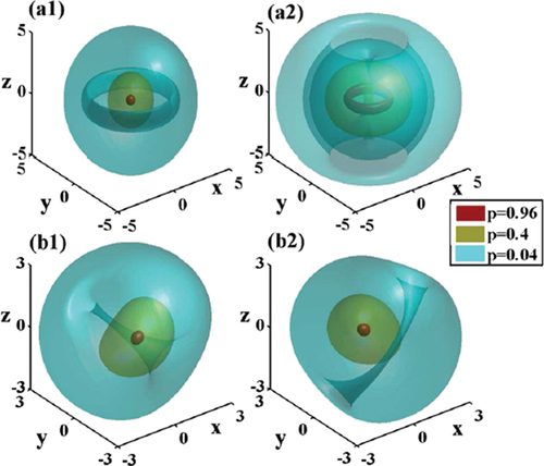
Figure 6. Density profiles of metastable 3D solitons with norm $N=8,$ produced by the numerical solution of Equation (47)(47) $[i\frac{\partial }{\partial t}+\frac{1}{2}{\mathrm{\nabla }}^2+i\lambda \mathrm{\nabla }\cdot \sigma +\left(\begin{array}{ll}|{\psi }_{+}{|}^2+\eta |{\psi }_{-}{|}^2& 0\\ 0& |{\psi }_{-}{|}^2+\eta |{\psi }_{+}{|}^2\end{array}\right)]\mathrm{\Psi }=0,$(47) . (a) An SV soliton for $\eta =0.3$, whose zero-vorticity and vortical components, $|{\psi }_{+}|$ and $|{\psi }_{-}|$, are plotted in (a1) and (a2), respectively. (b) An MM soliton for $\eta =1.5$, with (b1), (b2) displaying $|{\psi }_{+}|$ and $|{\psi }_{-}|$, respectively. In each subplot, different colors represent constant-magnitude surfaces, $|{\psi }_{\pm }|=(0.96,0.4,0.04)\times |{\psi }_{\pm }{|}_{\text{max}}$. The figure is borrowed from ref [77].

The mobility of the 3D solitons was addressed too, with the conclusion that, similar to the 2D case, steady motion is possible up to a certain maximum velocity, at which the amplitude of the soliton vanishes.

3. Emulation of the spin-orbit coupling (SOC) in optical systems

The similarity between GP equations for matter waves and NLS equations in optics suggests that many phenomena from the realm of BEC may be emulated in optics, including SOC [82,83]. In particular, it is possible to elaborate a counterpart for the matter-waves SOC in 2D systems in terms of light propagation in dual-core planar optical waveguides (couplers), with amplitudes of the electromagnetic waves in the two cores emulating two components of the BEC pseudo-spinor wave function. Assuming that each core carries intrinsic cubic self-focusing, it is possible to design optical setups which maintain stable 2D optical solitons in the spatiotemporal domain [84,85], in spite of the occurrence of the critical collapse in the same systems.

A crucially important feature of the SOC scheme in the binary BEC, which makes it possible to achieve the stabilization of the solitons, is that the linear mixing between the two components of the wave function in Equations (30)(30) $i\frac{\partial {\varphi }_{+}}{\partial t}=-\frac{1}{2}{\mathrm{\nabla }}^2{\varphi }_{+}-(|{\varphi }_{+}{|}^2+\gamma |{\varphi }_{-}{|}^2){\varphi }_{+}+(\lambda {\hat{D}}^{[-]}{\varphi }_{-}-i{\lambda }_D{\hat{D}}^{[+]}{\varphi }_{-})-\mathrm{\Omega }{\varphi }_{+},$(30) and (31(31) $i\frac{\partial {\varphi }_{-}}{\partial t}=-\frac{1}{2}{\mathrm{\nabla }}^2{\varphi }_{-}-(|{\varphi }_{-}{|}^2+\gamma |{\varphi }_{+}{|}^2){\varphi }_{-}-(\lambda {\hat{D}}^{[+]}{\varphi }_{+}+i{\lambda }_D{\hat{D}}^{[-]}{\varphi }_{+})+\mathrm{\Omega }{\varphi }_{-},$(31) ) is mediated by the terms with the first-order spatial derivatives. An optical system, which demonstrates the same feature, was elaborated in Ref [84] in terms of the spatiotemporal propagation of light in a planar dual-core coupler. As mentioned above, the amplitudes of the electromagnetic waves in the parallel cores, q₁ and q₂, emulate the two components of the pseudo-spinor wave function in the SOC BEC. In this case, the counterparts of the first spatial derivatives in Equations (30)(30) $i\frac{\partial {\varphi }_{+}}{\partial t}=-\frac{1}{2}{\mathrm{\nabla }}^2{\varphi }_{+}-(|{\varphi }_{+}{|}^2+\gamma |{\varphi }_{-}{|}^2){\varphi }_{+}+(\lambda {\hat{D}}^{[-]}{\varphi }_{-}-i{\lambda }_D{\hat{D}}^{[+]}{\varphi }_{-})-\mathrm{\Omega }{\varphi }_{+},$(30) and (31(31) $i\frac{\partial {\varphi }_{-}}{\partial t}=-\frac{1}{2}{\mathrm{\nabla }}^2{\varphi }_{-}-(|{\varphi }_{-}{|}^2+\gamma |{\varphi }_{+}{|}^2){\varphi }_{-}-(\lambda {\hat{D}}^{[+]}{\varphi }_{+}+i{\lambda }_D{\hat{D}}^{[-]}{\varphi }_{+})+\mathrm{\Omega }{\varphi }_{-},$(31) ) are time derivatives, which represent the temporal dispersion of the inter-core coupling. The respective system of NLS equation, written in the scaled form, is

(48) $i\frac{\partial q_1}{\partial \xi }+\frac{1}{2}(\frac{{\partial }^2{q}_1}{\partial {\eta }^2}+\frac{{\partial }^2{q}_1}{\partial {\tau }^2})-{\left|q_1\right|}^2{q}_1-(c+i\delta \frac{\partial }{\partial \tau })q_2-\beta q_1,$(48)

(49) $i\frac{\partial q_2}{\partial \xi }+\frac{1}{2}(\frac{{\partial }^2{q}_2}{\partial {\eta }^2}+\frac{{\partial }^2{q}_2}{\partial {\tau }^2})-{\left|q_2\right|}^2{q}_2-(c+i\delta \frac{\partial }{\partial \tau })q_1+\beta q_2,$(49)

where ξ and η are the propagation distance and transverse coordinate in the planar waveguide, τ is the temporal variable, while terms $\sim {\partial }^2/\partial {\eta }^2$ and ${\partial }^2/\partial {\tau }^2$ represent, respectively, the paraxial diffraction and anomalous GVD. Further, real c is the inter-core coupling, real δ accounts for the temporal dispersion of the coupling [86], and β, which is the counterpart of the ZS coefficient Ω in Equations (30)(30) $i\frac{\partial {\varphi }_{+}}{\partial t}=-\frac{1}{2}{\mathrm{\nabla }}^2{\varphi }_{+}-(|{\varphi }_{+}{|}^2+\gamma |{\varphi }_{-}{|}^2){\varphi }_{+}+(\lambda {\hat{D}}^{[-]}{\varphi }_{-}-i{\lambda }_D{\hat{D}}^{[+]}{\varphi }_{-})-\mathrm{\Omega }{\varphi }_{+},$(30) , represents possible asymmetry (refractive-index mismatch) between the optical cores. The model includes the usual intra-core Kerr nonlinearity, whose coefficient scaled to be 1. The SOC is emulated by the combination of the terms $\sim \delta$ and β.

Plane-wave solutions of the linearized version of Equations (48)(48) $i\frac{\partial q_1}{\partial \xi }+\frac{1}{2}(\frac{{\partial }^2{q}_1}{\partial {\eta }^2}+\frac{{\partial }^2{q}_1}{\partial {\tau }^2})-{\left|q_1\right|}^2{q}_1-(c+i\delta \frac{\partial }{\partial \tau })q_2-\beta q_1,$(48) and (49(49) $i\frac{\partial q_2}{\partial \xi }+\frac{1}{2}(\frac{{\partial }^2{q}_2}{\partial {\eta }^2}+\frac{{\partial }^2{q}_2}{\partial {\tau }^2})-{\left|q_2\right|}^2{q}_2-(c+i\delta \frac{\partial }{\partial \tau })q_1+\beta q_2,$(49) ) are looked for as $q_{1,2}\sim \exp (ik\xi -i\omega \tau +bz)$, where b is the propagation constant, k is the transverse wavenumber, and ω the excitation frequency. The resulting dispersion relation is

(50) $b_{\pm }=-\frac{1}{2}(k^2+{\omega }^2)\pm \sqrt{{\beta }^2+(c+\delta \cdot \omega {)}^2},$(50)

cf. Equation (32)(32) ${\mu }_{\pm }=\frac{k^2}{2}\pm \sqrt{({\lambda }^2+{\lambda }_D^2)k^2+4\lambda {\lambda }_D{k}_x{k}_y+{\mathrm{\Omega }}^2}.$(32) . Stationary soliton solutions of Equations (48(48) $i\frac{\partial q_1}{\partial \xi }+\frac{1}{2}(\frac{{\partial }^2{q}_1}{\partial {\eta }^2}+\frac{{\partial }^2{q}_1}{\partial {\tau }^2})-{\left|q_1\right|}^2{q}_1-(c+i\delta \frac{\partial }{\partial \tau })q_2-\beta q_1,$(48) ) and (49(49) $i\frac{\partial q_2}{\partial \xi }+\frac{1}{2}(\frac{{\partial }^2{q}_2}{\partial {\eta }^2}+\frac{{\partial }^2{q}_2}{\partial {\tau }^2})-{\left|q_2\right|}^2{q}_2-(c+i\delta \frac{\partial }{\partial \tau })q_1+\beta q_2,$(49) ) are looked for as

(51) $q_{1,2}=w_{1,2}(\tau ,\eta )\exp \left(ibz\right),$(51)

where $w_{1,2}$ are complex functions whose real parts are even with respect to η and τ, while the imaginary ones are even in η but odd in τ. A typical example of a stable soliton is displayed in Figure 7, with a bell-shaped $\left|w_1(\tau ,\eta )\right|$ and double-peaked $\left|w_2(\tau ,\eta )\right|$. The difference between the shapes of the components is similar to that between the zero-vorticity and vortex components of the SV soliton (41(41) ${\varphi }_{+}(x,y,t)=e^{-i\mu t}{f}_1(r^2),{\varphi }_{-}(x,y,t)=e^{-i\mu t+i\theta }r{f}_2(r^2),$(41) ).

Figure 7. An example of a stable spatiotemporal soliton produced by Equations (48)(48) $i\frac{\partial q_1}{\partial \xi }+\frac{1}{2}(\frac{{\partial }^2{q}_1}{\partial {\eta }^2}+\frac{{\partial }^2{q}_1}{\partial {\tau }^2})-{\left|q_1\right|}^2{q}_1-(c+i\delta \frac{\partial }{\partial \tau })q_2-\beta q_1,$(48) , (49(49) $i\frac{\partial q_2}{\partial \xi }+\frac{1}{2}(\frac{{\partial }^2{q}_2}{\partial {\eta }^2}+\frac{{\partial }^2{q}_2}{\partial {\tau }^2})-{\left|q_2\right|}^2{q}_2-(c+i\delta \frac{\partial }{\partial \tau })q_1+\beta q_2,$(49) ), and (51(51) $q_{1,2}=w_{1,2}(\tau ,\eta )\exp \left(ibz\right),$(51) ). The panels display absolute values of stationary fields w_1.2 and their real and imaginary parts. Parameters are $c=\delta =1$, $\beta =3$, and b = 1. The figure is borrowed from Ref [84].

Boundaries of the existence and stability domains for the solitons in parameter planes $(\delta ,b)$ and $(\beta ,\delta )$ are displayed in Figure 8. The existence (cutoff) boundaries, $b=b_{\mathrm{co}}$ and $\delta ={\delta }_{\mathrm{co}}$, which are marked in the plots, correspond to the edge of the linear spectrum (50(50) $b_{\pm }=-\frac{1}{2}(k^2+{\omega }^2)\pm \sqrt{{\beta }^2+(c+\delta \cdot \omega {)}^2},$(50) ), beyond which the solitons cannot exist. It is seen that the inter-core coupling dispersion, δ, and inter-core mismatch, β, are necessary for the stability of the 2D solitons. This conclusion is natural, because, as mentioned above, SOC in the dual-core optical system is emulated by the interplay of these factors, and 2D solitons cannot be stable in the absence of the SOC.

Figure 8. Existence and stability domains for the solitons generated by Equations (48)(48) $i\frac{\partial q_1}{\partial \xi }+\frac{1}{2}(\frac{{\partial }^2{q}_1}{\partial {\eta }^2}+\frac{{\partial }^2{q}_1}{\partial {\tau }^2})-{\left|q_1\right|}^2{q}_1-(c+i\delta \frac{\partial }{\partial \tau })q_2-\beta q_1,$(48) and (49(49) $i\frac{\partial q_2}{\partial \xi }+\frac{1}{2}(\frac{{\partial }^2{q}_2}{\partial {\eta }^2}+\frac{{\partial }^2{q}_2}{\partial {\tau }^2})-{\left|q_2\right|}^2{q}_2-(c+i\delta \frac{\partial }{\partial \tau })q_1+\beta q_2,$(49) ) in the plane of $(\delta ,b)$ (a), and $(\beta ,\delta )$(b). In (a), the solitons exist at $b>b_{\text{co}}$, and are stable at $b>b_{\text{cr}}$. In (b), they exist at $\delta >{\delta }_{\text{co}}$, being stable in the domain bounded by the red dots, labeled as ${\delta }_{\text{cr}}$. In both plots, c = 1. The figure is borrowed from Ref [84].

4. Quantum droplets

Among the settings that have recently been elaborated for the creation of multidimensional soliton-like modes, most advanced, as concerns the theory and experiment alike, is the work with QDs in atomic BEC. Theoretical predictions for fundamental and topologically structured stable QDs have been reported in many papers, starting from the pioneering work of Petrov [44], who considered a binary condensate with the inter-component attraction (imposed by means of the Feshbach resonance) slightly exceeding the intra-component self-repulsion. In the symmetric setting, with equal wave functions of the two components, the resulting 3D GP equation demonstrates weak cubic self-attraction. The stabilization against the supercritical collapse is provided by the correction to the MF approximation produced by quantum fluctuations around MF states. The correction was derived in 1957 by Lee, Huang, and Yang (LHY) [43]. As demonstrated by Petrov [44], in terms of the effective GP equation the LHY correction is represented by the quartic self-repulsive term, which arrests the development of the collapse. The balance between the inter-species MF cubic attraction and LHY-induced quartic repulsion gives rise to stable 3D and quasi-2D (’pancake-shaped’) localized bound states in the form of QDs (see review [56]). The prediction has been quickly confirmed by experimental observations of stable quasi-2D [46] and 3D [47] QDs in condensates of ³⁹K atoms, with the binary structure represented by a mixture of two different atomic states. QDs have also been created in single-component condensates of magnetic atoms, with long-range attraction provided by interactions between atomic magnetic moments in ultracold gases of erbium [87] and dysprosium [88].

The competition between the MF attraction and LHY repulsion admits atomic densities which cannot exceed a certain maximum value, thus making the condensate effectively incompressible. This is a reason why this quantum state of matter is identified as a superfluid, and localized states filled by it are called ’droplets’.

4.1. The theoretical models for QDs in three and two dimensions

The energy density of a binary BEC in the MF approximation is

(52) ${\mathcal{E}}_{\mathrm{MF}}=\frac{1}{2}{g}_{11}{n}_1^2+\frac{1}{2}{g}_{22}{n}_2^2+g_{12}{n}_1{n}_2,$(52)

where $g_{11,22}>0$ and $g_{12}<0$ are, respectively, strengths of the intra-component repulsion and inter-component attraction, and $n_{1,2}\equiv {\left|{\varphi }_{1,2}\right|}^2$ are densities of the two components, expressed in terms of the respective wave functions ${\varphi }_{1,2}$.

The LHY correction to the MF energy density (52(52) ${\mathcal{E}}_{\mathrm{MF}}=\frac{1}{2}{g}_{11}{n}_1^2+\frac{1}{2}{g}_{22}{n}_2^2+g_{12}{n}_1{n}_2,$(52) ), originating from the zero-point energy of Bogoliubov excitations around the MF state, takes the following form [44]:

(53) ${\mathcal{E}}_{\mathrm{LHY}}=\frac{64}{15\sqrt{\pi }}g{n}^2\sqrt{n{a}_s^3},$(53)

where $a_s>0$ is the s-wave scattering length, n is the density of both components, assuming that they are equal, $g\equiv 4\pi {\hslash }^{2}m/a_s$, and m is the atomic mass.

In a dilute condensate, the LHY term (53(53) ${\mathcal{E}}_{\mathrm{LHY}}=\frac{64}{15\sqrt{\pi }}g{n}^2\sqrt{n{a}_s^3},$(53) ) with scaling $\sim n^{5/2}$ is, generally, much smaller than the MF ones $\sim n^2$ in Equation (52)(52) ${\mathcal{E}}_{\mathrm{MF}}=\frac{1}{2}{g}_{11}{n}_1^2+\frac{1}{2}{g}_{22}{n}_2^2+g_{12}{n}_1{n}_2,$(52) . However, when the binary condensate is close to the equilibrium point, at which the MF self-repulsion is nearly balanced by the inter-component attraction, i.e. $0<-\delta g\equiv -(g_{12}+\sqrt{g_{11}{g}_{22}})\ll g_{11,22}$, the LHY correction is essential. The resulting system of LHY-amended GP equations for the wave functions of the 3D system can be written in a scaled form as

(54) $i\frac{\partial {\psi }_1}{\partial t}=-\frac{1}{2}{\mathrm{\nabla }}^2{\psi }_1+({\left|{\psi }_1\right|}^2+g_{\mathrm{LHY}}{\left|{\psi }_1\right|}^3){\psi }_1-g{\left|{\psi }_2\right|}^2{\psi }_1,$(54)

(55) $i\frac{\partial {\psi }_2}{\partial t}=-\frac{1}{2}{\mathrm{\nabla }}^2{\psi }_2+({\left|{\psi }_2\right|}^2+g_{\mathrm{LHY}}{\left|{\psi }_2\right|}^3){\psi }_2-g{\left|{\psi }_1\right|}^2{\psi }_2,$(55)

where the quartic self-repulsion terms with coefficient $g_{\mathrm{LHY}}$represent to the LHY correction to the MF, and g > 0 is the relative strength of the MF inter-component attraction.

The application of tight confinement to the condensate in one direction reduces the dimension from 3 to 2. The effective 2D LHY-corrected GP equation for the symmetric system, with ${\varphi }_1={\varphi }_2\equiv \varphi$, was derived in Ref [45]. In the scaled form, the 2D equation is

(56) $i\frac{\partial \varphi }{\partial t}=-\frac{1}{2}{\mathrm{\nabla }}^2\psi +\ln \left(|\varphi {|}^2\right)|\varphi {|}^2\varphi .$(56)

The increase of the local density from $|\varphi {|}^2<1$ to $|\varphi {|}^2>1$leads to the change of the sign of the logarithmic factor in Equation (56)(56) $i\frac{\partial \varphi }{\partial t}=-\frac{1}{2}{\mathrm{\nabla }}^2\psi +\ln \left(|\varphi {|}^2\right)|\varphi {|}^2\varphi .$(56) . As a result, the cubic term is self-attractive at small densities, initiating the spontaneous formation of QDs, and repulsive at large densities, arresting the transition to the collapse, thus stabilizing the 2D QDs.

4.2. 3D vortex QDs: theoretical results

Solutions of Equations (54)(54) $i\frac{\partial {\psi }_1}{\partial t}=-\frac{1}{2}{\mathrm{\nabla }}^2{\psi }_1+({\left|{\psi }_1\right|}^2+g_{\mathrm{LHY}}{\left|{\psi }_1\right|}^3){\psi }_1-g{\left|{\psi }_2\right|}^2{\psi }_1,$(54) and (55(55) $i\frac{\partial {\psi }_2}{\partial t}=-\frac{1}{2}{\mathrm{\nabla }}^2{\psi }_2+({\left|{\psi }_2\right|}^2+g_{\mathrm{LHY}}{\left|{\psi }_2\right|}^3){\psi }_2-g{\left|{\psi }_1\right|}^2{\psi }_2,$(55) ) for 3D vortex solitons, with equal components carrying chemical potential µ and integer winding number m, are looked for, in cylindrical coordinates $(\rho ,\theta ,z)$, as

(57) ${\psi }_1={\psi }_2=u(\rho ,z)\exp (-i\mu t+im\theta ),$(57)

where real function $u(\rho ,z)$ satisfies the equation

(58) $\mu u+\frac{1}{2}(\frac{{\partial }^2}{\partial {\rho }^2}+\frac{1}{\rho }\frac{\partial }{\partial \rho }+\frac{{\partial }^2}{\partial z^2}-\frac{m^2}{{\rho }^2})u+(g-1)u^3-g_{\mathrm{LHY}}{u}^4=0.$(58)

For given m, soliton families are characterized, as usual, by dependences of µ on the total norm, $N=4\pi {\int }_0^{\mathrm{\infty }}\rho d\rho {\int }_{-\mathrm{\infty }}^{+\mathrm{\infty }}dz{u}^2(\rho ,z)$. The families were constructed by means of a numerical solution [50]. The crucially important problem of their stability was addressed by means of a numerical solution of the linearized Bogoliubov – de Gennes equations for small perturbations around the stationary solitons, and the results were verified by means of direct simulations of Equations (54)(54) $i\frac{\partial {\psi }_1}{\partial t}=-\frac{1}{2}{\mathrm{\nabla }}^2{\psi }_1+({\left|{\psi }_1\right|}^2+g_{\mathrm{LHY}}{\left|{\psi }_1\right|}^3){\psi }_1-g{\left|{\psi }_2\right|}^2{\psi }_1,$(54) and (55(55) $i\frac{\partial {\psi }_2}{\partial t}=-\frac{1}{2}{\mathrm{\nabla }}^2{\psi }_2+({\left|{\psi }_2\right|}^2+g_{\mathrm{LHY}}{\left|{\psi }_2\right|}^3){\psi }_2-g{\left|{\psi }_1\right|}^2{\psi }_2,$(55) ) for the perturbed evolution.

The vortex QDs may be stable if their norm is large enough, which is a generic property of solitons supported by competing nonlinearities [89–91]. In turn, the QDs with a large norm are very broad, with a flat-top (FT) shape, see examples in Figure 9. In this limit, one may asymptotically neglect the terms $\sim {\rho }^{-1}$ and ρ⁻² in Equation (58)(58) $\mu u+\frac{1}{2}(\frac{{\partial }^2}{\partial {\rho }^2}+\frac{1}{\rho }\frac{\partial }{\partial \rho }+\frac{{\partial }^2}{\partial z^2}-\frac{m^2}{{\rho }^2})u+(g-1)u^3-g_{\mathrm{LHY}}{u}^4=0.$(58) , as well as ${\partial }^{2}u/\partial z^2$, reducing Equation (58)(58) $\mu u+\frac{1}{2}(\frac{{\partial }^2}{\partial {\rho }^2}+\frac{1}{\rho }\frac{\partial }{\partial \rho }+\frac{{\partial }^2}{\partial z^2}-\frac{m^2}{{\rho }^2})u+(g-1)u^3-g_{\mathrm{LHY}}{u}^4=0.$(58) to the quasi-1D form,

Figure 9. Isosurface density plots, at levels $|{\psi }_{1,2}{|}^2$ = 0.1 and $|{\psi }_{1,2}{|}^2$ = 0.5 in the top and bottom row, respectively, which demonstrate unstable and stable evolution of 3D symmetric (${\psi }_1={\psi }_2$) vortex QDs with winding numbers $m_{1,2}=1$, produced by simulations of Equations (54)(54) $i\frac{\partial {\psi }_1}{\partial t}=-\frac{1}{2}{\mathrm{\nabla }}^2{\psi }_1+({\left|{\psi }_1\right|}^2+g_{\mathrm{LHY}}{\left|{\psi }_1\right|}^3){\psi }_1-g{\left|{\psi }_2\right|}^2{\psi }_1,$(54) and (55(55) $i\frac{\partial {\psi }_2}{\partial t}=-\frac{1}{2}{\mathrm{\nabla }}^2{\psi }_2+({\left|{\psi }_2\right|}^2+g_{\mathrm{LHY}}{\left|{\psi }_2\right|}^3){\psi }_2-g{\left|{\psi }_1\right|}^2{\psi }_2,$(55) ) with $g_{\text{LHY}}=0.50$ and g = 1.75. Chemical potentials of the unstable and stable solutions are, respectively, ${\mu }_{1,2}=-0.04$ and ${\mu }_{1,2}=-0.16$. The figure is borrowed from Ref [50].

(59) $\mu u+\frac{1}{2}\frac{{\partial }^{2}u}{\partial {\rho }^2}+(g-1)u^3-g_{\mathrm{LHY}}{u}^4=0.$(59)

This equation seems as a formal equation of motion for a particle with coordinate u with respect to time ρ, which conserves the Hamiltonian,

(60) $\mathcal{H}=\frac{1}{4}{\left(\frac{\partial u}{\partial \rho }\right)}^2+\frac{\mu }{2}{u}^2+\frac{1}{4}(g-1)u^4-\frac{1}{5}{g}_{\mathrm{LHY}}{u}^5.$(60)

QD solutions, vanishing at $\rho \to \mathrm{\infty }$, correspond to $\mathcal{H}=0$. Finally, the FT solitons asymptotically correspond to setting ${\partial }^{2}u/\partial {\rho }^2=\partial u/\partial \rho =0$ in Equations (59)(59) $\mu u+\frac{1}{2}\frac{{\partial }^{2}u}{\partial {\rho }^2}+(g-1)u^3-g_{\mathrm{LHY}}{u}^4=0.$(59) and (60(60) $\mathcal{H}=\frac{1}{4}{\left(\frac{\partial u}{\partial \rho }\right)}^2+\frac{\mu }{2}{u}^2+\frac{1}{4}(g-1)u^4-\frac{1}{5}{g}_{\mathrm{LHY}}{u}^5.$(60) ) (with $\mathcal{H}=0$), which yields algebraic equations for the chemical potential and density u² of the asymptotically FT state inside the broad solitons. The resulting solution is

(61) ${\mu }_{\mathrm{FT}}=-\frac{25}{216}(g-1){\left(g_{\mathrm{LHY}}\right)}^{-2},{\left(u_{\mathrm{FT}}\right)}^2=\frac{25}{36}(g-1{)}^2{\left(g_{\mathrm{LHY}}\right)}^{-2}.$(61)

The QDs exist in interval $0<-\mu <-{\mu }_{\mathrm{FT}}$, with $N(\mu ={\mu }_{\mathrm{FT}})=\mathrm{\infty }$ (the divergence of the norm at $\mu \to {\mu }_{\mathrm{FT}}$ is a common feature of NLS equations with competing nonlinearities [92]). Further, ${\left(u_{\mathrm{FT}}\right)}^2$ is the largest density which these solutions may attain. As said above, the latter fact implies that the QDs are filled by the effectively incompressible quantum fluid. In the experimental realization of QDs, the density is $\sim {10}^{-8}$ g/cm³ [46,47], which is five orders of magnitude lower than the normal air density. In fact, the superfluid filling QDs is the most rarefied fluid known in nature [44].

The results produced for 3D QDs [50] are summarized in Figure 10, where panel (a) represents QD families with $m=0,1$ and 2 by means of the respective $N(\mu )$ curves, and (b) displays existence and stability boundaries ($N=N_{min}$ and $N=N_{\mathrm{st}}$, respectively) for the family with m = 1 in the $(g,N)$ plane. The fact that the 3D QDs exist above a minimum (threshold) value of N is generic for 3D models with competing self-attractive and repulsive nonlinearities [89]. In the area $N_{min}<N<N_{\mathrm{st}}$ in Figure 9 (b) the vortical QDs are unstable against spontaneous splitting, as shown in the top part of Figure 9. The stability-boundary value $N_{\mathrm{st}}$ rapidly increases with the decrease of g, and diverges at $g=g_{min}\approx 1.3$, all QDs with vorticity m = 1 being unstable at $g<g_{min}$.

Figure 10. (a) The norm versus the chemical potential for QDs with indicated values of the vorticity of both components, $m_1=m_2$, and parameters $g_{\text{LHY}}=0.5$ and g = 1.75 in Equations (54)(54) $i\frac{\partial {\psi }_1}{\partial t}=-\frac{1}{2}{\mathrm{\nabla }}^2{\psi }_1+({\left|{\psi }_1\right|}^2+g_{\mathrm{LHY}}{\left|{\psi }_1\right|}^3){\psi }_1-g{\left|{\psi }_2\right|}^2{\psi }_1,$(54) and (55(55) $i\frac{\partial {\psi }_2}{\partial t}=-\frac{1}{2}{\mathrm{\nabla }}^2{\psi }_2+({\left|{\psi }_2\right|}^2+g_{\mathrm{LHY}}{\left|{\psi }_2\right|}^3){\psi }_2-g{\left|{\psi }_1\right|}^2{\psi }_2,$(55) ). Red and black branches designate unstable and stable QDs, respectively, with red dots separating stable and unstable segments. For $m_{1,2}=2$, a stability segment exists too, but it is located at large values of N, outside of the region displayed in this panel. The dashed vertical line designates the value ${\mu }_{\text{FT}}$, given by Equation (61)(61) ${\mu }_{\mathrm{FT}}=-\frac{25}{216}(g-1){\left(g_{\mathrm{LHY}}\right)}^{-2},{\left(u_{\mathrm{FT}}\right)}^2=\frac{25}{36}(g-1{)}^2{\left(g_{\mathrm{LHY}}\right)}^{-2}.$(61) ), at which the QD’s norm diverges. (b) The bottom curve: the minimum norm, $N_{\text{min}}$, above which Equation (58)(58) $\mu u+\frac{1}{2}(\frac{{\partial }^2}{\partial {\rho }^2}+\frac{1}{\rho }\frac{\partial }{\partial \rho }+\frac{{\partial }^2}{\partial z^2}-\frac{m^2}{{\rho }^2})u+(g-1)u^3-g_{\mathrm{LHY}}{u}^4=0.$(58) produces the vortex-QD solutions with winding number m = 1, as a function of the attraction strength g. The top curve: the critical norm, $N_{\text{st}}$, above which the vortex QD is stable, vs. g. All the vortex states are unstable against spontaneous splitting at $g<g_{\text{min}}\approx 1.3$ ($N_{\text{st}}$ diverges at $g\to g_{\text{min}}$). In this panel, $g_{\text{LHY}}=0.5$ is fixed. The figure is borrowed from Ref [50].

Although the branch of the QD vortex states with m = 2 is completely unstable in the intervals of N and µ which are shown in Figure 10(a), these solutions become stable at still larger values of N and $-\mu$. For instance, the double-vortex QD is stable, with the same values g = 0.5 and $g_{\mathrm{LHY}}=1.75$ as fixed in 9(a), for $\mu =-0.183$ [50]. Plausibly, QDs with $m\ge 3$ and extremely large norms may be stable too, although they have not been found, as yet. This fact is explained by scaling

(62) $N_{\mathrm{st}}\sim m^6$(62)

for the lowest norm necessary for the stability of the vortex QDs in the 3D setting [49]. Indeed, this steep scaling makes it difficult to create stable QDs with $m\ge 3$.

It is also possible to consider the QD solutions of Equations (54)(54) $i\frac{\partial {\psi }_1}{\partial t}=-\frac{1}{2}{\mathrm{\nabla }}^2{\psi }_1+({\left|{\psi }_1\right|}^2+g_{\mathrm{LHY}}{\left|{\psi }_1\right|}^3){\psi }_1-g{\left|{\psi }_2\right|}^2{\psi }_1,$(54) and (55(55) $i\frac{\partial {\psi }_2}{\partial t}=-\frac{1}{2}{\mathrm{\nabla }}^2{\psi }_2+({\left|{\psi }_2\right|}^2+g_{\mathrm{LHY}}{\left|{\psi }_2\right|}^3){\psi }_2-g{\left|{\psi }_1\right|}^2{\psi }_2,$(55) ) with hidden vorticity (HV, i.e. opposite winding numbers in the two components and zero total angular momentum). They are defined, according to Ref [93], as

(63) ${\psi }_1=u(\rho ,z)\exp (-i\mu t+im\theta ),{\psi }_2=u(\rho ,z)\exp (-i\mu t-im\theta ),$(63)

where real function $u(\rho ,z)$ satisfies the same Equation (58)(58) $\mu u+\frac{1}{2}(\frac{{\partial }^2}{\partial {\rho }^2}+\frac{1}{\rho }\frac{\partial }{\partial \rho }+\frac{{\partial }^2}{\partial z^2}-\frac{m^2}{{\rho }^2})u+(g-1)u^3-g_{\mathrm{LHY}}{u}^4=0.$(58) as above. However, unlike the QDs with explicit vorticity, considered above, the HV ones are completely unstable against spontaneous splitting [50].

4.3. 2D vortex QDs

Solutions for 2D QDs, in the form of $\varphi =u\left(r\right)\exp (-i\mu t+iS\theta )$, and their stability were explored, on the basis of Equation (56)(56) $i\frac{\partial \varphi }{\partial t}=-\frac{1}{2}{\mathrm{\nabla }}^2\psi +\ln \left(|\varphi {|}^2\right)|\varphi {|}^2\varphi .$(56) , in Ref [49]. Here, $(r,\theta )$ are the polar coordinates, the integer vorticity is denoted as S, and real function u(r) satisfies the equation

(64) $\mu u+\frac{1}{2}(\frac{d^2}{d{r}^2}+\frac{1}{r}\frac{d}{dr}-\frac{S^2}{r^2})u+\ln \left(u^2\right)\cdot u^3=0,$(64)

cf. Equation (58)(58) $\mu u+\frac{1}{2}(\frac{{\partial }^2}{\partial {\rho }^2}+\frac{1}{\rho }\frac{\partial }{\partial \rho }+\frac{{\partial }^2}{\partial z^2}-\frac{m^2}{{\rho }^2})u+(g-1)u^3-g_{\mathrm{LHY}}{u}^4=0.$(58) . The limit (quasi-1D) form of Equation (64)(64) $\mu u+\frac{1}{2}(\frac{d^2}{d{r}^2}+\frac{1}{r}\frac{d}{dr}-\frac{S^2}{r^2})u+\ln \left(u^2\right)\cdot u^3=0,$(64) , corresponding to dropping terms $\sim r^{-1}$ and r⁻² (cf. Equation (59)(59) $\mu u+\frac{1}{2}\frac{{\partial }^{2}u}{\partial {\rho }^2}+(g-1)u^3-g_{\mathrm{LHY}}{u}^4=0.$(59) ), takes the form of a formal equation of motion with Hamiltonian

(65) ${\mathcal{H}}^{(2\mathrm{D})}=\frac{1}{4}{\left(\frac{du}{dr}\right)}^2+\frac{\mu }{2}{u}^2-\frac{1}{4}\ln \left(\frac{u^2}{\sqrt{e}}\right),$(65)

cf. Equation (60)(60) $\mathcal{H}=\frac{1}{4}{\left(\frac{\partial u}{\partial \rho }\right)}^2+\frac{\mu }{2}{u}^2+\frac{1}{4}(g-1)u^4-\frac{1}{5}{g}_{\mathrm{LHY}}{u}^5.$(60) . Similar to Equation (61)(61) ${\mu }_{\mathrm{FT}}=-\frac{25}{216}(g-1){\left(g_{\mathrm{LHY}}\right)}^{-2},{\left(u_{\mathrm{FT}}\right)}^2=\frac{25}{36}(g-1{)}^2{\left(g_{\mathrm{LHY}}\right)}^{-2}.$(61) in the 3D case, the quasi-1D reduction of Equation (64)(64) $\mu u+\frac{1}{2}(\frac{d^2}{d{r}^2}+\frac{1}{r}\frac{d}{dr}-\frac{S^2}{r^2})u+\ln \left(u^2\right)\cdot u^3=0,$(64) and (65(65) ${\mathcal{H}}^{(2\mathrm{D})}=\frac{1}{4}{\left(\frac{du}{dr}\right)}^2+\frac{\mu }{2}{u}^2-\frac{1}{4}\ln \left(\frac{u^2}{\sqrt{e}}\right),$(65) ) predicts the chemical potential and density of the 2D FT state (i.e. the largest attainable density for the 2D superfluid):

(66) ${\mu }_{\mathrm{FT}}^{(2\mathrm{D})}=-{\left(2\sqrt{e}\right)}^{-1}\approx -0.3033,{\left(u_{\mathrm{FT}}^{(2\mathrm{D})}\right)}^2=1/\sqrt{e}\approx 0.6065.$(66)

Numerical results demonstrate that 2D vortex QDs with a sufficiently large norm, $N=2\pi {\int }_0^{\mathrm{\infty }}{u}^2(r)rdr$, may be stable, at least, up to S = 5 [49]. Examples are displayed in Figure 11(a). The results are summarized in Figure 11(b) by plotting the lowest values of the norm which are necessary for the existence and stability of the 2D vortex QDs, viz., $N_{\text{min}}$ and $N_{\mathrm{th}}$, respectively. An analytical result is that $N_{\mathrm{th}}$ scales as

Figure 11. (a) Panels (a1)-(a4) display density patterns of 2D vortex QDs with $S=1,2,3,4$ and norm N = 1000, produced by the numerical solution of Equation (64)(64) $\mu u+\frac{1}{2}(\frac{d^2}{d{r}^2}+\frac{1}{r}\frac{d}{dr}-\frac{S^2}{r^2})u+\ln \left(u^2\right)\cdot u^3=0,$(64) . The states with $S=1,2,3$ are stable, while the one with S = 4 is unstable. (b) The minimum norm, $N_{\text{min}}$, necessary for the existence of the 2D vortex QDs (circles), and the threshold (critical) value of the norm, $N_{\text{th}}$, above which they are stable (triangles), vs. vorticity S. The results are produced by the numerical solution of Equation (56)(56) $i\frac{\partial \varphi }{\partial t}=-\frac{1}{2}{\mathrm{\nabla }}^2\psi +\ln \left(|\varphi {|}^2\right)|\varphi {|}^2\varphi .$(56) . The dashed curve shows the fit to the analytically predicted scaling (67(67) $N_{\mathrm{th}}^{(2\mathrm{D})}\sim S^4$(67) ), $N_{\text{th}}=6S^4$. The figure is borrowed from ref [89].

(67) $N_{\mathrm{th}}^{(2\mathrm{D})}\sim S^4$(67)

with the increase of S [49], cf. the steeper scaling in the 3D case, given by Equation (62)(62) $N_{\mathrm{st}}\sim m^6$(62) .

QDs of the HV type, corresponding to $m=\pm 1$ in the 2D version of Equation (63)(63) ${\psi }_1=u(\rho ,z)\exp (-i\mu t+im\theta ),{\psi }_2=u(\rho ,z)\exp (-i\mu t-im\theta ),$(63) , have their narrow stability region in the 2D model based on Equation (56)(56) $i\frac{\partial \varphi }{\partial t}=-\frac{1}{2}{\mathrm{\nabla }}^2\psi +\ln \left(|\varphi {|}^2\right)|\varphi {|}^2\varphi .$(56) , with norms $N>N_{\mathrm{th}}^{(\mathrm{HV})}\simeq 100$ [49], on the contrary to the full instability of the HV states in the 3D case, as mentioned above. However, all the 2D HV droplets with $|m|\ge 2$ are unstable.

A system of 2D GP equations, including both the LHY corrections and SOC (spin-orbit coupling) between the components, gives rise to vortex QDs of the MM type, which mix terms with S = 0 and +1 or -1 in the two components (see Equation (43)(43) ${\left({\varphi }_{+}^0\right)}_{\mathrm{MM}}=B_1{e}^{-{\beta }_1{r}^2}-B_{2}r{e}^{-i\theta -{\beta }_2{r}^2},{\left({\varphi }_{-}^0\right)}_{\mathrm{MM}}=B_1{e}^{-{\beta }_1{r}^2}+B_{2}r{e}^{i\theta -{\beta }_2{r}^2}.$(43) ). These QDs, which feature an anisotropic shape in 2D, are stable in a certain parameter region [94].

Vortex QDs in a condensate of magnetic atoms, with long-range dipole–dipole interactions, were theoretically investigated too and found to be completely unstable (unlike the results presented here) [95].

4.4. Experimental observations of QDs

The creation of stable QDs with a quasi-2D shape in a mixture of two different Zeeman states of ³⁹K atoms (’up’ and ‘down’ ones), namely,

(68) $|\uparrow ⟩\equiv |F,m_F⟩=|1,-1⟩\text{and }|\downarrow ⟩=|1,0⟩,$(68)

where F is the total angular momentum of the atom, and m_F is its z component, was first reported in Ref [46]. That work used a setup in which the QDs were self-trapped in the 2D planeand confined by a trapping potential in the transverse direction, making the QD shape oblate. The mixture is characterized by the respective scattering lengths, $a_{\uparrow \uparrow ,\downarrow \downarrow }>0$ and $a_{\uparrow \downarrow }<0$. The residual MF interaction was determined by

(69) $\delta a=a_{\uparrow \downarrow }+\sqrt{a_{\uparrow \uparrow }{a}_{\downarrow \downarrow }},$(69)

adjusted by means of the Feshbach resonance. As shown in Figure 12, the formation of stable oblate QDs, supported by the balance of MF attraction and LHY self-repulsion in the binary condensate, was observed in the case of $\delta a\approx -3.2a_0<0$, where $a_0\approx 0.0529$ nm is the Bohr radius. The same figure demonstrates a fast decay of the input in the absence of the attraction ($\delta a>0$), and the collapse of the single-component self-attractive condensate (a < 0).

Figure 12. The experimentally observed evolution of the condensates of³⁹K atoms in the oblate (quasi-2D) setting, displayed by means of density snapshots taken at different times t. Top: expansion of a the binary condensate in the absence of the effective MF attraction, with $\delta a=1.2a_0$ (see Equation (69)(69) $\delta a=a_{\uparrow \downarrow }+\sqrt{a_{\uparrow \uparrow }{a}_{\downarrow \downarrow }},$(69) ). Middle: the formation of a stable oblate QD in the binary condensate with the inter-component attraction, characterized by $\delta a=-3.2a_0<0$. Bottom: the collapse of a single-component self-attractive condensate, with scattering length $a=-2.06a_0$. The picture is borrowed from Ref [46].

Stable QDs in the 3D isotropic form were created in work [47], using the same atomic states (68(68) $|\uparrow ⟩\equiv |F,m_F⟩=|1,-1⟩\text{and }|\downarrow ⟩=|1,0⟩,$(68) ) as in Ref [46] and adjusting effective interactions by means of the Feshbach resonance. A holding potential, imposed by three mutually perpendicular red-detuned laser beams, was employed to prepare the condensate. In the case of $\delta a>0$ in Equation (69)(69) $\delta a=a_{\uparrow \downarrow }+\sqrt{a_{\uparrow \uparrow }{a}_{\downarrow \downarrow }},$(69) (MF repulsion), the initial state quickly expands after removing the holding potential, as shown in the top row of Figure 13. On the other hand, the bottom row demonstrates self-trapping of a stable isotropic QD under the action of the MF attraction, with $\delta a<0$.

Figure 13. Top: decay of the initial isotropic input in the absence of the MF attraction, with $\delta a>0$ in Equation (69)(69) $\delta a=a_{\uparrow \downarrow }+\sqrt{a_{\uparrow \uparrow }{a}_{\downarrow \downarrow }},$(69) . Bottom: the experimentally demonstrated formation of a stable isotropic QD in the case of the attraction, with $\delta a<0$ in Equation (69)(69) $\delta a=a_{\uparrow \downarrow }+\sqrt{a_{\uparrow \uparrow }{a}_{\downarrow \downarrow }},$(69) ). The horizontal axis represents time varying from t = 0 to 10 ms. The figure is borrowed from ref [47].

Both the oblate and isotropic QDs demonstrate rather short lifetimes, measured by few tens of milliseconds [46,47]. The lifetimes are limited by three-body collisions, which kick out atoms from the condensate into a thermal component of the gas.

The stable isotropic QDs can be readily set in motion by kicks, applied to them by laser pulses. This option suggests a possibility to study collisions between QDs moving in opposite directions, which was performed experimentally in Ref [96], using the same binary condensate of ³⁹K. Note that collisions of droplets of a classical fluid may lead to their merger into a single one, provided that the surface tension is sufficiently strong to absorb the kinetic energy of the colliding pair. Otherwise, the colliding droplets separate into two or more ones [97]. As shown in Figure 14, similar phenomenology is exhibited by the colliding QDs: merger of slowly moving droplets, and quasi-elastic mutual passage of faster ones. Similar results were demonstrated by simulations of the collisions in the framework of Equations (54)(54) $i\frac{\partial {\psi }_1}{\partial t}=-\frac{1}{2}{\mathrm{\nabla }}^2{\psi }_1+({\left|{\psi }_1\right|}^2+g_{\mathrm{LHY}}{\left|{\psi }_1\right|}^3){\psi }_1-g{\left|{\psi }_2\right|}^2{\psi }_1,$(54) and (55(55) $i\frac{\partial {\psi }_2}{\partial t}=-\frac{1}{2}{\mathrm{\nabla }}^2{\psi }_2+({\left|{\psi }_2\right|}^2+g_{\mathrm{LHY}}{\left|{\psi }_2\right|}^3){\psi }_2-g{\left|{\psi }_1\right|}^2{\psi }_2,$(55) ).

Figure 14. Experimentally observed collisions between moving isotropic QDs: (a) merger of slowly moving droplets; (b) passage of fast moving ones. The figure is borrowed from ref [96].

The mechanism stabilizing two-component QDs with MF inter-component attraction and LHY intra-component self-repulsion applies not only to binary systems composed of different hyperfine states of the same atom but also to heteronuclear mixtures. Experimentally, this possibility was realized in a mixture of⁴¹K and⁸⁷Rb atoms [48]. In particular, stable QDs were observed with the ratio of atom numbers $N_{\mathrm{K}}/N_{\mathrm{Rb}}\approx 0.8$, featuring lifetimes up to $\sim 100$ times longer than in the monatomic binary condensate.

5. Conclusion

This review is focused on selected topics for multidimensional solitons, which seem most relevant for the ongoing theoretical and experimental work in this vast area. These include stabilization of 2D and 3D SV and MM solitons by SOC in binary BECs, stabilization of 2D spatiotemporal optical solitons in dual-core planar waveguides by the photonic counterpart of SOC, and various theoretical and experimental results for 3D and 2D QDs (soliton-like states), stabilized by the LHY effect (quantum fluctuations around the MF states).

There are many other relevant aspects of studies of multidimensional solitons, which could not be included in this relatively short article. Most of them are presented in sufficient detail in the recently published book [7]. In addition to that, there are other significant topics related to this area, which are presented in other publications. In particular, this involves the propagation and self-trapping of spatiotemporal modes, including ones carrying the optical angular momentum, in multimode nonlinear optical fibers, for which the 3D NLS equation is a relevant model [98,99].

Also related to multidimensional solitons is nonlinear topological photonics, which addresses the propagation of topologically structured self-trapped modes in complex media [100,101]. In particular, a promising platform for the creation of 2D fundamental and topological optical solitons is provided by moiré superlattices, which are built as superpositions of simple lattices rotated with respect to each other [102–110]. In the general case, the 2D potentials created by the moiré structures are quasiperiodic. In this connection, it is relevant to mention that the interplay of 2D quasiperiodic lattices of the Penrose-tiling (pentagonal) type with the self-repulsive cubic nonlinearity can support stable fundamental and vortex species of gap solitons [111].

The recent progress in the work with multidimensional solitons has been fast, and there is vast space for further theoretical and experimental developments in this area.

Acronyms

1D	=	one-dimensional
2D	=	two-dimensional
3D	=	three-dimensional
BEC	=	Bose-Einstein condensate
CQ	=	cubic-quintic (nonlinearity))
FT	=	flat-top (profiles of solitons and quantum droplets)
GP	=	Gross-Pitaevskii (equation)
GS	=	ground state
GVD	=	group-velocity dispersion
LHY	=	Lee-Huang-Yang (correction to the MF theory)
MF	=	mean-field (approximation)
NLS	=	nonlinear Schr¨odinger (equation)
QD	=	quantum droplet
SOC	=	spin-orbit coupling
STOV	=	spatiotemporal vortex
TS	=	Townes soliton
VA	=	variational approximation
VK	=	Vakhitov-Kolokolov (stability criterion)
ZS	=	Zeeman splitting

Acknowledgments

I would like to thank my colleagues, with whom I collaborated on topics addressed in this review: F. Kh. Abdullaev, D. Anderson, G. Astrakharchik, C. B. de Araújo, B. B. Baizakov, W. B. Cardoso, G. Dong, N. Dror, P. D. Drummond, A. Gammal, Y. V. Kartashov, V. V. Konotop, H. Leblond, B. Li, Y. Li, M. Lisak, Z.-H. Luo, D. Mihalache, M. Modugno, W. Pang, M. A. Porras, H. Pu, J. Qin, A. S. Reyna, H. Sakaguchi, L. Salasnich, M. Salerno, E. Ya. Sherman, V. Skarka, D. V. Skryabin, L. Tarruell, L. Torner, F. Wise, L. G. Wright, and J. Zeng. I also thank Editors of Advances in Physics X, J. S. Aitchison, N. Balmforth, and R. Palmer, for their invitation to write this review article. My work on this topic was partly supported by the Israel Science Foundation through grant No. 1695/22.

Disclosure statement

No potential conflict of interest was reported by the author(s).

Additional information

Funding

This work was supported by the Israel Science Foundation [1695/22].

Notes

1. Sabbatical address.

References

- Makhankov VG, Rybakov YP, Sanyuk VI. The skyrme model: fundamentals, methods, applications. Berlin: Springer-Verlag; 1993.
- Houghton CJ, Manton NS, Sutcliffe PM. Rational maps, monopoles and skyrmions. Nucl Phys B. 1998;510:507–537. doi: 10.1016/S0550-3213(97)00619-6
- Manton N, Sutcliffe P. Topological solitons. Cambridge: Cambridge University Press; 2004.
- Radu E, Volkov MS. Stationary ring solitons in field theory — knots and vortons. Phys Rep. 2008;468:101–151. doi: 10.1016/j.physrep.2008.07.002
- Kartashov YV, Malomed BA, Shnir Y, et al. Twisted toroidal vortex-solitons in inhomogeneous media with repulsive nonlinearity. Phys Rev Lett. 2014;113:264101. doi: 10.1103/PhysRevLett.113.264101
- Biondini G, Pelinovsky D. Kadomtsev-Petviashvili equation, Scholarpedia. Scholarpedia. 2008;3:6539. doi: 10.4249/scholarpedia.6539
- Malomed BA. Multidimensional solitons. Melville, New York: AIP Publishing; 2022.
- Bergé L. Wave collapse in physics: principles and applications to light and plasma waves. Phys Rep. 1998;303:259–370. doi: 10.1016/S0370-1573(97)00092-6
- Sulem C, Sulem P-L. The nonlinear schrö dinger equation: self-focusing and wave collapse. New York: Springer; 1999.
- Zakharov VE, Kuznetsov EA. Solitons and collapses: two evolution scenarios of nonlinear wave systems. Phys Usp. 2012;55:535–556. doi: 10.3367/UFNe.0182.201206a.0569
- Fibich G. The nonlinear schrödinger equation: singular solutions and optical collapse. Heidelberg: Springer; 2015.
- Kivshar YS, Agrawal GP. Optical solitons: from fibers to photonic crystals. San Diego: Academic Press; 2003.
- Pitaevskii LP, Stringari S. Bose-Einstein condensation. Oxford: Oxford University Press; 2003.
- Silberberg Y. Collapse of optical pulses. Opt Lett. 1990;15:1282–1284. doi: 10.1364/OL.15.001282
- Abdullaev FK, Salerno M. Gap-Townes solitons and localized excitations in low-dimensional Bose-Einstein condensates in optical lattices. Phys Rev A. 2005;72:033617. doi: 10.1103/PhysRevA.72.033617
- Desaix M, Anderson D, Lisak M. Variational approach to collapse of optical pulses. J Opt Soc Am B. 1991;8:2082–2086. doi: 10.1364/JOSAB.8.002082
- Zakharov VE, Shabat AB. Exact theory of two-dimensional self-focusing and one-dimensional self-modulation of waves in nonlinear media, Zh. Eksp Teor Fiz. 1971;61:118–134. [English translation: J. Exp. Theor. Phys. 34, 62-69 (1972)].
- Kanashov AA, Rubenchik AM. On diffraction and dispersion effect on three-wave interaction. Physica D. 1981;4:122–134. doi: 10.1016/0167-2789(81)90009-9
- Hayata K, Koshiba M. Multidimensional solitons in quadratic nonlinear media. Phys Rev Lett. 1993;71:3275–3278. doi: 10.1103/PhysRevLett.71.3275
- Turitsyn SK. Stability of 2-dimensional and 3-dimensional optical solitons in a media with quadratic nonlinearity. JETP Lett. 1995;61:469–472.
- Malomed BA, Drummond P, He H, et al. Spatio-temporal solitons in optical media with a quadratic nonlinearity. Phys Rev E. 1997;56:4725–4735. doi: 10.1103/PhysRevE.56.4725
- Torruellas WE, Wang Z, Hagan DJ, et al. Observation of two-dimensional spatial solitary waves in a Quadratic Medium. Phys Rev Lett. 1995;74:5036–5039. doi: 10.1103/PhysRevLett.74.5036
- Liu X, Beckwitt K, Wise FW. Two-dimensional optical spatiotemporal solitons in quadratic media. Phys Rev E. 2000;62:1328–1340. doi: 10.1103/PhysRevE.62.1328
- Vlasov SN, Petrishchev VA, Talanov VI. Izv Vyssh Uchebn Zaved Radiofiz. 1971;14:1353. [English translation: Radiophys. Quantum Electron. 14, 1062 (1971)]. doi: 10.1007/BF01029467.
- Chiao RY, Garmire E, Townes CH. Self-trapping of optical beams. Phys Rev Lett. 1964;13:479–482. doi: 10.1103/PhysRevLett.13.479
- Vakhitov NG, Kolokolov AA. Stationary solutions of the wave equation in a medium with nonlinearity saturation, Radiophys. Radi Quan Elec. 1973;16:783–789. doi: 10.1007/BF01031343
- Chen C-A, Hung C-L. Observation of universal quench dynamics and Townes soliton formation from modulational instability in two-dimensional bose gases. Phys Rev Lett. 2020;125:250401. doi: 10.1103/PhysRevLett.125.250401
- Bakkali-Hassani B, Maury C, Zhou Y-Q, et al. Realization of a Townes soliton in a two-component planar bose gas. Phys Rev Lett. 2021;127:023603. doi: 10.1103/PhysRevLett.127.023603
- Chen C-A, Hung C-L. Observation of scale invariance in two-dimensional matter-wave Townes solitons. Phys Rev Lett. 2021;127:023604. doi: 10.1103/PhysRevLett.127.023604
- Zdagkas A, McDonnell C, Deng J, et al. Observation of toroidal pulses of light. Nat Photon. 2022;16:523–528. doi: 10.1038/s41566-022-01028-5
- Shen Y, Yu B, Wu H, et al. Topological transformation and free-space transport of photonic hopfions. Adv Phot. 2023;5:015001. doi: 10.1117/1.AP.5.1.015001
- Dror N, Malomed BA. Symmetric and asymmetric solitons and vortices in linearly coupled two-dimensional waveguides with the cubic-quintic nonlinearity. Physica D. 2011;240:526–541. doi: 10.1016/j.physd.2010.11.001
- Jhajj N, Larkin I, Rosenthal EW, et al. Spatiotemporal optical vortices. Phys Rev X. 2016;6:031037. doi: 10.1103/PhysRevX.6.031037
- Chong A, Wan C, Chen J, et al. Generation of spatiotemporal optical vortices with controllable transverse orbital angular momentum. Nat Photonics. 2020;14:350–354. doi: 10.1038/s41566-020-0587-z
- Bliokh KY. Spatiotemporal vortex pulses: Angular momenta and spin-orbit interaction. Phys Rev Lett. 2021;126:243601. doi: 10.1103/PhysRevLett.126.243601
- Porras MA. Transverse orbital angular momentum of spatiotemporal optical vortices, Progress in Electromagnetics Research. Prog Electromagn Res. 2023;177:95–105. doi: 10.2528/PIER23012203
- Malomed BA. INVITED) vortex solitons: old results and new perspectives. Physica D. 2019;399:108–137. doi: 10.1016/j.physd.2019.04.009
- Kruglov VI, Volkov VM, Vlasov RA, et al. Auto-waveguide propagation and the collapse of spiral light beams in non-linear media. J Phys A Math Gen. 1988;21:4381–4395. doi: 10.1088/0305-4470/21/23/020
- Qin J, Dong G, Malomed BA. Stable giant vortex annuli in microwave-coupled atomic condensates. Phys Rev A. 2016;94:053611. doi: 10.1103/PhysRevA.94.053611
- Firth WJ, Skryabin DV. Optical solitons carrying orbital angular momentum. Phys Rev Lett. 1997;79:2450–2453. doi: 10.1103/PhysRevLett.79.2450
- Falcão Filho L, de Araújo CB, Boudebs G, et al. Robust two-dimensional spatial solitons in liquid carbon disulfide. Phys Rev Lett. 2013;110:013901. doi: 10.1103/PhysRevLett.110.013901
- Reyna AS, Boudebs G, Malomed BA, et al. Robust self-trapping of vortex beams in a saturable optical medium. Phys Rev A. 2016;93:013840. doi: 10.1103/PhysRevA.93.013840
- Lee TD, Huang K, Yang CN. Eigenvalues and eigenfunctions of a Bose system of hard spheres and its low-temperature properties. Phys Rev. 1957;106:1135–1145. doi: 10.1103/PhysRev.106.1135
- Petrov DS. Quantum mechanical stabilization of a collapsing Bose-Bose mixture. Phys Rev Lett. 2015;115:155302. doi: 10.1103/PhysRevLett.115.155302
- Petrov DS, Astrakharchik GE. Ultradilute low-dimensional liquids. Phys Rev Lett. 2016;117:100401. doi: 10.1103/PhysRevLett.117.100401
- Cabrera C, Tanzi L, Sanz J, et al. Quantum liquid droplets in a mixture of Bose-Einstein condensates. Science. 2018;359:301–304. doi: 10.1126/science.aao5686
- Semeghini G, Ferioli G, Masi L, et al. Self-bound quantum droplets of atomic mixtures in free space? Phys Rev Lett. 2018;120:235301. doi: 10.1103/PhysRevLett.120.235301
- D’Errico C, Burchianti A, Prevedelli M, et al. Observation of quantum droplets in a heteronuclear bosonic mixture. Phys Rev Res. 2019;1:033155. doi: 10.1103/PhysRevResearch.1.033155
- Li Y, Chen Z, Luo Z, et al. Two-dimensional vortex quantum droplets. Phys Rev A. 2018;98:063602. doi: 10.1103/PhysRevA.98.063602
- Kartashov YV, Malomed BA, Tarruell L, et al. Three-dimensional droplets of swirling superfluids. Phys Rev A. 2018;98:013612. doi: 10.1103/PhysRevA.98.013612
- Malomed BA, Mihalache D, Wise F, et al. Spatiotemporal optical solitons. J Optics B: Quant Semicl Opt. 2005;7:R53–R72. doi: 10.1088/1464-4266/7/5/R02
- Kartashov YV, Malomed BA, Torner L. Solitons in nonlinear lattices. Rev Mod Phys. 2011;83:247–305. doi: 10.1103/RevModPhys.83.247
- Malomed BA, Mihalache L, Wise F, et al. Viewpoint: on multidimensional solitons and their legacy in contemporary atomic, molecular and optical physics. J Phys B At Mol Opt Phys. 2016;49:170502. doi: 10.1088/0953-4075/49/17/170502
- Malomed BA. Multidimensional solitons: well-established results and novel findings. Eur Phys J Spec Top. 2016;225:2507–2532. doi: 10.1140/epjst/e2016-60025-y
- Kartashov Y, Astrakharchik G, Malomed B, et al. Frontiers in multidimensional self-trapping of nonlinear fields and matter. Nat Rev Phys. 2019;1:185–197. doi: 10.1038/s42254-019-0025-7
- Luo Z-H, Pang W, Liu B, et al. A new form of liquid matter: quantum droplets. Front Phys. 2021;16:32501. doi: 10.1007/s11467-020-1020-2
- Malomed BA. Multidimensional dissipative solitons and solitary vortices. Chaos, Solitons & Fractals. 2022;163:112526. doi: 10.1016/j.chaos.2022.112526
- Hauke P, Cucchietti FM, Tagliacozzo L, et al. Can one trust quantum simulators? Rep Prog Phys. 2012;75:082401. doi: 10.1088/0034-4885/75/8/082401
- Lin Y-J, Jiménez-García K, Spielman IB. Spin–orbit-coupled Bose–Einstein condensates. Nature. 2011;471:83–86. doi: 10.1038/nature09887
- Galitski V, Spielman IB. Spin–orbit coupling in quantum gases. Nature. 2013;494:49–54. doi: 10.1038/nature11841
- Campbell DL, Juzeliūnas G, Spielman IB. Realistic Rashba and Dresselhaus spin-orbit coupling for neutral atoms. Phys Rev A. 2011;84:025602. doi: 10.1103/PhysRevA.84.025602
- Dresselhaus G. Spin-orbit coupling effects in zinc blende structures. Phys Rev. 1955;100:580–586. doi: 10.1103/PhysRev.100.580
- Bychkov YA, Rashba EI. Oscillatory effects and the magnetic susceptibility of carriers in inversion layers. J Phys C Solid State Phys. 1984;17:6039–6045. doi: 10.1088/0022-3719/17/33/015
- Wu Z, Zhang L, Sun W, et al. Realization of two-dimensional spin-orbit coupling for Bose-Einstein condensates. Science. 2016;354:83–88. doi: 10.1126/science.aaf6689
- Kawakami T, Mizushima T, Machida K. Textures oF F = 2 spinor Bose-Einstein condensates with spin-orbit coupling. Phys Rev A. 2011;84:011607(R. doi: 10.1103/PhysRevA.84.011607
- Ramachandhran B, Opanchuk B, Liu X-J, et al. Half-quantum vortex state in a spin-orbit-coupled Bose-Einstein condensate. Phys Rev A. 2012;85:023606. doi: 10.1103/PhysRevA.85.023606
- Sakaguchi H, Li B. Vortex lattice solutions to the Gross-Pitaevskii equation with spin-orbit coupling in optical lattices. Phys Rev A. 2013;87:015602. doi: 10.1103/PhysRevA.87.015602
- Conduit GJ. Line of Dirac monopoles embedded in a Bose-Einstein condensate. Phys Rev A. 2012;86:021605(R. doi: 10.1103/PhysRevA.86.021605
- Wu CJ, Mondragon-Shem I, Zhou X-F. Unconventional Bose—Einstein condensations from spin-orbit coupling. Chin Phys Lett. 2011;28:097102. doi: 10.1088/0256-307X/28/9/097102
- Kawakami T, Mizushima T, Nitta M, et al. Stable skyrmions in SU(2) gauged Bose-Einstein condensates. Phys Rev Lett. 2012;109:015301. doi: 10.1103/PhysRevLett.109.015301
- Sakaguchi H, Li B, Malomed BA. Creation of two-dimensional composite solitons in spin-orbit-coupled self-attractive Bose-Einstein condensates in free space. Phys Rev E. 2014;89:032920. doi: 10.1103/PhysRevE.89.032920
- Salasnich L, Cardoso WB, Malomed BA. Localized modes in quasi-two-dimensional Bose-Einstein condensates with spin-orbit and Rabi couplings. Phys Rev A. 2014;90:033629. doi: 10.1103/PhysRevA.90.033629
- Sakaguchi H, Malomed BA. Discrete and continuum composite solitons in Bose-Einstein condensates with the Rashba spin-orbit coupling in one and two dimensions. Phys Rev E. 2014;90:062922. doi: 10.1103/PhysRevE.90.062922
- Sakaguchi H, Sherman EY, Malomed BA. Vortex solitons in two-dimensional spin-orbit coupled Bose-Einstein condensates: effects of the Rashba-Dresselhaus coupling and the Zeeman splitting. Phys Rev E. 2016;94:032202. doi: 10.1103/PhysRevE.94.032202
- Sakaguchi H, Li B, Sherman EY, et al. Composite solitons in two-dimensional spin-orbit coupled self-attractive Bose-Einstein condensates in free space. Roman Rep Phys. 2018;70:502.
- Mardonov S, Sherman EY, Muga JG, et al. Collapse of spin-orbit-coupled Bose-Einstein condensates. Phys Rev A. 2015;91:043604. doi: 10.1103/PhysRevA.91.043604
- Zhang Y-C, Zhou Z-W, Malomed BA, et al. Stable solitons in three dimensional free space without the ground state: self-trapped Bose-Einstein condensates with spin-orbit coupling. Phys Rev Lett. 2015b;115:253902. doi: 10.1103/PhysRevLett.115.253902
- Sakaguchi H, Malomed BA. One- and two-dimensional gap solitons in spin-orbit-coupled systems with Zeeman splitting. Phys Rev A. 2018;97:013607. doi: 10.1103/PhysRevA.97.013607
- Landau LD, Lifshitz EM. Quantum mechanics: nonrelativistic theory. Moscow: Moscow (Nauka Publishers; 1974.
- Manakov SV. On the theory of two-dimensional stationary self-focusing of electromagnetic waves. Zh Eksp Teor Fiz. 1973;65:505–516.
- Zhou XF, Li Y, Cai Z, et al. Unconventional states of bosons with the synthetic spin–orbit coupling. J Phys B At Mol Opt Phys. 2013;46:134001. doi: 10.1088/0953-4075/46/13/134001
- Bliokh KY, Rodríguez-Fortu Ña FJ, Nori F, et al. Spin–orbit interactions of light. Nat Photonics. 2015;9:796–808. doi: 10.1038/nphoton.2015.201
- Liu G, Zhang X, Zhang X, et al. Spin-orbit rabi oscillations in optically synthesized magnetic fields. Light Sci Appl. 2023;12:205. doi: 10.1038/s41377-023-01238-8
- Kartashov YV, Malomed BA, Konotop VV, et al. Stabilization of solitons in bulk Kerr media by dispersive coupling. Opt Lett. 2015;40:1045–1048. doi: 10.1364/OL.40.001045
- Sakaguchi H, Malomed BA. One-and two-dimensional solitons in-symmetric systems emulating spin–orbit coupling. New J Phys. 2016;18:105005.
- Chiang KS. Intermodal dispersion in two-core optical fibers. Opt Lett. 1995;20:997–999. doi: 10.1364/OL.20.000997
- Chomaz L, Baier S, Petter D, et al. Quantum-fluctuation-driven crossover from a dilute Bose-Einstein condensate to a macrodroplet in a dipolar quantum fluid. Phys Rev X. 2016;6:041039. doi: 10.1103/PhysRevX.6.041039
- Schmitt M, Wenzel M, Böttcher F, et al. Self-bound droplets of a dilute magnetic quantum liquid, nature. Nature. 2016;539:259–262. doi: 10.1038/nature20126
- Mihalache D, Mazilu D, Crasovan L-C, et al. Stable spinning optical solitons in three dimensions. Phys Rev Lett. 2002;88:073902. doi: 10.1103/PhysRevLett.88.073902
- Quiroga-Teixeiro M, Michinel H. Stable azimuthal stationary state in quintic nonlinear optical media. J Opt Soc Am B. 1997;14:2004–2009. doi: 10.1364/JOSAB.14.002004
- Pego RL, Warchall HA. Spectrally stable encapsulated vortices for nonlinear Schrödinger equations. J Nonlinear Sci. 2002;12:347–394. doi: 10.1007/s00332-002-0475-3
- Pushkarov KI, Pushkarov DI, Tomov IV. Self-action of light beams in nonlinear media: soliton solutions. Opt Quant Electr. 1979;11:471–478. doi: 10.1007/BF00620372
- Brtka M, Gammal A, Malomed BA. Hidden vorticity in binary Bose-Einstein condensates. Phys Rev A. 2010;82:053610. doi: 10.1103/PhysRevA.82.053610
- Li Y, Luo Z, Liu Y, et al. Two-dimensional solitons and quantum droplets supported by competing self- and cross-interactions in spin-orbit-coupled condensates. New J Phys. 2017b;19:113043. doi: 10.1088/1367-2630/aa983b
- Cidrim A, dos Santos FEA, Henn EAL, et al. Vortices in self-bound dipolar droplets. Phys Rev A. 2018;98:023618. doi: 10.1103/PhysRevA.98.023618
- Ferioli G, Semeghini G, Masi L, et al. Collisions of self-bound quantum droplets. Phys Rev Lett. 2019;122:090401. doi: 10.1103/PhysRevLett.122.090401
- Pan KL, Law CK, Zhou B. Experimental and mechanistic description of merging and bouncing in head-on binary droplet collision. J Appl Phys. 2008;103:06490. doi: 10.1063/1.2841055
- Krupa K, Tonello A, Barthélémy A, et al. Multimode nonlinear fiber optics, a spatiotemporal avenue. APL Photonics. 2019;4:110901. doi: 10.1063/1.5119434
- Ma M, Lian Y, Wang Y, et al. Generation, transmission and application of orbital angular momentum in optical fiber: a review. Front Phys. 2021;9:773505. doi: 10.3389/fphy.2021.773505
- Bandres MA, Rechtsman MC, Segev M. Topological photonic quasicrystals: fractal topological spectrum and protected transport. Phys Rev X. 2016;6:011016. doi: 10.1103/PhysRevX.6.011016
- Smirnova D, Leykam D, Chong YD, et al. Nonlinear topological photonics. Appl Phys Rev. 2020;7:021306. doi: 10.1063/1.5142397
- Wang P, Zheng Y, Chen X, et al. Localization and delocalization of light in photonic moiré lattices. Nature (London). 2020;577:42–46. doi: 10.1038/s41586-019-1851-6
- Fu Q, Wang P, Huang C, et al. Optical soliton formation controlled by angle twisting in photonic moiré lattices. Nat Photonics. 2020;14:663–668. doi: 10.1038/s41566-020-0679-9
- Kartashov YV, Ye F, Konotop VV, et al. Multifrequency solitons in commensurate-incommensurate photonic moiré lattices. Phys Rev Lett. 2021;127:163902. doi: 10.1103/PhysRevLett.127.163902
- Kartashov YV. Light bullets in moiré lattices. Opt Lett. 2022;47:4528–4531. doi: 10.1364/OL.471022
- Ivanov SK, Konotop VV, Kartashov YV, et al. Vortex solitons in moiré optical lattices. Opt Lett. 2023;48:3797–3800. doi: 10.1364/OL.494681
- Arkhipova AA, Kartashov YV, Ivanov SK, et al. Observation of linear and nonlinear light localization at the edges of moiré arrays. Phys Rev Lett. 2023;130:083801. doi: 10.1103/PhysRevLett.130.083801
- Liu X, Zeng J. Gap solitons in parity–time symmetric moiré optical lattices. Photonics Res. 2023;11:196–202. doi: 10.1364/PRJ.474527
- Liu X, Zeng J. Matter-wave gap solitons and vortices of dense Bose-Einstein condensates in moiré optical lattices. Chaos, Solitons & Fractals. 2023;174:113869. doi: 10.1016/j.chaos.2023.113869
- Li Z-Y, Li J-H, Zhao Y, et al. Robust light bullets in Rydberg gases with moiré lattice. Results Phys. 2023;53:106990. doi: 10.1016/j.rinp.2023.106990
- Sakaguchi H, Malomed BA. Gap solitons in quasiperiodic optical lattices. Phys Rev E. 2006;74:026601. doi: 10.1103/PhysRevE.74.026601