Statistical Modeling of Spatially Stratified Heterogeneous Data

Abstract

Spatial statistics is an important methodology for geospatial data analysis. It has evolved to handle spatially autocorrelated data and spatially (locally) heterogeneous data, which aim to capture the first and second laws of geography, respectively. Examples of spatially stratified heterogeneity (SSH) include climatic zones and land-use types. Methods for such data are relatively underdeveloped compared to the first two properties. The presence of SSH is evidence that nature is lawful and structured rather than purely random. This induces another “layer” of causality underlying variations observed in geographical data. In this article, we go beyond traditional cluster-based approaches and propose a unified approach for SSH in which we provide an equation for SSH, display how SSH is a source of bias in spatial sampling and confounding in spatial modeling, detect nonlinear stochastic causality inherited in SSH distribution, quantify general interaction identified by overlaying two SSH distributions, perform spatial prediction based on SSH, develop a new measure for spatial goodness of fit, and enhance global modeling by integrating them with an SSH q statistic. The research advances statistical theory and methods for dealing with SSH data, thereby offering a new toolbox for spatial data analysis.

空间统计是地理空间数据分析的重要方法, 能够处理空间自相关数据和空间(局部)异质数据, 从而捕捉地学第一定律和第二定律。空间分层异质性(SSH)的例子包括气候带和土地利用类型。与前两个特性相比, 很少有针对此类数据的方法。SSH的存在, 证明了自然是有规则的、结构化的, 而非完全随机的。这引发了地理数据差异背后的“一层”因果关系。本文超越传统的聚类方法, 提出整体性SSH方法, 提供了SSH方程, 展示了SSH如何导致空间采样的偏差和空间建模的混淆, 检测了SSH分布中的非线性随机因果关系, 对两个SSH分布叠加所识别的交互作用进行了量化, 基于SSH进行了空间预测, 开发了新的空间拟合度指标, 并将其与SSH的q统计相结合从而改进了全局建模。该研究促进了SSH数据处理的统计学理论和方法, 为空间数据分析提供了新方法。

La estadística espacial es una valiosa metodología para el análisis de datos geoespaciales. Este campo ha evolucionado para ocuparse del manejo de datos espacialmente autocorrelacionados y datos espacialmente (localmente) heterogéneos, que buscan captar las primera y segunda leyes de la geografía, respectivamente. Ejemplos de la heterogeneidad estratificada espacialmente (SSH) incluyen las zonas climáticas y los tipos de usos del suelo. Los métodos para ese tipo de datos son relativamente subdesarrollados, comparados con las dos primeras propiedades. La presencia de la SSH es evidencia de que la naturaleza se rige por leyes y está estructurada en vez de ser puramente aleatoria. Esto induce otra “capa” de causalidad que subraya las variaciones observadas en los datos geográficos. En este artículo nos adentramos más allá de los enfoques tradicionales basados en conglomerados y proponemos un enfoque unificado para la SSH en el cual proveemos una ecuación para la SSH, indicamos cómo la SSH es una fuente de sesgo en el muestreo espacial y de confusión en la modelización espacial, detectamos la causalidad estocástica no lineal en la distribución de la SSH, cuantificamos la interacción general identificada por medio de la superposición de dos distribuciones de SSH, formulamos una predicción espacial basada en la SSH, desarrollamos una nueva medida para la bondad de ajuste espacial y mejoramos la modelización global integrando todo con una estadística q de SSH. La investigación contribuye al avance de la teoría estadística y de los métodos para tratar con datos de SSH, entregando de ese modo una nueva caja de herramientas para el análisis de datos espaciales.

Key Words:

• confounding
• inference
• sample bias
• spatial causality
• spatially stratified heterogeneity

关键词:

• 混淆
• 推理
• 样本偏差
• 空间因果关系
• 空间分层异质性

Palabras clave:

• causalidad espacial
• confusión
• heterogeneidad estratificada espacialmente
• inferencia
• sesgo muestral

Statistical theory was initially developed for independently and identically distributed (iid) observations from a population (often obtained by a series of experiments). Spatial data, resulting from variables of interest that are close to each other in a geographical space, tend to be similar locally, however. This is called the spatially autocorrelated (SAC) property in the literature. If the underlying spatial variations from the population can be described by a spatial statistical model, then statistical inference becomes possible (see, e.g., Christakos 1992; Griffith 2003; Haining 2003). Modeling spatial dependency, by some form of spatial autoregressive model for lattice data, or permissible semivariogram for geostatistical data, lies at the heart of many branches of spatial statistics (Cliff and Ord 1981; Cressie 1993; Stein 2022).

The ability to model spatial dependency opens opportunities to undertaking many forms of spatial analysis, such as spatial interpolation (Matheron 1963). The underlying principle can be described as one of borrowing nearby data values by inverse distance weighting for the purpose of estimating remaining data values to construct a map. Models of spatial variations can also be used to improve the precision of small area parameter estimates by similar processes of borrowing information from neighboring areas. The underlying assumption that allows this form of information borrowing is that neighboring parameter values are similar so that the information contained in the data from neighboring areas can be “borrowed” for estimating the unknown parameters (Ripley 1981; Fotheringham, Brunsdon, and Charlton 2000; Rao 2003; Goldstein 2011; Haining and Li 2020).

This article is concerned with the development of methods that can address another frequently encountered property of spatial data: spatial heterogeneity. Heterogeneity is a term used in statistics to indicate that one or more statistical characteristics of interest are not the same across all subsets of the population (Everitt and Skrondal 2010, 204). The presence of spatial heterogeneity violates the second part of the iid assumption—observations are not “identically distributed.” In particular, if our study region is large and physically or socioeconomically diverse or our study region is observed in high spatial resolution, then the assumption that all subsets of the study region have the same statistical characteristics is likely to be violated. The assumption that some of the subsets of our data have different statistical characteristics might be a safer starting point in data analysis. For instance, Dutilleul (2011, 20–21) described three types of often encountered spatial heterogeneity: heterogeneity in the mean (or first-order heterogeneity; see Stein, Hoogerwerf, and Bouma 1988; Fotheringham, Brunsdon, and Charlton 2000; Lloyd 2010; Ge et al. 2019; Haining and Li 2020, chapter 6), heterogeneity in the variance (heteroscedasticity or second-order heterogeneity), and heterogeneity associated with the autocorrelation structure of the data (see Getis and Ord 1992; Anselin 1995; Kulldorff 1997).

Another ubiquitous form of heterogeneity is spatially stratified heterogeneity (SSH; J. F. Wang, Zhang, and Fu 2016). It arises when an area comprising a collection of contiguous spatial units can be partitioned into distinct spatial segments (strata) where within each stratum (each comprising a number of spatial units) the mean of a variable or the association between the observations is the same, indicating that each stratum only displays within-stratum homogeneity. The statistical characteristics might not be the same when compared with other strata so that the strata display between-strata heterogeneity collectively. This problem seems to have received less systematic attention than other forms of spatial heterogeneity described earlier. Part of the reason for this might lie in the challenge of identifying homogeneous zones. Stein, Hoogerwerf, and Bouma (1988) appears to be the first paper to address spatial stratification—a topic to which we return in the following sections of this article. Modeling would be confounded if it did not make allowance for SSH when population is SSH (Simpson Paradox). Even if SSH is recognized, there might be insufficient data to provide nice estimates of the parameters in each stratum using traditional estimation methods—referred to as the data sparsity problem, or the biased sample problem when not all strata have been sampled (see, e.g., Meng 2018; J. Wang et al. 2018; Bradley et al. 2021). Besides the challenges raised by the presence of SSH, disregarding the presence of SSH implies that some of the information in the data, which could be useful in that data’s analysis, is not being exploited.

This article aims through theory and with reference to previous studies to promote a systematic framework for the statistical analysis and modeling of SSH. The article is structured as follows. We first consider the principal statistical challenges that arise when working with SSH populations. We then introduce the equation for SSH populations aiming to address the challenge of identifying SSH zones. Next, we give examples of statistical inference for SSH populations. We then draw the reader’s attention to a number of applications where SSH is a key issue for data analysis due to the nature of the scientific problem. We comment here on the relationship between SSH and the methods of this article on the one hand and the modifiable areal unit problem (MAUP) on the other. We draw some final conclusions and directions for future work to conclude.

Statistical Challenges When Working with Spatially Stratified Heterogeneous Populations

In this section we illustrate statistical problems that can arise if SSH goes undetected in the process of a statistical analysis.

Unrepresentative Samples and Poor Quality Estimates

An unrepresentative sample means that the histogram of the sample differs significantly from that of the population from which it is collected. In this case the expected value of the sample mean would be not identical to the population mean; that is, the sample mean would be a biased estimator of the population mean. If the population is SSH and the sample size is small with few or no sample points in some strata, then this will exacerbate the problem of estimator bias. If there are few sample points in a stratum, then large estimates of error variances would appear.

Figure 1 shows a well-known biased sampling problem: the distribution of climatic zones within China and the distribution of meteorological stations in China in 1900. The inadequacy of the early network of stations for statistical analysis of the whole country is obvious. Supplementary information, if available, could be called on to reduce the effects of any intrastratum sample bias (Heckman 1979; J. Wang et al. 2018). If a population is spatially homogeneous, then the mean square error (MSE) of the estimator declines as the sample size corresponding to a given level of spatial autocorrelation increases (Rodríguez-Iturbe and Mejía 1974; O’Connell et al. 1979).

Figure 1. Climate zones in China (spatially stratified heterogeneity [SSH] population) and meteorological stations (sample) in 1900.

Confounded Relationships

The presence of SSH undermines inferences based on global statistics that disregard any stratified heterogeneities in the population (Lindley and Novick 1981; Hox 2010, 3). For example, L. Xu et al. (2011) used bubonic plague records and climate records for the period from 1850 to 1964 to show that the intensity of plague in China presents no clear evidence of an association with wetness levels until the data are broken down into the northern and southern halves of the country. Figure 2A shows a plot based on a data set for the whole country, whereas Figures 2B and 2C partition the data into North China and South China. L. Xu et al. (2011) found that plague-carrying rodent communities respond differently to higher levels of precipitation in arid northern China compared with humid southern China.

Figure 2. The relationship between plague intensity and wetness levels. (A) All China; (B) only North China; (C) only South China. The solid curves are the generalized additive model associations. Their linear trends are represented by dotted red lines. Plague intensity refers to the number of plague cases (N) per year. Source: Figures 2B and 2C are reproduced with the permission of L. Xu et al. (2011).

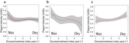
Analogously, if the population were SSH, then any global model based on a pooling of data sets would give rise to errors in prediction for either the entire area or a few subareas without the user necessarily knowing which subsets they are. In a special issue of the Canadian Water Resources Journal, overviewing processes that generate flooding in Canada, Buttle et al. (2016) reported that a global model cannot provide accurate flood predictions for both entire and different regions of Canada subjected to different climatic regimes. Different flood-generating processes include flooding generated by snowmelt, rain-on-snow, and rainfall, as well as groundwater flood processes and flooding induced by storm surges, ice jams, and urban flooding.

The two major challenges of bias and confounding in spatial statistics mentioned earlier cannot be automatically solved by big data and artificial intelligence, and in fact they could be made worse due to the “big data paradox” (Meng 2018; Li et al. 2023). In fact, they could be solved more straightforwardly if the SSH was identified prior to modeling. This would allow statistics to be calculated individually within strata to avoid confounding or by using the Heckman (Heckman 1979) or B-SHADE (J. F. Wang, Hu, et al. 2013; C. Xu et al. 2022) methods. If a large national survey is carried out but SSH is not considered, then the foregoing problems can be addressed by Bayesian hierarchical models (BHMs) if the relationships in strata are monotonic, which allows the “borrowing information” methodology referred to earlier (see Ripley 1981, 19–27; Dunn and Harrison 1993; Haining and Li 2020, chapters 7 and 8).

Equation for Spatially Stratified Heterogeneity

In this section, we illustrate SSH (Figure 3), which is then represented in an equation form. This facilitates the investigation of a statistic that is a function of (L, P), where L represents the number of strata and P represents the form of the partition into the strata.

Figure 3. Illustrative maps displaying different amounts of spatially stratified heterogeneity (see text) together with the corresponding values of the q-statistic. *p < 0.05. **p < 0.01.

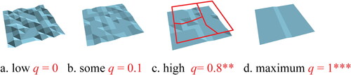
Figure 3 illustrates a range of maps displaying data values with different degrees of spatial structures. Figure 3A represents a map that shows no evidence of stratification. Figure 3B illustrates a map with some small degrees of spatial structures (some spatial autocorrelation between neighboring values) but still showing no evidence of any stratification. Figure 3D shows a map with two sharply defined strata showing strong homogeneity within each of the strata (little or no intrastrata variability). Figure 3C depicts an “imperfectly stratified heterogeneous” map where data values are well structured in space with some within-strata variations and the boundary lines (in red) between the three strata. These are somewhat fuzzy—appearing to be three spatial regimes, although the positions of the boundary lines could be debated. In practice, Figure 3C represents the most likely scenario. Attached to each map in Figure 3 is a notional value of what is termed the q-statistic, which provides an appropriate measure of SSH. We discuss this q-statistic next.

An Equation for an SSH Population

An SSH (super)population is composed of strata (h = 1, … , L). We do not assume that stratification is known, implying that it is not a regression problem. Therefore, we also need to estimate stratification in our method. For a given stratification, the SSH equation can be expressed as: (1) $$\mathbf{y}=\mathbf{X}\mathit{\beta }+\mathbf{e},\mathbf{e}\sim N(\mathbf{0},{\sigma }^2\mathbf{I})$$(1) where y = (y₁, · · ·, y_L)^T and y_h = (y_h1, · · ·, $y_{h{N}_h}$)^T. X = diag(1_N1, · · ·, 1_NL), 1_Nh is the Nh-dimensional column vector with all of its components equal to 1, β = (M₁, …, M_L)^T, and e = (e₁, · · ·, e_L)^T with e_h = (e_h1, · · ·, $e_{h{N}_h}$)^T. X partitions data into L strata in which stratum h is of size N_h and an element vector y_h and a mean µ_h. If a linear regression approach is used (Gujarati and Porter 2009, 37), then X cannot be changed and would be updated. In the SSH equation, however, adding or changing a stratum denoted by X would require changing the definitions of some of the strata X. We have: (2a) $$\mathit{\text{SST}}=\mathit{\text{SSB}}+\mathit{\text{SSW}}$$(2a) (2b) $$\mathit{\text{SST}}={\mathbf{y}}^{\mathrm{T}}\left(\mathbf{I}-\mathbf{B}\right)\mathbf{y}$$(2b) (2c) $$\mathit{\text{SSB}}={\mathbf{y}}^{\mathrm{T}}\left(\mathbf{A}-\mathbf{B}\right)\mathbf{y}$$(2c) (2d) $$\mathit{\text{SSW}}={\mathbf{y}}^{\mathrm{T}}\left(\mathbf{I}-\mathbf{A}\right)\mathbf{y}$$(2d) where A = X(X^TX)⁻¹X ^T, B = 1(1^T1)⁻¹1^T, and 1 is the N-dimensional vector with all components equal to 1. Given X, SST, SSB, and SSW represent the sum of squares total, the sum of squares between strata, and the sum of squares within strata, respectively. Note that A – B is an orthogonal projection matrix and tr(I – A) = N – L. Equations 2b(2b) $$\mathit{\text{SST}}={\mathbf{y}}^{\mathrm{T}}\left(\mathbf{I}-\mathbf{B}\right)\mathbf{y}$$(2b) , 2c(2c) $$\mathit{\text{SSB}}={\mathbf{y}}^{\mathrm{T}}\left(\mathbf{A}-\mathbf{B}\right)\mathbf{y}$$(2c) , and 2d(2d) $$\mathit{\text{SSW}}={\mathbf{y}}^{\mathrm{T}}\left(\mathbf{I}-\mathbf{A}\right)\mathbf{y}$$(2d) can only be derived based on a given stratification. To identify the true stratification, we need to combine them together. This motivates us to propose a function for SSH.

A Function for SSH

A measure of SSH (J. F. Wang, Zhang, and Fu 2016) can be generalized and investigated as a function of L and P based on the matrix form: (3) $$q\left(L,P\right)=1‐\mathrm{ }\frac{{\mathbf{y}}^T\left(\mathbf{I}-\mathbf{A}\right)\mathbf{y}}{{\mathbf{y}}^T\left(\mathbf{I}-\mathbf{B}\right)\mathbf{y}}$$(3)

We here make explicit that the q-statistic is a function of the number of strata (L) and the form of the particular partition (P) as there are many partitions that can produce L strata. An optimized stratification can be defined by (4) $$\mathrm{O}\left(L,P\right)={\text{argmax}}_{(L,P)}\left\{q(L,P)\right\}$$(4)

One more essential difference between the R² for linear regression or the interclass correlation coefficient (ICC) and our q-function given by Equation 3(3) $$q\left(L,P\right)=1‐\mathrm{ }\frac{{\mathbf{y}}^T\left(\mathbf{I}-\mathbf{A}\right)\mathbf{y}}{{\mathbf{y}}^T\left(\mathbf{I}-\mathbf{B}\right)\mathbf{y}}$$(3) is that R² or ICC assumes that the partition is given, but here we do not make this assumption. It follows that the q-statistic has a noncentral F distribution given X (J. F. Wang, Zhang, and Fu 2016), whereas ICC follows the standard central F distribution (Snijders and Bosker 2011, 46). The q function is used to detect SSH and to make attribution for SSH without requiring any linearity assumption. This is also different from R² and ICC for multilevel modeling. In Figure 4, we illustrate the q-function. For emphasis we have shown that stratum h = 1 appears in two distinct geographical areas. The stratum label refers to its clustering (e.g., land-use type), not its spatial location. The stratification of a variable Y can be partitioned either by Y itself or by a suspected explanatory variable X (discussed later), depending on the purpose of the study. This result holds for other forms of stratification such as in time if data values are temporal.

Figure 4. Illustrating the q-function. N and σ² are the number of units and variance of an area, respectively; subscript h = 1, … , L, is the h-stratum; SSH of a population Y is partitioned by either itself Y or its explanatory variable X.

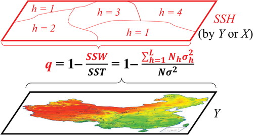
The q-function, for any given L and P, takes a value in the interval [0, 1], where 0 reflects no stratified heterogeneity. This implies that each of the L strata has the same degree of (internal) heterogeneity as found across the whole map (Figure 3A). A value of the q-function equal to 1 indicates complete within-stratum homogeneity (all data values within a stratum are the same), which implies that the heterogeneity observed across the whole map is due to the differences between the L strata for the given partition (Figure 3D).

Evaluation of Different Stratifications

The identification of zones lies at the heart of traditional regional geography as well as contemporary data analysis practice concerned with boundary delineation (e.g., wombling; see Womble 1951) and various forms of regional clustering or “region-building” (Longley et al. 2005, 135; Dutilleul 2011, 20–21). As the stratification is unknown, we want to find a stratification strategy to provide the minimum within-group variation value simultaneously with the maximum between-group variation value. The boundary between the strata might exist already, such as geological maps and climate zones, although they could be reassessed and revised by new tools; or could be determined through searches using optimal algorithms, or is divided by equal intervals, as provide by ArcGIS settings. The choice among the approaches is based on the context of the study. In the case of spatial classifiers (Haining 2003, 201–06), the objective function in these methods is usually constructed by combining a homogeneity function for within-group variances and a spatial compactness function for their coordinate locations. The q-function can be treated as the first of these functions. The advantage of the q-statistic, as we shall see, is that it is possible to connect the null distribution with a standard, well-known, distribution such that we can easily derive its p value.

The q-statistic can be used to make an empirical evaluation of different stratifications (varying L or varying the partition for the same value of L) to see which yields the largest value of the statistic. Taking the case where L is fixed (we are confident about the number of strata) and we want to compare two partitions P1 and P2 that yield L strata, we compute: (5) $$\mathit{Q}\left(P\mathit{1},P\mathit{2}\right)=q\left(L;P\mathit{1}\right)–q\left(L;P\mathit{2}\right).$$(5)

If $Q$(P1, P2) > 0 (< 0) then P1 (P2) yields a more homogeneous intrastratum partition than P2 (P1). Because $Q$(P1, P2) = $\frac{\mathit{\text{SSB}}1-\mathit{\text{SSB}}2}{\mathit{\text{SST}}}$ = $\frac{D\left(P1,P2\right)}{\mathit{\text{SST}}},$ the statistical significance of the difference between the two partitions can be tested by D(P1, P2). If P1 is the true stratification, then it can be shown that: (6) $$D\left(P\mathit{1},P\mathit{2}\right){\sim }^{\text{approximate}}N\left(E\left(D\right),V\left(D\right)\right)$$(6) with (7) $$E\left(D\right)={\sigma }^2\text{tr}\left(\mathbf{A}1–\mathbf{A}2\right)+{\mathit{\beta }}^{\mathrm{T}}{\mathbf{X}}_1{}^{\mathrm{T}}\left(\mathbf{A}1–\mathbf{A}2\right){\mathbf{X}}_1\mathit{\beta }$$(7) (8) $$V\left(D\right)=\text{2tr}{\left(\mathbf{A}1–\mathbf{A}2\right)}^2+\text{4}{\mathit{\beta }}^{\mathrm{T}}{\mathbf{X}}_1{}^{\mathrm{T}}{\left(\mathbf{A}1–\mathbf{A}2\right)}^2{\mathbf{X}}_1\mathit{\beta }$$(8) where E and V stand for expectation and variance, respectively; A1 and A2 are A for P1 and P2, respectively; and X₁ is X for one of the partitions, P1, say. Although there might be many partitions generating L strata, in practice the number of partitions that will justify comparison should be much fewer in number.

The individual elements of q(L; P), SSW_h, that is the sum of squares within stratum h and is the L terms in the numerator of the second term in the definition of q(L; P) in Equation 3(3) $$q\left(L,P\right)=1‐\mathrm{ }\frac{{\mathbf{y}}^T\left(\mathbf{I}-\mathbf{A}\right)\mathbf{y}}{{\mathbf{y}}^T\left(\mathbf{I}-\mathbf{B}\right)\mathbf{y}}$$(3) , can be compared to see which of these strata displays the most (intrastratum) heterogeneity. The strata making the largest contribution to the numerator might be candidates for further partitioning—that is the increase of L. Comparing partitions involving different numbers of strata raises another problem, however; namely the need to include a penalty to prevent overstratification. The argument is similar to that encountered when selecting independent variables in a regression model where Akaike’s information criterion (AIC) is used to compare different models allowing for differences in model complexity. A model, A, with more independent variables than another, B, where the independent variables in B form a subset of those in A, will fit the data better but be more complex and this needs to be allowed for when model fits are compared—in this case two stratifications with a different number of strata are identified. AIC penalized estimation based on minimized Kullback–Leibler information between two probability density functions (PDFs; Akaike 1974) might be not used directly to compare two stratifications that differ in terms of L. Figure 5 illustrates that spatial statistics become necessary to distinguish various spatial arrangements that possess the same marginal PDF or histogram. Consequently, different SSHs (either partitions or the number of strata, or both) could share the same AIC. Furthermore, giving the SSH of the population (patterns composed of the blue and white pixels in Figure 5), the effects of each boundary choice (red lines in Figures 5B and 5C), MAUP, are measured by the q-statistic.

Figure 5. Schematic comparison between classical statistics and spatial statistics. Three spatial distributions measured using classical statistics (mean value $\overline{y}$ and variance σ²), spatially autocorrelated Moran’s I (Moran 1950) and spatially stratified heterogeneity q-statistic (with strata partitioned by red lines). Three 8 × 8 pixel boxes displaying the same number of blue (value 1) and white (value 0) pixels (N_w = N_B = 32). q₁ and q₂ refer to the q values for the population stratified by line 1 and line 2, respectively, q_1&2 refers to the q value for the population stratified by lines 1 and 2. Source: Adopted with revisions from J. F. Wang, Zhang, and Fu (2016).

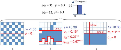
SSH is the characteristic of a population (gray background in Figures 3 and 5, and the bottom layer of Figure 4), which is first identified by a researcher or team of researchers imposing a stratification on the data (stratified by red lines in Figures 3–5) and then measured by the q(L, P) statistic. The best stratification is the one that accurately reflects the SSH of the population. In practice, hundreds of algorithms have been developed to help find the best stratification. Table 1 illustrates how the SSH information propagates from SSH population (q₀ ∈ [0, 1], 0 if the population is iid and 1 for perfect SSH) to a stratification by a researcher (Ψ ∈ [0, 1], 0 if population SSH is completely disregarded and 1 for fully accounted for), which is then measured by q. In essence, q = Ψq₀. The case that q = 1 indicates the population displays perfect SSH (q₀ = 1), which is also fully identified by the stratification (Ψ = 1; Figure 5C stratified by line 1); the case that q = 0 indicates either the population being iid (Figures 3A and 5A) or that SSH population has been poorly stratified (Figure 5C stratified by line 2). The case that q value lies between 0 and 1 reflects an SSH between the two extremes above (Figure 5B stratified by line 1 or line 2 or both).

Table 1. Spatially stratified heterogeneity (SSH) population and its representation by stratification

q = Ψq0		SSH of population
		Perfect SSH q0 = 1	q0 = (0, 1)	iid q0 = 0
Stratification Ψ	True Ψ = 1	1		0
	Ψ = (0, 1)
	Neglected Ψ = 0	0		0

Note: iid = independently and identically distributed.

A population might be SSH from one perspective but not from another. For example, Figure 5A displays perfect SSH with two strata of gray and white, but no SSH from the perspective of a geospatial zonation partitioned by the red line (q = 0). Sometimes, the interpretability of the findings is more important than maximizing q(L, P). For example, in analyzing economic data variation, established standards of stratification (L, P), such as the UN’s standard for levels of gross domestic product per capita, might be chosen to conform with a preexisting methodology.

Inference under Spatially Stratified Heterogeneity

In this section, we provide examples of statistical analysis when SSH is present in a data set.

Statistics within Homogeneous Strata

Once a partition into homogeneous strata has been constructed under the case when observations are independent, conventional statistics can then be applied to draw inferences about intrastrata properties as the previous example illustrates (see Figures 2B and 2C). If, on the other hand, intrastratum observations are SAC, then spatial statistical techniques are needed to draw inferences about intrastrata properties. Because many of these statistics depend on the specification of a weights (or connectivity) matrix W (Haining and Li 2020, chapter 4) for spatial relationships between the observations, a question arises as to how to treat those observations close to the boundary of any stratum. In the interest of improving statistical precision (particularly if a stratum has relatively few observations), it might be appropriate to “borrow” some sample observations from the “other side” of the stratum boundary. Although this might introduce some bias into parameter estimators, such an approach might be justified, especially in those situations where some segments of a stratum boundary are more akin to zones of transition, even if other boundary segments display abrupt change. An attempt to resolve such a question is to estimate the nonzero entries in the W matrix (Haining and Li 2020, 4.10 and 8.4). Kriging with a moving window and geographically weighted regression (GWR) would be alternative choices for spatial interpolation to points when the population is SSH. The two approaches potentially risk large error at SSH boundaries, because both approaches are based on drawing on neighboring samples. Yang et al. (2022) merged two water basins (two strata) to form a single homogeneous area when their SSH was tested to be insignificant to reduce errors in soil interpolation (Stein, Hoogerwerf, and Bouma 1988).

When interest centers on the spatial distribution of some parameter, Haining and Li (2020, chapters 7 and 8) described a number of BHMs with spatial dependency that yield estimates of a heterogeneous parameter. They illustrate an application of these methods to samples of household income for Newcastle-upon-Tyne, England at the middle super-output area (MSOA) level. An MSOA is a small area for reporting UK Census data, which is treated as a single stratum by our method. A sample is collected from a national survey such that not all MSOAs (strata) have data or many of them only have a small number of observations. The samples within each stratum are assumed to be conditionally independent and identically distributed, that is, conditional on the underlying process generating the data. It is the set of MSOA-level parameter values that are SAC. The application involves different autoregressive models for capturing spatial autocorrelation in the spatial distribution of the parameter of interest (average household income at the MSOA level). The chosen model, specified in the BHM’s prior model for the parameter of interest, leads to information sharing across the MSOAs. BHMs are fitted using Markov chain Monte Carlo simulation. Here as in the cases of the other methods described earlier, additional covariates can be included in the model to improve the accuracy of the estimates.

Spatial Interpolation with SSH

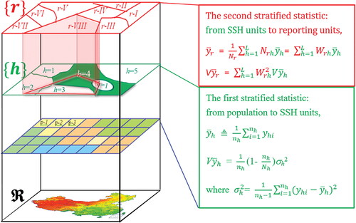
Areal interpolation is the term used to describe the process of transferring data from one spatial framework (“the source”) to a new spatial framework (“the target” or “reporting” framework); see, for example, Goodchild, Anselin, and Deichmann (1993), Haining (2003, 131–38), and Lin, Xu, and Wang (2023) for an overview. J. F. Wang, Haining, et al. (2013) described what they termed “the sandwich method” to transfer data values from a source to a target framework appropriate for an SSH population (Figure 6). The methodology provides estimates for each target zone with an estimate of error variance. First, the SSH population is stratified into homogeneous strata (J. F. Wang, Haining, and Cao 2010) and mean and variance estimates are obtained for each of the source strata ({h} in Figure 6). Next, the SSH population of source zones is overlaid on the target zone framework ({r} in Figure 6). The estimates for the target zones are obtained from the source zones in proportion to the degree of overlap occurring. Any individual source zone can contribute to the estimates of multiple target zones. In this sense, the sandwich approach “borrows strength” from all the source strata that overlap any particular target stratum, depending on the geographical extent and configuration of the source zones relative to the target zones. This process of borrowing strength might not be limited to just nearby areas. Provided that there are sample values in each source zone, the methodology can be applied without the need of whether they belong to sample data in a target unit. According to the definition of q and stratified sampling, the overall error of the sandwich estimator can be easily derived: mse($\overline{y}$) = (1 – q)(1 – $\frac{n}{N}$) $\frac{{\sigma }^2}{n},$ where n and N stand for the number of units in the sample and population, respectively, and σ² is the variance. Clearly, the error is zero if q = 1 and collapses into the error of the sample mean if q = 0.

Figure 6. Illustrating the sandwich estimator when the population is spatially stratified heterogenous (SSH). A population ℜ is composed of strata {h = 1, ., L} and reporting units {r}. The green shaded area in {h} takes the example of stratum h = 4. The red transparent prism between {h} and {r} illustrates information flowing from {h} to {r}; $\overline{y}$ and V$\overline{y}$ stand for mean and variance of the attribute y, respectively; n and N stand for the number of sample units and all units in a stratum, respectively. Subscript h stands for stratum h, hi stands for the ith sample unit in stratum h; subscript rh stands for a unit formed by the intersection between two units r and h.

A number of techniques are proposed to construct maps of spatial distributions of some SSH attributes (e.g., annual air temperature by climatic zones) on the basis of a sample of SAC observations. Means of surface with nonhomogeneity (MSN), biased sentinel hospital area disease estimator (B-SHADE), and single-point area (SPA) estimators combine Kriging and stratified sampling to make inferences that are best linear unbiased (BLUE). MSN is applicable when all strata have samples (J. F. Wang, Christakos, and Hu 2009; Hu and Wang 2011; Gao et al. 2015). The estimator reduces to either Kriging if SSH is absent or the sandwich estimator (J. F. Wang, Haining, et al. 2013) if SAC is absent. When some strata have no observations, B-SHADE can be used to make a spatial prediction by the ratio between a sample and the population. This ratio could be estimated using a covariate. For example, the ratio in the early years when stations are sparse in number can be estimated by the observations from present-day meteorological stations to adjust for sample bias (J. F. Wang et al. 2011; Hu et al. 2013; C. D. Xu, Wang, and Li 2018). B-SHADE reduces to MSN if all strata have samples. When only a single sample unit is available, SPA estimates an areal mean using a prior relationship that has been identified between the target variable (e.g., PM2.5) and a covariate (e.g., PM10) that has been observed in all strata (J. F. Wang, Hu, et al. 2013).

Spatial Causality

Establishing cause-and-effect associations between variables is a core interest for scientific researchers (Einstein 1953), including both deterministic and stochastic causations (Christakos 2012). By spatial stochastic causality inferred from spatial characteristics, Christakos (2012) coined the term stochastic causality to refer to the case where if anything happens at location A, then something related will happen at location B with a certain probability, where B might or might not be spatially coincident with A. Causality inferences based on binary intervention or no intervention in natural experiments (Imbens and Rubin 2015; Pearl and Mackenzie 2018) and using SAC data (Gao et al. 2023) were developed, respectively.

Spatial patterns might provide insights into causality. Snow (1854) mapped the association between the residential locations of individual deaths from cholera and the sites of the Broad Street pumps from which people living in this area obtained their water. He observed that the number of deaths from cholera decreased with increasing distance from the pump (Figure 7C). A more recent story of spatial causality is the identification of a seafood market as a possible source of COVID-19 in Wuhan City, China. This was done by noting that the mass center of the cases, rather than that of the citizens in a city, is significantly closer to the market. The second support is that the hot spot map of cases is exactly consistent with the location of the market. The third support is that the circle centered at the market, with the radius equal to the median distance between the cases and the market, is much smaller than the circle centered at the market with the radius equal to the median distance between the human population to the market (Worobey et al. 2022).

Figure 7. Association between (A) two points’ pairs (Pearson 1895), (B) two time series (Zhang et al. 2007), and (C–D) two spatial patterns (Snow 1854; Wang et al. 2010): From correlation (A) to causality (B–D). The Pearson coefficient is around 0.7 for both (A) and (B), but (B) has an extra piece of information of the consistency between two nonmonotonous trends. (C) displays the spatial consistence between the cases density (y) and the distance to a well (x) in a cholera outbreak in London in 1854. (D) displays the consistency between two complicated spatial patterns formed by the prevalence of neural birth defects (y) and lithology zones (x), respectively. The coupling is measured by spatially stratified heterogeneity q-statistic.

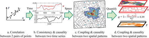
Our axiom is that if X causes Y, then their spatial patterns (spatial stratified heterogeneities) would tend to be coupled, in addition to displaying a significant Pearson’s correlation. A version of the function q(L; P) can be used to examine the coupling, as hinted at in Figure 4. In Figure 4 we note that the partition, P, can be specified in terms of the observed values of Y, which is the variable to be tested for stratified heterogeneity, or it could be specified in terms of a suspected explanatory variable, say X. To make clear which variable is used to construct the partition, we could write q(L; Px) when the partition is based on some variable X. This variable, X, might be either categorical, such as a land-use type, or quantitative with the property that the values of X within any of the X-defined strata are similar but far away between strata. Suppose that we are able to specify a partition, Px, of a quantitative variable X. The mean value of X within a single stratum defines the level of X in that stratum and all the observed values of X in that same stratum are similar. If there is causality between Y and X across the strata then the value of the function, call it q(L; Px), calculated on Y will tend to be large (closer to 1). On the other hand, if there is no causality between Y and X, the value of q(L; Px), calculated on Y will tend to be small (closer to 0). This is because if X causes Y then, within the strata, we should expect Y to be homogeneous in the strata of X. In other words, their spatial patterns, depicted by stratifications (L; Px), tend to be coupled. The degree of the consistency can be measured by q(L; Px) of y.

The correspondence between two geographical shapes might be indicative of a causal association (Sugihara et al. 2012). Figure 7 illustrates different graphical forms that could be suggestive of spatial causality. Figure 7A shows a linear scatterplot revealing an association between two variables, data for which have been recorded at the same geographical locations, with larger values of X associated with larger values of Y. The Pearson correlation coefficient is 0.7, providing statistical evidence of an association. Figure 7B shows two time series plots spanning 500 years at the same geographical location. The Pearson correlation coefficient is 0.7 between the two variables, but in addition the two time series keep the same shape over the long run. Calculating the Pearson correlation allowing different time lags (temporal shifts) in the two time series could indicate the response times in the relationship. Zhang et al. (2007) inferred that Northern Hemisphere temperature variation influences agricultural production in China. The irreversibility of the time arrow is often important in establishing the nature of any causal relationship (Runge et al. 2023). By the same line of thought, the association between two static spatial patterns (Figures 7C and 7D), especially when shapes are complicated, could imply a stochastic causality between the two spatial variables (Figure 4, Figures 7C and 7D). Because space (unlike time) is not directional, the nature of any causality might need to call on external, discipline-based knowledge, otherwise the association is at best a description of the “here and now.” This is why it can be so valuable to analyze space–time and not purely spatial data.

General Interaction among Variables

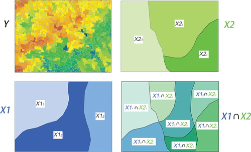
As more explanatory variables are introduced into any analysis, consideration needs to be given as to how the variables interact to affect the outcome (Y). In the case of two explanatory variables, X1 and X2, we can construct maps that reflect the underlying interaction between them (X1 ∩ X2) as illustrated in Figure 8. The interactions include, but are not limited to, the product interaction association studied in econometrics (Gujarati and Porter 2009, 263, 287, 470). Further, by comparing the values of q(X1), q(X2), and q(X1∩X2), one can start to explore how the interaction between X1 and X2 might be associated with linear or nonlinear variation in the level of Y. Luo et al. (2016) examined the interaction between determinants of landscape fragmentation in the United States. B. Xu et al. (2021) investigated the general interaction between meteorological indicators and the prevalence of respiratory viruses in China.

Figure 8. The general interaction between explanatory variables X1 and X2 impacting on a response variable Y: q(Y|X1$\cap$X2).

Spatial Goodness of Fit

Yin et al. (2019) developed a new indicator, maximum frequent temperature (MFT), to explain the minimum mortality temperature (MMT) globally. The Pearson coefficient between MMT and MFT is much larger than that between MMT and two other widely adopted indicators (Table 2). Additionally, q values are calculated with a suggestion that MFT matches to MMT, spatially, better than the remaining variables considered. Both statistics recommend the use of MFT to explain MMT.

Table 2. Statistical indexes between three temperature indicators and minimum mortality temperature (Yin et al. 2019)

	Annual mean temperature	78th percentile temperature	MFT
Pearson correlation	0.71	0.75	0.93
q-statistic	0.56	0.57	0.87

Note: MFT = maximum frequent temperature.

Geodetector q +

q is easily integrated with other methods to enhance their capacities. Examples are q + Kriging to map soil pollutions (Yang et al. 2022); q + GWR to investigate drought (Ji et al. 2022); q + InSAR to identify ground deformation (Chen et al. 2022); q + Google Earth Engine to study land-use changes (Liu et al. 2021); q + SWAT to assess water conservation functions (Yu, Wang, and Liu 2020); q + BHM to model point of interest urban vibrancy (Z. Wang et al. 2022); and q + deep learning to mapping tree canopy (Guo et al. 2023). For more examples, please refer to www.geodetector.cn.

SSH Plot

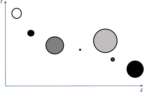
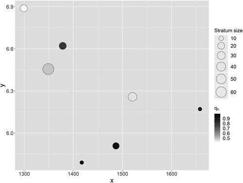
If X is a quantitative variable, then a bivariate plot of the means of X against the corresponding means of Y by strata will indicate the form of any association—which need not be linear. Note that for the two values of q(L; Px) with one calculated on Y and the other on X but with Px for both cases, an extension is required to determine which of the two variables is more homogeneous within the strata. Figure 9 decomposes the components of the q-function when the aim is to compare two variables (X and Y). We assume that the stratification of the map has been derived based on the spatial variation in the variable X (not Y). Each circle on the scatterplot refers to a single X-defined stratum. The center of any circle on the scatterplot is defined by the mean values of Y and X within that stratum, respectively. The size of any circle is proportional to the size of the stratum (in terms of population size or areal extent) to give visual weight to larger strata. However, the shading of any circle (for stratum h) is based on q_h = 1 – [σ_h²/σ²] calculated on the variable Y. The darker the shading, the smaller the within-stratum variance of Y (the within-stratum variance on X is small by construction) is. We are able to refine this plot further. If any stratum h comprises several discrete geographical areas (see Figure 4), then multiple circles for stratum h could be disaggregated with one for each discrete area. This might indicate that areas are large and widely scattered geographically. It might be undesirable to do this if each discrete geographical area is very small, thereby giving rise to the small number problem (see, e.g., Haining and Li 2020, 81).

Figure 9. q-function scatterplot. Arrows point in the direction of increasing values. Each circle refers to a single X-defined stratum. The size of any circle is proportional to the size of stratum. The shading of any circle is based on q_h = 1 - σ_h²/σ² calculated on Y, and the darker the shading the smaller the variance q_h. The scatterplot suggests, descriptively, a weak, inverse relationship between X and Y at the scale of seven aggregate strata of varying size. There might be a case for disaggregating the large circle, third from the right, if it comprises several discrete geographical areas. The same comment might apply to the two other larger circles—first from the right and third from the left.

Empirical Studies

In this section we review two empirical studies in geographical (or spatial) epidemiology where the presence of SSH raises methodological issues.

Obtaining a Map of Breast Cancer Incidence Using Sample Data: Comparing Sandwich and Kriging (China National Cancer Centre 2019)

Breast cancer mortality rates in the more than 2,700 counties of China in 1992 were collected from China’s Center for Disease Control (CDC; Figure 10A). Moran’s I test for spatial autocorrelation (using the four nearest counties as neighbors when specifying the W matrix) gave a value of 0.195 (p = 0.001). We calculated q for eight different partitions (L = 3, 4, … , 10 strata) of the breast cancer mortality data and the partition is based on selecting a large value of q while restricting the number of partitions (L). We chose the stratification (L = 5), which gave rise to the first significant value of q at the 1 percent level (q = 0.6381 with p < 0.01) while “penalizing” for increasing values of L (see Table 3). As we move from L = 4 to L = 5, q increases by 0.074 (from 0.564 to 0.638) and from a p value of 0.029 (not significant at the 1 percent level) to a p-value of 0.007 (significant at the 1 percent level). At the next level of stratification from L = 5 to L = 6, the improvement in L (which by definition must occur) is less than occurred when moving from four to five strata (0.061 compared to 0.074), indicating a decrease in the size of the improvement relative to the improvement when moving from L = 4 to L = 5. We are implicitly invoking a criterion of simplicity when trying to reach statistical significance of q with smaller L, a problem we will discuss again later. These two statistics (Moran’s I and the q-function) indicate that the breast cancer mortality data display both spatial autocorrelation and SSH at the county support.

Figure 10. Interpolation of (A) breast cancer mortality sample data using (B) spatially autocorrelated-based Kriging, and (C) spatially stratified heterogeneity–based sandwich methods.

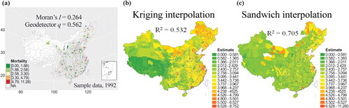
Table 3. q-function calculated for breast cancer mortality rates in China in 1992

	L
	3	4	5	6	7	8	9	10
q-function	0.400	0.564	0.638	0.699	0.733	0.774	0.818	0.823
p value	0.024	0.029	0.007	0.000	0.000	0.000	0.000	0.000

The SSH-based sandwich method used the mortality data from sixty-four sample counties (see Figure 10A) to construct a county-level map of breast cancer mortality for all the counties of China in 1992 (Figure 10C). The results obtained by this method and by Kriging (Figure 10B) were compared with the known mortality rates from the CDC database. The leave-one-out validation R² derived from sandwich mapping is 0.705, whereas for Kriging the value is 0.532. In this instance and therefore by the R² criterion, sandwich mapping outperforms Kriging. The mechanism behind the statistical findings could be that breast cancer (population) shows more SSH than SAC, perhaps reflecting SSH between urban and rural areas, epidemiologically. Therefore, an SSH-based estimator is theoretically more appropriate than an SAC-based estimator in this case. Aside from the many different reporting units that could have been presented derived from the original sample, the sandwich method has the particular merit of invoking simple modeling assumptions coupled with full utilization of the sample data through stratification rather than using only the nearest neighbor data values as in the case of Kriging. The evidence from this example indicates that the sandwich method performs well. It outperforms Kriging when the variable exhibits SSH. It clearly needs more work to determine whether this property holds more generally, particularly in the case when methods of Kriging, developed for heterogeneous surfaces, have been implemented.

Spatial Attribution of Neural Tube Defects in Heshun County

We summarize our findings from a pilot project investigating the factors associated with the geographical distribution of cases of neural tube defects (NTDs) in Heshun County, Shanxi Province (J. F. Wang, Li, et al. 2010). It is an area with one of the highest NTD incidence rates in China. The factors (X) believed to be responsible for variation in NTD incidence (Y) include the physical environment, man-made pollution, and nutrition. The factors (X) are measured at both a nominal level and a quantitative level and exhibit SSH (see Figure 11). The q-function (Figure 4) was used to examine the spatial association between NTD incidence and the suspected factors (x). The procedure for examining the association between a Y and any particular x is as follows. First, the map for the selected x is stratified to be Px. Second, the map for y is overlaid on the stratified map Px of the chosen x. Finally, the data on y are used to calculate q(L, Px). Software to calculate q is available at www.geodetector.cn.

Figure 11. (A) Example data of neural tube defect (NTD) incidence (Y) and suspected factors (X) (B) watershed, (C) soil type, and (D) elevation level. Source: Adapted from J. F. Wang, Li, et al. (2010).

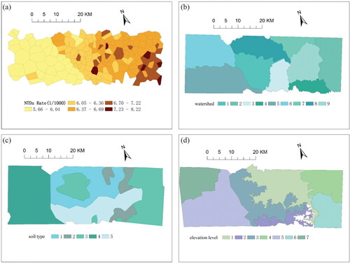
Figure 12 presents the q-function scatterplot between NTD incidence (Y) and elevation (X), a proxy for one of the suspected determinants. The scatterplot visualizes the SSH information of the data. For example, the rate of NTD incidence at elevation 1,300 m is high (6.9 percent) but very variable as indicated by the white color of the circle. Moreover, the stratum area to which these data refer is small (as indicated by the size of the circle). The four dark circles on the plot indicate elevations where NTD incidences are not highly variable but there is no evidence of a simple linear relationship between NTD incidence and elevation.

Figure 12. q-function scatterplot between neural tube defect incidence (Y) and elevation (X).

Table 4 presents the q-function between NTD incidence (Y) and three of the suspected determinants (Xs). The study found that some environmental factors (watershed type and elevation but not soil type) were found to be significantly associated with variation in NTD occurrence in the region. Usually water quality and the geological chemical environment are more similar within watersheds than between watersheds. Non-environmental factors (not reported here) were of secondary importance. These findings were helpful for identifying what courses of action would be most appropriate for disease intervention in the region (see J. F. Wang, Li, et al. 2010).

Table 4. q-function calculated for neural tube defect incidence using strata constructed for different suspected determinants

	Watershed	Elevation	Soil type
q-statistic	0.64	0.61	0.39
p value	0.00	0.04	0.36

In both of the examples and in several of the earlier sections, statistical results depend on the scale (size) of, or partitioning associated with, the reporting units (referred to as the MAUP; Openshaw 1984; Ge et al. 2019). This is an issue endemic within spatial analysis when working with areal units. Typically, the methods described here do not appear to give rise to any additional or significant scale effects because the reporting units themselves are unaffected (with the possible exception of some uses of the sandwich method where some source zones might be divided up and distributed over two or more target zones). The creation of homogenous subsets, however, adds another layer of the partition effect. This is why it is important to detect and justify the presence of spatial heterogeneity with the implementation of the corresponding methodology to identify homogeneous subsets as described earlier and discussed further next.

Discussion and Conclusions

SSH is prevalent when data cover a large geographical area or where the data are in high resolution. The problems caused by SSHy to statistics that assume homogeneity can be resolved or at least reduced if the structure of the heterogeneity can be identified, such that the map can be partitioned into homogeneous subpopulations. Conventional (iid) statistical methods can be used in each stratum if observations are independent, and spatial statistical methods should be used if the observations are SAC. If the structure of the SSH can be identified, then it can also be used to design sampling schemes that will help in drawing a representative sample that provides coverage of the different strata and reduces estimator bias.

Identifying SSH offers an opportunity for spatial interpolation when SAC is absent or weak. Besides providing a measure of SSH, the q-function can be used to explore the nonlinear association between the spatial patterns of two variables and has clear physical meaning, as was discussed earlier. Table 5 summarizes tools that are often used for data showing different states (presence–absence) of SSH and SAC.

Table 5. Examples of techniques when working with spatially stratified heterogeneous data

The statistical characteristics of geographical variables		Spatially stratified heterogeneity (SSH) (measured by q-function)
		Absent	Present
Spatial autocorrelation	Absent	Classical (iid) statistics	Spatial clustering methods, wombling, areal interpolation, sandwich estimation
	Present	Spatial statistics applied to identically distributed (id) data: Kriging, etc.	MSN (stratified sample), B-SHADE (biased sample), SPA (single-point sample), hierarchical modeling
			Causality inference for or by SSH

Note: MSN = means of surface with nonhomogeneity; B-SHADE = biased sentinel hospital area disease estimator; SPA = single-point area.

Although in certain research contexts SSH is endemic with numerous algorithms developed for spatial clustering, it has not received the attention that other special characteristics of spatial data have received. The development of statistics for SSH will add to the toolbox of exploratory spatial analysis techniques, alongside techniques for exploring data that are SAC (Anselin 1995).

Cressie (1993) remarked, “Whether one chooses to model the spatial variation through the (nonstochastic) mean structure (called large scale variation …) or the stochastic dependence structure (called small scale variation) depends on the underlying scientific problem, and can sometimes be simply a trade-off between model fit and parsimony in model description. What is one person’s (spatial) covariance structure may be another person’s mean structure” (25). This remark is relevant to the relationship between the characteristics of heterogeneity and spatial autocorrelation and how it might be handled in the course of data analysis (Atkinson and Tate 2000). For example, the behavior of local indicators of spatial association (LISA), Getis–Ord statistics, and GWR, all exploratory statistics, could be reflecting either local spatial autocorrelation (Anselin 1995; Sui 2006, 494) or spatial heterogeneity (Goodchild and Haining 2004; Anselin 2006). The semivariogram, well known in geostatistics, underpins Kriging. It is an interpolation method based on the spatial autocorrelation properties of a set of data. The method can also be employed to identify spatial heterogeneity (see Isaaks and Srivastava 1989, 223–24 and Figure 9.5; 292 and Figure 12.2 also discuss the use of the correlogram in Kriging). The two concepts, spatial heterogeneity and spatial autocorrelation, do not reflect distinct and separate features of spatial data. To paraphrase Cressie, “one person’s heterogeneity in the mean may be another person’s local or global spatial autocorrelation.” That said, one of the central points of this article has been to argue that SSH might, as in the examples presented here, fit better with the scientific problem and provide a satisfactory trade-off between model fit and model complexity.

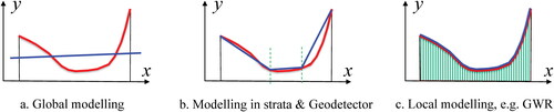
SSH offers an important opportunity for detection of spatial causality and for general interaction. When Y is nonmonotonically linked to X, modeling globally could be confounded (Christakos et al. 2017; Figures 2A and 13A), whereas a local model might be overfitting and neglects trends in the population (Figure 13C). Actually, a simple solution to the confounding is to partition the population into homogenous strata (Figure 13B), such that one can model the strata and regress the trends in strata, respectively, as suggested earlier. A further benefit from acknowledging SSH rises from the combining of the SSW and SST statistics as in the Geodetector q-function (Figure 4) so that the nonmonotonic association between two variables can be explored (Figure 13B), which could be missed by more conventional linear modeling.

Figure 13. Nonmonotonic population (red curve) and modeling strategies (blue lines). GWR = geographically weighted regression.

As a new tool to analyze SSH, we believe two issues related to the q-function need further investigation. First, the value of q(L, P) depends on both the number of strata and the spatial structure of the stratification. In some circumstances there could be a large number of plausible stratifications (in terms of both L and P) and efficient methods are needed to compare them. Closely related to this point, the decision on the number of strata to employ involves a trade-off between complexity (the number of strata) and the level of intrastratum homogeneity as discussed earlier. (How can we be sure that we have chosen the best L and P? Should it just be a statistical decision? How much substantive knowledge should be drawn on to make the final choice and how sensitive are our results to the chosen L and P?) In keeping with other forms of statistical decision-making, an AIC statistic could provide a way to formalize this trade-off, as suggested earlier, but more work is needed to assess this because AIC is not directly applicable. The reason is that the PDF that AIC is based on is not on a one-to-one mapping with the spatial distribution on which the q-function is based. For example, different spatial distributions (stratifications) might share the same PDF. Second, although spatial autocorrelation and SSH are two important characteristics of spatial data, the relationships between them and the influence of one on the other in the conduct of spatial data analysis need further investigation. Notwithstanding these concerns, there are a few rules of thumb that should be helpful in choosing (L, P) as we illustrated in this article.

Disclosure Statement

No potential conflict of interest was reported by the authors.

Correction Statement

This article has been corrected with minor changes. These changes do not impact the academic content of the article.

Additional information

Funding

This study was supported by the National Natural Science Foundation of China (No. 42071375, 41531179), Ministry of Science and Technology of China (2022YFC3600800; 2023YFF1305403), and the National Social Science Foundation of China (No. 21&ZD186).

Notes on contributors

Jinfeng Wang

JINFENG WANG is a Professor in the State Key Laboratory of Resources and Environmental Information System, Institute of Geographic Sciences and Natural Resources Research, Chinese Academy of Sciences, Beijing, China, and in the University of Chinese Academy of Sciences, Beijing, China. E-mail: [email protected]. His primary research interest is methodologies for spatial sampling and statistical inference with applications in health research.

Robert Haining

ROBERT HAINING is Emeritus Professor in the Department of Geography at the University of Cambridge, Cambridge CB2 3EN, UK. E-mail: [email protected]. His primary research interest is the methodologies for spatial data analysis with applications in health services research and the geography of crime.

Tonglin Zhang

TONGLIN ZHANG is an Associate Professor in the Department of Statistics, Purdue University, Lafayette, IN 47907, USA. E-mail: [email protected]. His research interests are the methodologies for mathematical statistics and spatial epidemiology.

Chengdong Xu

CHENGDONG XU is an Associate Professor in the State Key Laboratory of Resources and Environmental Information System, Institute of Geographic Sciences and Natural Resources Research, Chinese Academy of Sciences, Beijing, China. E-mail: [email protected]. His research interest is GIScience.

Maogui Hu

MAOGUI HU is an Associate Professor in the State Key Laboratory of Resources and Environmental Information System, Institute of Geographic Sciences and Natural Resources Research, Chinese Academy of Sciences, Beijing, China. E-mail: [email protected]. His primary research interest is spatial statistics with applications in health research.

Qian Yin

QIAN YIN is an Associate Professor in the State Key Laboratory of Resources and Environmental Information System, Institute of Geographic Sciences and Natural Resources Research, Chinese Academy of Sciences, Beijing, China. E-mail: [email protected]. Her primary research interest is spatial epidemiology.

Lianfa Li

LIANFA LI is a Professor in the State Key Laboratory of Resources and Environmental Information System, Institute of Geographic Sciences and Natural Resources Research, Chinese Academy of Sciences, Beijing, China. E-mail: [email protected]. His primary research interest is methodologies for spatial machine learning and artificial intelligence.

Chenghu Zhou

CHENGHU ZHOU is a Professor in the State Key Laboratory of Resources and Environmental Information System, Institute of Geographic Sciences and Natural Resources Research, Chinese Academy of Sciences, Beijing, China; and a Professor in the University of Chinese Academy of Sciences, Beijing, China. E-mail: [email protected]. His primary research interest is GIScience.

Guangquan Li

GUANGQUAN LI is an Assistant Professor in the Department of Mathematics, Physics and Electrical Engineering at the Northumbria University, Newcastle upon Tyne NE1 8ST, UK. E-mail: [email protected]. His primary research interest is Bayesian methodologies to analyze data arising from health and social sciences.

Hongyan Chen

HONGYAN CHEN is a spatial data scientist in the UK Centre for Ecology & Hydrology, Lancaster Environment Centre, Lancaster, LA1 4AP, UK. E-mail: [email protected]. Her primary research interest is GIScience.

References

- Akaike, H. 1974. A new look at the statistical model identification. IEEE Transactions on Automatic Control 19 (6):716–23. doi: 10.1109/TAC.1974.1100705.
- Anselin, L. 1995. Local indicators of spatial association—LISA. Geographical Analysis 27 (2):93–115. doi: 10.1111/j.1538-4632.1995.tb00338.x.
- Anselin, L. 2006. Spatial heterogeneity. In Encyclopedia of human geography, ed. B. Warff, 452–53. Thousand Oaks, CA: Sage.
- Atkinson, P., and N. Tate. 2000. Spatial scale problems and geostatistical solutions: A review. The Professional Geographer 52 (4):607–23. doi: 10.1111/0033-0124.00250.
- Bradley, V. C., S. Kuriwaki, M. Isakov, D. Sejdinovic, X. L. Meng, and S. Flaxman. 2021. Unrepresentative big surveys significantly overestimated US vaccine uptake. Nature 600 (7890):695–700. doi: 10.1038/s41586-021-04198-4.
- Buttle, J. M., D. M. Allen, D. Caissie, B. Davison, M. Hayashi, D. L. Peters, J. W. Pomeroy, S. Simonovic, A. St-Hilair, and P. H. Whitfield. 2016. Flood processes in Canada: Regional and special aspects. Canadian Water Resources Journal 41 (1–2):7–30. doi: 10.1080/07011784.2015.1131629.
- Chen, J., T. Wu, D. Zou, L. Liu, X. Wu, W. Gong, X. Zhu, R. Li, J. Hao, G. Hu, et al. 2022. Magnitudes and patterns of large-scale permafrost ground deformation revealed by Sentinel-1 InSAR on the central Qinghai-Tibet Plateau. Remote Sensing of Environment 268:112778. doi: 10.1016/j.rse.2021.112778.
- China National Cancer Centre. 2019. Cancer atlas in China. Beijing: Sinomap Press.
- Christakos, G. 1992. Random field models in earth sciences. San Diego, CA: Academic Press.
- Christakos, G. 2012. Modern spatiotemporal geostatistics. New ed. Mineola, NY: Dover.
- Christakos, G., J. M. Angulo, H.-L. Yu, and J. P. Wu. 2017. Space–time metric determination in environmental modeling. Journal of Environmental 30 (1):29–40.
- Cliff, A. D., and J. K. Ord. 1981. Spatial processes: Models and application. London: Pion.
- Cressie, N. 1993. Statistics for spatial data. New York: Wiley.
- Dunn, R., and A. R. Harrison. 1993. Two dimensional systematic sampling of land use. Applied Statistics 42 (4):585–601. doi: 10.2307/2986177.
- Dutilleul, P. R. L. 2011. Spatio-temporal heterogeneity: Concepts and analysis. Cambridge, UK: Cambridge University Press.
- Einstein, A. 1953. Einstein Archive, 61–381. Accessed December 17, 2023. http://www.autodidactproject.org/quote/einstn2.html.
- Everitt, B. S., and A. Skrondal. 2010. The Cambridge dictionary of statistics. 4th ed. Cambridge, UK: Cambridge University Press.
- Fotheringham, A. S., C. Brunsdon, and M. Charlton. 2000. Quantitative geography: Perspectives on spatial data analysis. London: Sage.
- Gao, B.-B., J.-F. Wang, H.-M. Fan, K. Xu, M.-G. Hu, and Z.-Y. Chen. 2015. A stratified optimization method for a multivariate marine environmental monitoring network in the Yangtze River estuary and its adjacent sea. International Journal of Geographical Information Science 29 (8):1332–49. doi: 10.1080/13658816.2015.1024254.
- Gao, B. B., J. Y. Yang, Z. Y. Chen, G. Sugihara, M. C. Li, A. Stein, M. B. Kwan, and J. F. Wang. 2023. Causal inference from cross-sectional earth system data with geographical convergent cross mapping. Nature Communications 14 (1):5875. doi: 10.1038/s41467-023-41619-6.
- Ge, Y., Y. Jin, A. Stein, Y. Chen, J. Wang, J. Wang, Q. Cheng, H. Bai, M. Liu, and P. M. Atkinson. 2019. Principles and methods of scaling geospatial earth science data. Earth-Science Reviews 197:102897. doi: 10.1016/j.earscirev.2019.102897.
- Getis, A., and J. K. Ord. 1992. The analysis of spatial association by use of distance statistics. Geographical Analysis 24 (3):189–206. doi: 10.1111/j.1538-4632.1992.tb00261.x.
- Goldstein, H. 2011. Multilevel statistical models. 4th ed. Chichester, UK: Wiley.
- Goodchild, M. F., L. Anselin, and U. Deichmann. 1993. A framework for the areal interpolation of socioeconomic data. Environment and Planning A: Economy and Space 25 (3):383–97. doi: 10.1068/a250383.
- Goodchild, M., and R. Haining. 2004. GIS and spatial data analysis: Converging perspectives. Papers in Regional Science 83 (1):363–85. doi: 10.1007/s10110-003-0190-y.
- Griffith, D. A. 2003. Spatial autocorrelation and spatial filtering, gaining understanding through theory and visualization. Berlin: Springer-Verlag.
- Gujarati, D. N., and D. C. Porter. 2009. Basic econometrics. 5th ed. New York: McGraw-Hill.
- Guo, J. H., Q. S. Xu, Y. Zeng, Z. H. Liu, and X. X. Zhu. 2023. Nationwide urban tree canopy mapping and coverage assessment in Brazil from high-resolution remote sensing images using deep learning. ISPRS Journal of Photogrammetry and Remote Sensing 198:1–15. doi: 10.1016/j.isprsjprs.2023.02.007.
- Haining, R. 2003. Spatial data analysis: Theory and practice. Cambridge, UK: Cambridge University Press.
- Haining, R., and G. Q. Li. 2020. Modelling spatial and spatial-temporal data: A Bayesian approach. Boca Raton, FL: CRC.
- Heckman, J. J. 1979. Sample selection bias as a specification error. Econometrica 47 (1):153–61. doi: 10.2307/1912352.
- Hox, J. J. 2010. Multilevel analysis: Techniques and applications. 2nd ed. London and New York: Routledge.
- Hu, M. G., and J. F. Wang. 2011. A meteorological network optimization package using MSN theory. Environmental Modelling & Software 26 (4):546–48. doi: 10.1016/j.envsoft.2010.10.006.
- Hu, M.-G., J.-F. Wang, Y. Zhao, and L. Jia. 2013. A B-SHADE based best linear unbiased estimation tool for biased samples. Environmental Modelling & Software 48:93–97. doi: 10.1016/j.envsoft.2013.06.011.
- Imbens, G. W., and D. B. Rubin. 2015. Causal inference in statistics, social, and biomedical science. Cambridge, UK: Cambridge University Press.
- Isaaks, E., and R. Srivastava. 1989. Applied geostatistics. New York: Oxford University Press.
- Ji, B. W., Y. B. Qin, T. B. Zhang, X. B. Zhou, G. H. Yi, M. T. Zhang, and M. L. Li. 2022. Analyzing driving factors of drought in growing season in Inner Mongolia based on Geodetector and GWR models. Remote Sensing 14 (23):6007. doi: 10.3390/rs14236007.
- Kulldorff, M. 1997. A spatial scan statistic. Communications in Statistics: Theory and Methods 26 (6):1481–96. doi: 10.1080/03610929708831995.
- Li, X., M. Feng, Y. Ran, Y. Su, F. Liu, C. Huang, H. Shen, Q. Xiao, J. Su, S. Yuan, et al. 2023. Big data in Earth system science and progress towards a digital twin. Nature Reviews Earth & Environment 4 (5):319–32. doi: 10.1038/s43017-023-00409-w.
- Lin, Y., C. D. Xu, and J. F. Wang. 2023. Sandwichr: Spatial prediction in R based on spatial stratified heterogeneity. Transactions in GIS 27 (5):1579–98. doi: 10.1111/tgis.13088.
- Lindley, D. V., and M. R. Novick. 1981. The role of exchangeability in inference. Annals of Statistics 9:45–58.
- Liu, C., W. Li, W. Wang, H. Zhou, T. Liang, F. Hou, J. Xu, and P. Xue. 2021. Quantitative spatial analysis of vegetation dynamics and potential driving factors in a typical alpine region on the northeastern Tibetan Plateau using the Google Earth Engine. Catena 206:105500. doi: 10.1016/j.catena.2021.105500.
- Lloyd, C. D. 2010. Local models for spatial analysis. 2nd ed. Boca Raton, FL: CRC.
- Longley, P. A., M. F. Goodchild, D. J. Maguire, and D. W. Rind. 2005. Geographical information systems and science. 2nd ed. Hoboken, NJ: Wiley.
- Luo, W., J. Jasiewicz, T. Stepinski, J. Wang, C. Xu, and X. Cang. 2016. Spatial association between dissection density and environmental factors over the entire conterminous United States. Geophysical Research Letters 43 (2):692–700. doi: 10.1002/2015GL066941.
- Matheron, G. 1963. Principles of geostatistics. Economic Geology 58 (8):1246–66. doi: 10.2113/gsecongeo.58.8.1246.
- Meng, X. L. 2018. Statistical paradises and paradoxes in big data (I): Law of large populations, big data paradox, and the 2016 US presidential election. The Annals of Applied Statistics 12 (2):685–726. doi: 10.1214/18-AOAS1161SF.
- Moran, P. 1950. Notes on continuous stochastic phenomena. Biometrika 37 (1–2):17–23.
- O’Connell, P. E., R. J. Gurney, D. A. Jones, J. B. Miller, C. A. Nicholass, and M. R. Senior. 1979. A case study of rationalization of a rain gauge network in SW England. Water Resources Research 15 (6):1813–22. doi: 10.1029/WR015i006p01813.
- Openshaw, S. 1984. The modifiable areal unit problem: CATMOG 38. Norwich, UK: GeoAbstracts
- Pearl, J., and D. Mackenzie. 2018. The book of why: The new science of cause and effect. New York: Basic Books.
- Pearson, K. 1895. Notes on regression and inheritance in the case of two parents. Proceedings of the Royal Society of London 58:240–42.
- Rao, J. N. K. 2003. Small area estimation. New York: Wiley.
- Ripley, B. D. 1981. Spatial statistics. New York: Wiley.
- Rodríguez-Iturbe, I., and J. M. Mejía. 1974. The design of rainfall networks in time and space. Water Resources Research 10 (4):713–28. doi: 10.1029/WR010i004p00713.
- Runge, J., A. Gerhardus, G. Varando, V. Eyring, and G. Camps-Valls. 2023. Causal inference for time series. Nature Reviews Earth & Environment 4 (7):487–505. doi: 10.1038/s43017-023-00431-y.
- Snijders, T. A. B., and R. J. Bosker. 2011. Multilevel analysis: An introduction to basic and advanced multilevel modeling. 2nd ed. Thousand Oaks, CA: Sage.
- Snow, J. 1854. On the mode of communication of cholera. London, Churchill.
- Stein, A. 2022. The development of the journal Spatial Statistics: The first 10 years. Spatial Statistics 50:100576. doi: 10.1016/j.spasta.2021.100576.
- Stein, A., M. Hoogerwerf, and J. Bouma. 1988. Use of soil-map delineations to improve (Co-)kriging of point data on moisture deficits. Geoderma 43 (2–3):163–77. doi: 10.1016/0016-7061(88)90041-9.
- Sugihara, G., R. Ma, H. Ye, C. Hsieh, E. Deyle, M. Fogarty, and S. Munch. 2012. Detecting causality in complex ecosystems. Science 338 (6106):496–500. doi: 10.1126/science.1227079.
- Sui, D. 2006. Tobler’s first law of geography. In Encyclopedia of human geography, ed. B. Warff, 454. Thousand Oaks, CA: Sage.
- Wang, J. F., G. Christakos, and M. G. Hu. 2009. Modeling spatial means of surfaces with stratified non-homogeneity. IEEE Transactions on Geoscience and Remote Sensing 47 (12):4167–74. doi: 10.1109/TGRS.2009.2023326.
- Wang, J. F., R. Haining, and Z. D. Cao. 2010. Sample surveying to estimate the mean of a heterogeneous surface: Reducing the error variance through zoning. International Journal of Geographical Information Science 24 (4):523–43. doi: 10.1080/13658810902873512.
- Wang, J.-F., R. Haining, T.-J. Liu, L.-F. Li, and C.-S. Jiang. 2013. Sandwich estimation for multi-unit reporting on a stratified heterogeneous surface. Environment and Planning A: Economy and Space 45 (10):2515–34. doi: 10.1068/a44710.
- Wang, J. F., M. G. Hu, C. D. Xu, G. Christakos, and Y. Zhao. 2013. Estimation of citywide air pollution in Beijing. PloS ONE 8 (1):e53400. doi: 10.1371/journal.pone.0053400.
- Wang, J. F., X. H. Li, G. Christakos, Y. L. Liao, T. Zhang, X. Gu, and X. Y. Zheng. 2010. Geographical detectors-based health risk assessment and its application in the neural tube defects study of the Heshun Region, China. International Journal of Geographical Information Science 24 (1):107–27. doi: 10.1080/13658810802443457.
- Wang, J.-F., B. Y. Reis, M.-G. Hu, G. Christakos, W.-Z. Yang, Q. Sun, Z.-J. Li, X.-Z. Li, S.-J. Lai, H.-Y. Chen, et al. 2011. Area disease estimation based on sentinel hospital records. PLoS ONE 6 (8):e23428. doi: 10.1371/journal.pone.0023428.
- Wang, J., C. Xu, M. Hu, Q. Li, Z. Yan, and P. Jones. 2018. Global land surface air temperature dynamics since 1880. International Journal of Climatology 38 (Suppl. 1):e466–e474. doi: 10.1002/joc.5384.
- Wang, J. F., T. L. Zhang, and B. J. Fu. 2016. A measure of spatial stratified heterogeneity. Ecological Indicators 67:250–56. doi: 10.1016/j.ecolind.2016.02.052.
- Wang, Z., F. Lu, Z. Liu, W. Tu, K. Nie, Q. Du, Q. Li, and Z. Wu. 2022. Measuring spatial nonstationary effects of POI-based mixed use on urban vibrancy using Bayesian spatially varying coefficients model. International Journal of Geographical Information Science 37 (2):339–59. doi: 10.1080/13658816.2022.2117363.
- Womble, W. H. 1951. Differential systematics. Science 114 (2961):315–22. doi: 10.1126/science.114.2961.315.
- Worobey, M., J. I. Levy, L. Malpica Serrano, A. Crits-Christoph, J. E. Pekar, S. A. Goldstein, A. L. Rasmussen, M. U. G. Kraemer, C. Newman, M. P. G. Koopmans, et al. 2022. The Huanan seafood wholesale market in Wuhan was the early epicenter of the COVID-19 pandemic. Science 377 (6609):951–59. doi: 10.1126/science.abp8715.
- Xu, B., J. Wang, Z. Li, C. Xu, Y. Liao, M. Hu, J. Yang, S. Lai, L. Wang, and W. Yang. 2021. Seasonal association between viral causes of hospitalised acute lower respiratory infections and meteorological factors in China: A retrospective study. The Lancet: Planetary Health 5 (3):e154–e163. doi: 10.1016/S2542-5196(20)30297-7.
- Xu, C., J. Wang, M. Hu, and W. Wang. 2022. A new method for interpolation of missing air quality data at monitor stations. Environment International 169:107538. doi: 10.1016/j.envint.2022.107538.
- Xu, C. D., J. F. Wang, and Q. X. Li. 2018. A new method for temperatures spatial interpolation based on sparse historical stations. Journal of Climate 31 (5):1757–70. doi: 10.1175/JCLI-D-17-0150.1.
- Xu, L., Q. Liu, L. C. Stige, T. Ben Ari, X. Fang, K.-S. Chan, S. Wang, N. C. Stenseth, and Z. Zhang. 2011. Nonlinear effect of climate on plague during the third pandemic in China. Proceedings of the National Academy of Sciences of the United States of America 108 (25):10214–19. doi: 10.1073/pnas.1019486108.
- Yang, J., J. Wang, X. Liao, H. Tao, and Y. Li. 2022. Chain modeling for the biogeochemical nexus of cadmium in soil–rice–human health system. Environment International 167:107424. doi: 10.1016/j.envint.2022.107424.
- Yin, Q., J. Wang, Z. Ren, J. Li, and Y. Guo. 2019. Mapping the increased minimum mortality temperatures in the context of global climate change. Nature Communications 10 (1):4640. doi: 10.1038/s41467-019-12663-y.
- Yu, C. L., Z. C. Wang, and D. Liu. 2020. Evolution process and driving force analysis of natural wetlands in Xiliao River Basin based on SWAT mode. Transactions of the Chinese Society of Agricultural Engineering 36 (22):286–97.
- Zhang, D. D., P. Brecke, H. F. Lee, Y.-Q. He, and J. Zhang. 2007. Global climate change, war, and population decline in recent human history. Proceedings of the National Academy of Sciences of the United States of America 104 (49):19214–19. doi: 10.1073/pnas.0703073104.