Development of graphical user interface for design of experiments via Gaussian process regression and its case study

ABSTRACT

Bayesian optimization, coupled with Gaussian process regression and acquisition functions, has proven to be a powerful tool in the field of experimental design. Nevertheless, it demands a profound proficiency in software programming, machine learning, and statistical concepts. This steep learning curve presents a substantial obstacle when implementing Bayesian optimization for experimental design. In order to overcome this challenge, a user-friendly graphical interface for Gaussian process regression and acquisition functions is proposed. This accessible tool can be readily accessed via web browsers, courtesy of the established CADS platform (available at https://cads.eng.hokudai.ac.jp/). Thus, the interface offers to perform Bayesian optimization without any programming or any extensive prior knowledge about Bayesian optimization and machine learning.

GRAPHICAL ABSTRACT

IMPACT STATEMENT

A user-friendly graphical interface for Bayesian optimization with Gaussian process　regression and acquisition functions is proposed. The interface offers to perform Bayesian optimization without any programming or any extensive prior knowledge about Bayesian optimization and machine learning.

KEYWORDS:

• Machine learning
• graphical user interface
• Bayesian optimization

1. Introduction

With the rise of materials and catalysts informatics, there is a notable increase in the utilization of data science in material science where machine learning has garnered significant attention [1–3]. The fundamental concept of machine learning revolves around establishing connections between materials properties and their corresponding descriptor variables, which may contain experimental conditions and compositions [4–7]. In general, variables responsible for representing properties are defined as descriptors or features while properties that the user wants to predict are defined as target variables. Among the machine learning, Gaussian process regression has emerged as a viable alternative for the design of experiments [8–10]. In general, orthogonal arrays are employed in experimental design to systematically test all conceivable combinations of experimental conditions in an efficient manner. Despite the potency of the design of experiments, it does not guarantee the attainment of optimal conditions. Such circumstance, Bayesian optimization combining with Gaussian process regression and acquisition function has garnered significant interest. The idea of the method is that, machine learning regression model fit the train data where standard deviation is also calculated. Through the use of the acquisition function, the approach identifies the optimal data points characterized by either high or low values predicted by the machine learning model, coupled with elevated uncertainty denoted by a high standard deviation. By continually updating the training data, this methodology aims to expedite the discovery of optimal data points compared to traditional design of experiments.

Although Bayesian optimization combining with Gaussian process regression and acquisition function is proposed to be a powerful approach, it has a major drawback. Specifically, the process requires the high level of programming skillset, deep knowledge of machine learning and statistics. This restricts the experimental researchers to implement the method. These types of issues are quite common in materials informatics. In order to overcome the drawback, graphical user interface is required where the user can perform materials informatics tool without the use of programming and machine learning knowledge [1]. Catalyst Acquisition by Data Science (CADS), https://cads.eng.hokudai.ac.jp/, has been developed previously [11]. CADS offers the various data science techniques such as machine learning, scientific visualization, and even image processing. Here, Bayesian optimization for the design of experiment is developed for CADS.

2. CADS analysis and visualization components

2.1. Architecture

The architecture of Catalyst Acquisition by Data Science (CADS) is illustrated in Figure 1. This depiction showcases CADS as comprising both client-side and server-side components. On the server side, it encompasses core programming codes responsible for executing tasks such as machine learning, data visualization, data management, and image processing. These integral codes are scripted in Python, utilizing libraries such as Django, scikit-learn, scikit-image, and pandas. Consequently, all data analyses are conducted at the server level. Conversely, the client side furnishes a graphical user interface that facilitates user interactions and displays responses originating from the server side. Users access CADS through a web browser. Within this architecture, users engage with the client side via their preferred web browser. They select their desired data analysis tools and submit inputs accordingly. Subsequently, these inputs are transmitted to the server side for further data analysis, with the outcomes subsequently returned to the client side. This framework empowers users to execute data analyses without requiring proficiency in any programming language. In the case of uploading the data, input data format is set to csv. The maximum file size is limited to 10 Mb. CSV file has to contain descriptors and objective variables that the users like to test.

Figure 1. Architecture of CADS.

With CADS architecture, Gaussian process regression within scikit learn and acquisition function are implemented in server side while graphical user interface of them is also designed and developed. At server side, Gaussian process regression is implemented. Here, the kernels below are introduced as a kernel choice.

• ConstantKernel() × RBF() + WhiteKernel()

• ConstantKernel() × DotProduct() + WhiteKernel()

• ConstantKernel() × RBF() + WhiteKernel() + ConstantKernel() × DotProduct()

• ConstantKernel() × RBF(np.ones(number_features)) + WhiteKernel()

• ConstantKernel() × RBF(np.ones(number_features)) + WhiteKernel() + ConstantKernel() × DotProduct()

Note that number features represents the count of variables within descriptor variables.

Gaussian regression model fit the train data where standard deviation is also calculated. Here, a large standard deviation value means the data point is far from the trained data. Through the use of the acquisition function represented by either Equations (1(1) $U=\frac{y_{max}+\mu -\xi }{\sigma }$(1) –3(3) $EI=\sigma \times U\times \mathrm{\Phi }(U)+\sigma \times \varphi (U)$(3) ), the approach identifies the optimal data points characterized by either high or low values predicted by Gaussian regression model, coupled with elevated uncertainty denoted by a high standard deviation. The acquisition function is calculated using Equations (1)(1) $U=\frac{y_{max}+\mu -\xi }{\sigma }$(1) and (2(2) $U=\frac{y_{min}-\mu -\xi }{\sigma }$(2) ) for maximization and minimization, respectively, where expected improvement is calculated by Equation (3)(3) $EI=\sigma \times U\times \mathrm{\Phi }(U)+\sigma \times \varphi (U)$(3) .

(1) $U=\frac{y_{max}+\mu -\xi }{\sigma }$(1)

(2) $U=\frac{y_{min}-\mu -\xi }{\sigma }$(2)

(3) $EI=\sigma \times U\times \mathrm{\Phi }(U)+\sigma \times \varphi (U)$(3)

Note that ${\mathrm{y}}_{\mathrm{m}\mathrm{a}\mathrm{x}}$ (${\mathrm{y}}_{\mathrm{m}\mathrm{i}\mathrm{n}}$) is the highest (lowest) target variable in the trained data set, $\xi$ is the optimization parameter calculated from the standard deviation of the predicted variables multiplied by 0.01, $\mu$ and $\sigma$ are predicted target variable and standard deviation calculated by Gaussian process regression, respectively, and $\mathrm{\Phi }(U)$ and $\varphi (U)$ are the cumulative distribution function and probability density function of U in Equations (1)(1) $U=\frac{y_{max}+\mu -\xi }{\sigma }$(1) or (2(2) $U=\frac{y_{min}-\mu -\xi }{\sigma }$(2) ), respectively.

Here, the graphical user interface of Gaussian process is shown in Figure 2. Figure 2 demonstrates that the user can select the number of feature columns, target variable, and features variables by just clicking.

Figure 2. Graphical user interface of Gaussian process regression.

Min and Max represent the range in which the user wants the machine to make predictions. Meanwhile, Number of Division represents how many divisions the machine divides that range into, thereby allowing the user to control how detailed or accurate the predictions may be. The maximum number of divisions that the machine can consider is 500. The user must also choose whether the user wants to see the maximization or minimization based on Equations (1)(1) $U=\frac{y_{max}+\mu -\xi }{\sigma }$(1) and (2(2) $U=\frac{y_{min}-\mu -\xi }{\sigma }$(2) ), respectively. A larger EI points to optimal experimental conditions for maximizing or minimizing the data. This user-selectable choice allows for adaptation to the specific nature of the data, whether it requires maximization or minimization. In addition, five kernels within Gaussian process regression can also be chosen. It also has a button called ‘Get Score’ which returns R² score from cross-validation where data set is randomly split to 20% test and 80% train data. Lastly, the user can choose the result of the Gaussian process. ‘Prediction’ visualizes the predicted target variables against feature variables predicted by Gaussian process regression. ‘Standard deviation’ option visualizes the standard deviation calculated by Gaussian process regression. ‘Expected improvement’ returns as expected improvement calculated by predicted target variables and standard deviation based on acquisition function where it also visualizes the result. ‘Prediction’, ‘Standard deviation’, and ‘Expected Improvement’ are represented graphically as visualizations, and ‘Proposed experimental conditions’, comprising the top 10 EI, is presented in tabular format along with their respective descriptor variable. Note that users must be careful regarding top EI where similar experimental conditions may be present within the top 10 EI, depending on the specifics of the division selected by the user. Thus, the user must exert caution with the exploration process and pay attention to whether predictions are performed within narrow or large exploratory spaces.

The workflow details of the process shown in Figure 3 are further explored. Here, the train data have a feature variable between 1 and 8 and corresponding target variables are displayed in Figure 3. In order to set up the Gaussian Process View, one must first understand what column in the data is the target column and what column(s) are the features related to it. In a simple case of columns x and y, x is defined as a feature column and y is defined as the target column. In this case, the minimum and maximum of x are defined. These points represent the range that the Gaussian model should focus on when it makes its prediction after training on the data. For this view, each feature column must have a minimum and maximum defined before the View can properly be run. Additionally, in the example shown in Figure 3, the number of divisions is set to 100, meaning that the machine will break down the defined range of 3 to 6 into 100 elements. With the target column, one must then decide whether they are interested in maximization or minimization for target variable. For this example, minimization is selected. A kernel must then be defined. The View provides the user five different kernels to choose from where the user can explore the optimal kernels. The kernel ‘ConstantKernel()$\times$RBF()+WhiteKernel()’ is chosen. Lastly, the user can decide what type of information the View should provide once the Gaussian model trains on the data. In this example, the Gaussian Process View is being set up to determine which areas can be targeted for consequent experiments and investigations; thus, ‘Expected Improvement’ is selected. ‘Proposed experimental conditions’ is a good companion to this option as it shows the results as a table, and is recommended for use within a different view to compare against each other. Here, it shows that expected improvement between 4.5 and 5 has large expected improvement; thus, those variables have a potential to minimize the target variable. Thus, Bayesian optimization is performed without any programming language.

Figure 3. General work from Bayesian optimization in CADs.

On the front end of the Gaussian process component, there is a configuration form, which allows the gathering of setup information from the user on how to manage and display the input data. When the user submits those settings, it is packaged properly in JSON format and sent to the Python server and the Gaussian process manager on the back end. The back end will then begin the machine learning calculations, utilizing the power of the scikit-learn library together with numpy and pandas and, while doing so, let the front end inform the user to stand by and wait. When all is done on the server, the end result is returned to the client-side front end as promised, and it is then forwarded to the rendering part of the component that will read the data and any additional settings in order to draw out the proper visualization using the Plotly.JS library. Depending on how many features are added, it will also control the visualization. If only one feature plus the target column is added, the visualization will be shown using a standard 2D plot, and if two features and the target features are present, then the visualization will use a 3D plot. For all other number of features (three and above), the visualization will be done with parallel coordinates.

3. Case studies

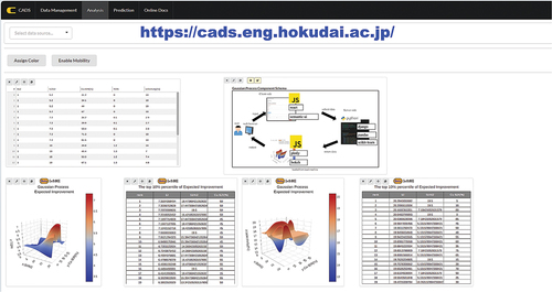
Bayesian optimization using the created graphical user interface is performed using chemical reaction data. Here, direct methanol synthesis from methane using Cu-zeolite is performed based on the previous work [10]. The results are demonstrated in Figure 4. In Figure 4, that trained data are displayed via CADS built in table. Then, the developed graphical user interface that shows the results of Bayesian optimization is demonstrated below the table. Si/Al ratio and Cu exchange rate are descriptors variable while selectivity and turnover number (TON) are individually selected as an objective variable. Here, expected improvement (EI) calculated by acquisition function is displayed against Si/Al ratio and Cu exchange rate for selectivity and TON. Both 3D plots indicate that high EI points, thus, user can easily identify the potential Si/Al ratio and Cu exchange rate. The results have a good agreement with previous work [10].

Figure 4. Case study: methanol synthesis from methane for maximizing selectivity and turnover number (TON). Si/Al ratio and Cu exchange rate are set as descriptor variables.

4. Conclusion

In conclusion, a web-based graphic user interface of the Bayesian optimization, Gaussian process regression, and acquisition functions is developed within CADS platform (https://cads.eng.hokudai.ac.jp/). It offers a viable alternative for experiment design without proficiency in programming languages, machine learning, and statistics. This initiative aims to democratize the application of Bayesian optimization, making it more accessible and practical for a wider range of users.

5. Code

The complete source code for the Gaussian Process component can be found together with the public source code (Under MIT licence) for the whole CADS system on GitHub at the following web address: https://github.com/Material-MADS/mads-app.

Disclosure statement

No potential conflict of interest was reported by the author(s).

Additional information

Funding

This work is funded by Japan Science and Technology Agency(JST) CREST Grant Number [JPMJCR17P2], ERATO grant number [JPMJER1903], JST Mirai Program Grant Number [JPMJMI22G4], JSPS KAKENHI Grant-in-Aid for Scientific Research (B) Grant Number [JP23H01762].

References

- Jain A, Ong SP, Hautier G, et al. Commentary: the materials project: a materials genome approach to accelerating materials innovation. APL Mater. 2013;1. doi: 10.1063/1.4812323
- Takahashi K, Takahashi L. Toward the golden age of materials informatics: perspective and opportunities. J Phys Chem Lett. 2023;14(20):4726–6. doi: 10.1021/acs.jpclett.3c00648
- Taniike T, Takahashi K. The value of negative results in data-driven catalysis research. Nat Catal. 2023;6(2):108–111. doi: 10.1038/s41929-023-00920-9
- Ulissi ZW, Medford AJ, Bligaard T, et al. To address surface reaction network complexity using scaling relations machine learning and DFT calculations. Nat Commun. 2017;8(1):14621. doi: 10.1038/ncomms14621
- Medford AJ, Kunz MR, Ewing SM, et al. Extracting knowledge from data through catalysis informatics. ACS Catal. 2018;8(8):7403–7429. doi: 10.1021/acscatal.8b01708
- Ramprasad R, Batra R, Pilania G, et al. Machine learning in materials informatics: recent applications and prospects. Npj Comput Mater. 2017;3(1):54. doi: 10.1038/s41524-017-0056-5
- Takahashi K, Ohyama J, Nishimura S, et al. Catalysts informatics: paradigm shift towards data-driven catalyst design. Chem Comm. 2023;59(16):2222–2238. doi: 10.1039/D2CC05938J
- Frazier PI, Wang J. Information science for materials discovery and design. Switzerland: Cham, Springer International Publishing; 2015. p. 45–75.
- Shields BJ, Stevens J, Li J, et al. Bayesian reaction optimization as a tool for chemical synthesis. Nature. 2021;590(7844):89–96. doi: 10.1038/s41586-021-03213-y
- Ohyama J, Tsuchimura Y, Yoshida H, et al. Bayesian-optimization-based improvement of cu-CHA catalysts for direct partial oxidation of CH4. J Phys Chem C. 2022;126(46):19660–19666. doi: 10.1021/acs.jpcc.2c04229
- Fujima J, Tanaka Y, Miyazato I, et al. Catalyst acquisition by data science (CADS): a web-based catalyst informatics platform for discovering catalysts. React Chem Eng. 2020;5(5):903–911. doi: 10.1039/D0RE00098A