Feature extraction and spatial imaging of synchrotron radiation X-ray diffraction patterns using unsupervised machine learning

ABSTRACT

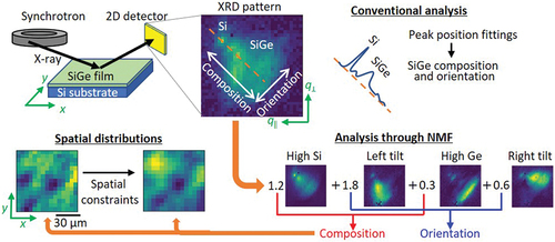
We analyzed a number of complicated X-ray diffraction patterns using feature patterns obtained through unsupervised machine learning. A crystalline SiGe film on a Si substrate with a spatial fluctuation in both composition and crystal orientation was tested as a model sample having complicated X-ray diffraction patterns with multipeaks. Non-negative matrix factorization (NMF), an unsupervised machine learning method, was performed on 961 patterns obtained by spatial mapping of micro-beam X-ray diffraction measurements. Among the tested number of the feature patterns from 1 to 10, four feature patterns were the most useful for extracting the information about the composition and crystal orientation because they correspond to the diffraction patterns of typical SiGe films with high and low Si fraction, and right- and left-tilted orientation. Reasonable spatial maps of composition and crystal orientation were visualized using coefficients of the four feature patterns. Furthermore, the spatial constraint was tested for NMF using 225 diffraction patterns which were down-sized from 33 × 33 to 16 × 16 pixels due to the high computational cost of simple implementation without techniques to reduce the cost. Four feature patterns similar to those of the simple NMF without the constraints and the more reasonable distribution reflecting the SiGe spatial domain structure were obtained. The feature pattern extraction by NMF and interpretation by experts demonstrated in this study will be useful for quick analysis of a number of X-ray diffraction patterns with large and complicated fluctuations.

IMPACT STATEMENT

We apply non-negative-matrix factorization to two-dimensional XRD pattern analysis.

We illustrate the spatial fluctuation of composition and orientation of SiGe film with a small computational cost.

KEYWORDS:

• X-ray diffraction pattern
• machine learning
• non-negative matrix factorization
• micro beam mapping
• synchrotron radiation

1. Introduction

Synchrotron radiation (SR) facilities provide a strong X-ray beam, allowing us to shorten the measurement time and increase the spatial resolution by providing a more focused beam compared with laboratory-scale X-ray equipment [1,2]. In addition to the strong beam, improvements in optical systems [3–7] and detectors [8–10] have resulted in more precise and dynamic measurements. For example, X-ray diffraction (XRD) patterns can be obtained by one-shot imaging using a high-resolution two-dimensional detector, enabling in-situ investigation of strain relaxation during thin-film crystal growth [11–13]. Owing to these technological developments, the measured data of SR facilities have become highly complicated and the number and size of datasets has increased. The analysis of such complicated ‘big data’ is not always straightforward.

Spatial mapping is a typical big data measurement in SR. The spatial distribution of material properties such as crystal orientation, composition, strain, and crystal phase is an important property. For example, the microstructure of composite material has a strong impact on its strength [14]. In the case of SiGe film, which is a semiconductor material tested in this study, spatial fluctuation of crystal orientation and SiGe composition is the key knowledge to reveal the crystal growth mechanism for the applications to optical waveguide [15], strain-controlled devices [16], and so on. Typical spatial mapping repeats point measurements of XRD using the focused X-ray beam on mesh grid coordinates on the sample surface providing n × n = n² pixel pattern data increasing in proportion to the square of the spatial resolution n.

It is necessary to analyze all the complicated XRD pattens obtained in the spatial mapping for visualizing the spatial distribution of the crystal orientation and composition. The diffraction spots in a pattern reflect the crystal lattice properties, i.e. composition, strain, and orientation, of crystalline materials. Their positions are generally analysed by numerical peak fitting. However, the results of numerical fitting are very sensitive to the initial fitting conditions, and thus fine adjustment by experts is necessary, which is especially difficult when the pattern is highly complicated, containing multipeaks and large spatial variation. Today’s trends of material development, such as complex structures and micrometre distribution, make diffraction patterns increasingly complicated with large numbers of peaks. In this situation, the peak fitting problem is becoming more serious.

Analysis based on a statistical model is one of the answers to the peak fitting problem. For example, Bayesian inference has been applied to analyze the peak parameters, such as the number, position, and width of the peaks, in a one-dimensional spectrum [17–19]. These approaches using statistical theory result in an automatic and reasonable determination of the peak parameters without the fine adjustment by experts. However, it becomes increasingly difficult to apply the method based on peak parameter analysis as increasing in the number of model parameters, such as in the case of multipeaks in high-dimensional space.

In this study, we applied unsupervised machine learning to the analysis of a number of complicated two-dimensional XRD patterns. Non-negative matrix factorization (NMF), an unsupervised machine learning method, approximates the patterns by linear summation of a small number of feature patterns that contain the original information in a dense form [20–23]. This method is used for signal separation and noise removal in practical applications of signal measurement, such as music [24], astronomical observation [25], and electron energy-loss spectroscopy [26]. NMF and the other machine learning methods have also been used for profile analysis of powder XRD for the determination of crystal phase [27–33]. In these classification problems, the presence or absence of peaks at specific positions in a wide range of one-dimensional XRD profiles, which is an integrated XRD pattern, is essential, and NMF is very effective in detecting the peaks. NMF was also applied to the two-dimensional analysis of XRD pattern [34]. Drastic composition ratio change depending on the position on the sample surface was detected through the analysis of the coefficient of the obtained feature pattens.

This study focused on the visualization of spatial fluctuation of crystal orientation and composition, in which analysis small variation of the position of diffraction spots in a local area in the two-dimensional reciprocal lattice space is essential. Our approach is to use the linear approximation for feature patterns, instead of the conventional peak fittings, for the two-dimensional analysis of XRD patterns. The feature patterns of a number of diffraction patterns obtained by spatial mapping of a sample were consistent with the XRD patterns from crystalline SiGe films with typical properties, i.e. high and low Si composition, and right and left tilt. Each diffraction pattern was approximated by linear summation of the feature patterns and their coefficients. The spatial distribution of the coefficients contained information about the spatial distributions of the composition and crystal orientation. Furthermore, we introduced spatial constraints to NMF considering the practical sample structure. These approximate spatial maps were utilized to obtain the spatial fluctuation scale and to identify the characteristic positions promptly without the high computational costed numerical fittings.

2. Methods

2.1. Micro-beam XRD pattern mapping

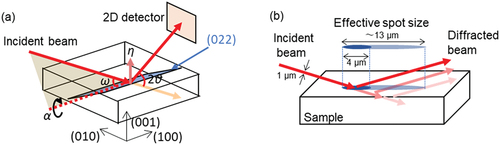
Figure 1 shows schematic illustrations of the optical system of the micro-beam XRD. The measurement was performed at the beamline 11XU of the SPring-8 SR facility. The X-ray wavelength was 1.305 Å and its divergence was negligible. The beam was focused by a Fresnel zone plate to 1 µm in diameter, and its effective spot size, was approximately elliptical with major and minor diameters of 1 and 13 µm considering the incident angle and diffraction from the sample inside, as shown in Figure 1 (b). The spatial mapping was performed on an area of 150 × 150 µm² in 5 µm steps; thus, diffraction measurement was conducted at a total of 31 × 31 = 961 positions. The diffraction patterns from the (022) plane, which was inclined 45° from the sample surface, were detected by a two-dimensional X-ray detector (PILATUS 100K). The pixel number and angular resolution of the detector were 487 × 195 pixels and 0.014078°, respectively. To capture small variations in diffraction conditions corresponding to the spatial distribution of SiGe composition and crystal orientation, the diffraction patterns were integrated in approximately 3° rotational steps around the η axis at each position.

Figure 1. Schematic illustrations of the optical system of micro-beam XRD. (a) The incident X-ray beam was focused on the sample surface and the XRD pattern from the (022) plane was captured by a two-dimensional detector. Before the spatial mapping, the optical axes, α, ω, θ, and η, were adjusted to the (022) diffraction condition. (b) The effective spot size was estimated to be 13 μm in major diameter taking incident angle and diffraction from sample inside into account.

Before the unsupervised machine learning, the measured XRD patterns were pre-processed. The diffraction pattern images were resized from 487 × 195 pixels to 122 × 48 pixels, and the pattern area 33 × 33 pixels covered both the Si and Ge diffraction spots were cut off. In addition, the image intensity was converted to the natural logarithm scale. A diagram of these pre-processings is shown in Figure S1 in the supplemental information. Note that the resize processing has almost no effect on the conclusions of the analysis using NMF. An example of the NMF result for the XRD images without the resize processing is provided in Figure S2 in the supplemental information.

2.2. SiGe sample and XRD patterns

A (001) SiGe film on a (001) Si substrate grown by screen printing and firing [35] was used as a test sample for the spatial mapping of XRD patterns. The thickness and average composition of the film were approximately 20 µm and Si_0.7Ge_0.3, respectively. A sample with large spatial variation in composition on the micrometre scale was selected. Mapping by micro-beam XRD can reveal the spatial distribution of both composition and crystal orientation. These physical properties are important for applications to electrical and optical devices as well as for fundamental investigation of the crystal growth mechanism in aluminium-induced crystallization.

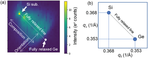
Figure 2 shows the average pattern of 961 XRD patterns around (220) diffraction spots of Si and SiGe obtained in the spatial mapping. The sharp bright spot in the upper left and the broad patterns spread below and to the right are diffraction spots from the Si substrate and SiGe film, respectively. The positions of the Si substrate and the white dot are equivalent to pure Si and Ge, respectively. Thus, the diagonal line from the Si spot to the Ge spot corresponds to fully relaxed SiGe, and the direction along this diagonal corresponds to the SiGe composition. The normal direction to the fully relaxed SiGe line corresponds to the tilt of the crystal orientation of the SiGe film around the X-ray incident direction on the sample surface. It should be noted that the SiGe film was almost fully relaxed because the film was much thicker than the critical thickness of epitaxial Si_0.7Ge_0.3 on a Si substrate. Therefore, the position of the SiGe spots in the orientation direction solely indicates the crystal orientation of the fully relaxed SiGe film without uniaxial lattice deformation. This is also supported by the distribution of SiGe spots that appeared line-symmetrically with the fully relaxed SiGe line and not aligned with the vertical line from the Si substrate spot. The measured SiGe film has spatially local domains with slight inclinations less than 0.5º in crystal orientation. Although all the SiGe domains of the film were almost fully relaxed, in this paper ‘fully relaxed line’ is specifically used for the line connecting the Si substrate spot and the fully relaxed Ge spot, according to the convention.

Figure 2. (a) Average pattern around (220) SiGe diffraction spots of 961 XRD patterns obtained in the spatial mapping. The pixel resolution and intensity were converted to 1/4 and the natural logarithm scale from the original two-dimensional detector image. The white dot shows the position corresponding to the (220) diffraction spot of fully relaxed Ge. (b) Positions of (220) diffraction spots of pure Si and Ge in the reciprocal space.

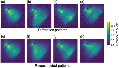
Figure 3 (a–d) show diffraction patterns at different positions on the sample surface. The diffraction patterns have a large variation from one another, reflecting the spatial fluctuation of the composition and crystal orientation of the SiGe film. For example, whereas SiGe spots appear near the Si spot along the fully relaxed line from upper left to lower right in Figure 3 (a), SiGe spots are observed below and above the fully relaxed line in Figure 3 (b–d), respectively. Two SiGe spots appear near the spots of Si substrate and fully relaxed Ge in Figure 3 (c). The number of SiGe spots is not constant, neither are their positions fixed. For the analysis of such complicated patterns, the conventional peak fitting method, based on analyzing the position and intensity of specific peaks, is not able to be conducted automatically and needs manual determination of peak numbers and their initial position by experts. It is almost impossible to perform this process onto the thousands of diffraction patterns. To overcome this issue, we applied NMF to summarize the variation of the diffraction patterns as a few feature patterns and utilized the coefficients of the feature patterns to evaluate the spatial distribution of the composition and crystal orientation.

Figure 3. (a–d) typical XRD patterns obtained in the spatial mapping. The measured positions of (a–d) in the mapping area on the sample surface are (60, 150), (100, 135), (35, 65), (120, 55) in (x, y) in μm. The pixel resolution and intensity were converted to 1/4 and the natural logarithm scale from the original pattern measured by the two-dimensional detector. (e–h) XRD patterns reconstructed for the pattern (a–d) using the four feature patterns and their coefficents obtained through NMF. The reconstructed patterns using the other numbers (1–5) of feature patterns are provided in S5 in the supplemental information.

2.3. Feature extraction via unsupervised machine learning and visualization

XRD data implicitly contain a combination of several ‘basic’ features such as crystal composition and orientation. To automatically extract such features from the observed XRD patterns, we employed NMF [36,37], an unsupervised machine learning method. For given data vectors $x_1,\cdots ,x_n$, NMF aims to approximate each x_i by the linear combination

(1) ${\mathit{x}}_{\mathit{i}}\approx {\sum }_{\mathit{j}=1}^{\mathit{m}}{c}_{\mathit{i},\mathit{j}}{\mathit{s}}_{\mathit{j}}$(1)

where c_i,j ≥ 0, i = 1,$\cdots$, n, j = 1,$\cdots$, m are non-negative combination coefficients and s_j ≥ 0, j = 1,$\cdots$, m, are basis vectors whose elements are non-negative. In matrix notation, the goal of NMF is to find two matrices, C = (c_i,j)_i,j and S = [s₁,$\cdots$, s_m], such that CS ≈ X = [x₁,$\cdots$, x_n]. This is equivalent to approximating the matrix X with a lower-rank matrix. NMF tends to make the coefficient matrices C and S sparse because of the non-negative constraints. This can be viewed as an operation that approximates the data matrix X via a combination of a small number of bases that are uncorrelated with each other. The learning problem to obtain the matrices C and S is formulated as follows [38]:

(2) $\underset{\mathit{C},\mathit{S}}{min}\frac{1}{2}||\mathit{X}-\mathit{CS}||{ }^2+\mathit{\alpha \lambda }\left(||\mathit{vec}\left(\mathit{C}\right)||{ }_1+\mathit{vec}\left(\mathit{S}\right)||{ }_1\right)+\frac{1}{2}\mathit{\alpha }\left(1-\mathit{\lambda }\right)\left(||\mathit{C}||{ }^2+||\mathit{S}||{ }^2\right),$(2)

subject to $c_{\mathit{ij}}\ge 0,{\mathit{s}}_j\ge 0$

where for a matrix A, $\mathit{A}$ and $\mathit{vec}\left(\mathit{A}\right){ }_1={\sum }_{\mathit{i},\mathit{j}}\left|A_{\mathit{i},\mathit{j}}\right|$ represent the Frobenius norm and the element-wise L₁ norm of A, respectively. The first term of (2) is called the reconstruction error and has the effect of approximating X as much as possible with CS. The second term has the effect of inducing sparseness in C and S. The third term is the usual L₂ regularization. α and λ are hyperparameters that control the strength of the regularization (especially the number of bases). In this study, we did not use these regularizations, i.e. α was set to 0 because it is not reasonable to impose equivalent constraints on the spatial distribution and XRD pattern from a physical point of view. The spatial distributions and the XRD patterns have obviously different continuity and sparsity in their two-dimensional patterns. The spatial distribution changes continuously and gradually, while the diffraction pattern is fundamentally a superposition of diffraction spots from the crystalline elements within the incident X-ray spot. Thus, we solved the following equation as the simple application of NMF.

(3) $\underset{\mathit{C},\mathit{S}}{min}\frac{1}{2}||\mathit{X}-\mathit{CS}||{ }^2,$(3)

subject to $c_{\mathit{ij}}\ge 0,{\mathit{s}}_j\ge 0$

Furthermore, instead of the L₁ and L₂ regularization, we applied the following constraint only on the spatial distribution. The learning process of NMF is performed independently on each element of the diffraction patterns and spatial distributions and does not consider the relationship between the spatial positions. This means that there is no matter if the position of two spatial pixels is counterchanged. However, actually, the composition and orientation in the spatial maps are expected to be changed continuously and smoothly on a larger scale than the probe size of the X-ray beam. Such continuousness and smoothness cannot be taken into account by commonly used regularizations such as L₁ and L₂ in Equation (2). We implemented the spatial continuousness on NMF constraining the values of adjacent positions. The spatial constraint on the matrix C was implemented constraining the values of adjacent positions. The following term was added to Equation (3).

(4) $\mathit{\beta }||\mathit{A}||,$(4)

$A_{\mathit{i},\mathit{j}}={\sum }_{\mathit{m},\mathit{n}}{k}_{\mathit{mn}}{C}_{\left(\mathit{i}+\mathit{m},\mathit{j}+\mathit{n}\right)},$

$\mathit{k}=\frac{1}{9}\left(\begin{array}{ccc}-1& -1& -1\\ -1& 8& -1\\ -1& -1& -1\end{array}\right)$

where k is a kernel function to calculate the differential between the adjacent positoins. β is a hyperparameter that controls the strength of the regularization. β = 0 means no constraints and is equivalent to the simple NMF.

In this study, for the simple NMF without the spatial constraint, the 33 × 33 pixel image patterns were each converted to a 1089-dimensional vector, and these vectors were concatenated to construct the data matrix X of size 1089 × 961, where 961 is the sample size. In practice, we used NMF implemented in Python, scikit-learn ver. 0.21 [39]. From 1 to 10 numbers of features were tested. Then, the coefficients of the measured patterns of each feature pattern were calculated.

For the NMF with the spatial constraint, the diffraction pattern images were down pixels to 16 × 16, and the spatial resolution, i.e. the number of the diffraction patterns were reduced to 15 × 15. Thus, the size of the data matrix X was 256 × 225. We implemented the NMF with the spatial constraint in Python as a simple minimization of Equations (3)(3) $\underset{\mathit{C},\mathit{S}}{min}\frac{1}{2}||\mathit{X}-\mathit{CS}||{ }^2,$(3) and (4(4) $\mathit{\beta }||\mathit{A}||,$(4) ) using Limited-memory Broyden – Fletcher – Goldfarb – Shanno algorithm for Bound-constrained optimization (L-BFGS-B) method in the optimization library, Scipy ver. 1.7.1 [40]. The number of the features was fixed to be four and various β values were tested. As in the case of the simple NMF, the coefficients of the measured patterns of each feature pattern were calculated and the spatial distributions were plotted.

For the visualization of spatial mapping of the coefficient matrix C, the coefficients vector for each feature pattern C_j = [c_1j,$\cdots$, c_nj] was transformed to n_x × n_y matrix corresponding to the spatial position of the mesh grid on the sample surface, where n_x and n_y are number of spatial meshes in x and y-direction of the sample stage. Then the spatial distribution of the coefficients was visualized as a heat map.

Two different computers were used in this study: a desktop computer and a laptop computer. The detailed specifications of the computers are summarized in table S3 in the supplemental information.

3. Results and discussion

3.1. Simple NMF

Figure 4 shows feature patterns obtained through NMF on 961 diffraction patterns of the spatial mapping. The number of components, which is a given hyperparameter, was changed from 1 to 10: The results with 1–6 and 1–10 components are shown in Figure 4 and S4 in the supplemental information, respectively. As shown in Figure 4 (g), the position of diffraction spots in the diffraction pattern image represents the composition and crystal orientation of the SiGe film. The position in the direction along the fully relaxed line between the Si substrate and pure Ge represents the SiGe composition. The area below and above the fully relaxed line represent the crystal orientation of left and right tilted around the incident X-ray beam, respectively. From the viewpoint of this crystallographic meaning of the diffraction spots in the reciprocal space, the obtained feature patterns are able to be interpreted. The feature patterns in the first, second, third, and fourth columns correspond to the diffraction pattern of typical SiGe films with high Si composition, left-tilted orientation, low Si composition, and right-tilted orientation. With further increase of the features, the feature patterns are segmentalized to patterns with specific meaning, e.g. in the case of six features in Figure 4 (f), the left-tilted feature patterns in the second column of four features in Figure 4(d) are split into the patterns in the second and sixth columns that correspond to high and low Ge composition.

Figure 4. Feature patterns obtained by NMF with (a) one, (b) two, (c) three, (d) four, (e) five, and (f) six components. The order of the patterns was sorted to be similar patterns are arranged vertically for easy comparison. Dead pixels in the patterns are caused by the dead pixels of the detector. The feature patterns with 1–10 components are provided in S4 in the supplemental information. (g) Corresponding reciprocal space coordinate of the feature pattern images. The position in the direction along the fully relaxed line between the Si substrate and pure Ge represents the SiGe composition. In terms of crystal orientation, the position on the fully relaxed line corresponds to the crystal orientation alined to the Si substrate, and the area below and above the line represents the crystal orientation of left and right tilted around the incident X-ray beam, respectively. (h) Reconstruction error, which is evaluated by the Frobenius norm of the matrix difference in Equation (1) divided by the number of the diffraction patterns, for the 961 diffraction patterns of the models with one to six components. Reconstruction error with 1–10 components is also provided in S4 in the supplemental information.

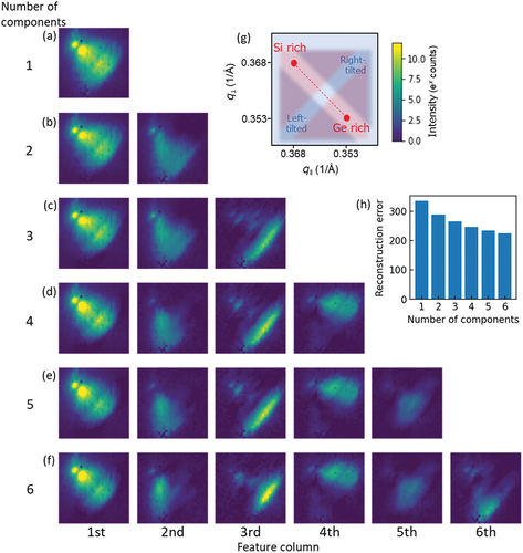
Such a set of feature patterns at the specific feature number interpreted from the viewpoint of XRD pattern meaning is helpful to extract the useful information about the sample, while the reconstruction error consequently decreases with the increase in the number of the features, as shown in Figure 4 (h). Among the feature patterns based on different component numbers, those obtained with four components (Figure 4 (d)) were most useful for the basic analysis of composition and orientation of the SiGe film, because these four patterns are typical patterns that show the SiGe film characteristics as mentioned above. We analyzed the maximum intensity position of the four feature patterns of Figure 4 (d), and calculated the composition and tilt angle of crystal orientation. The results are summarized in Table 1. The four patterns evidently correspond to the diffraction pattern of typical SiGe films with high Si composition, left-tilted orientation, low Si composition, and right-tilted orientation. The reconstructed diffraction patterns for Figure 3 (a–d) using the four feature patterns and their coefficients are shown in Figure 3 (e–h). The reconstructed patterns with one to six components are provided in S5 in the supplemental information. The reconstructed patterns using the four feature patterns surely capture the characteristics of the original diffraction patterns, while the patterns reconstructed using features less than four cannot distinguish the difference of the patterns. This also supports that the four features contain the fundamental characteristics and thus, we used these four feature patterns for the basic analysis of the spatial distribution of the composition and crystal orientation.

Table 1. Composition and tilt angle of crystal orientation calculated from the maximum spot position of the feature patterns of FIG. 4 (d). Positive tilt angle corresponds to left tilt.

Pattern No.	1	2	3	4
Composition	Si1.00Ge0.00	Si0.52Ge0.48	Si0.00Ge1.00	Si0.61Ge0.39
Tilt angle	0º	0.064º	0º	−0.087º

We calculated the coefficients of the measured 961 diffraction patterns for the four feature patterns, and summarized the calculated values as spatial mapping images. Figure 5 (a,b) shows the spatial mapping of the differences of the coefficients, i.e. (coef. 4) – (coef. 2) in (a) and (coef. 3) – (coef. 1) in (b). As discussed above, feature patterns 1 and 3, and 2 and 4 of Figure 4 (c) correspond to high and low composition, and left and right orientation, respectively. Therefore, the differences between their coefficients represent the crystal orientation and Ge composition, respectively. Higher and lower values of Figure 4 (a) correspond to right-tilted and left-tilted and those of Figure 4 (b) correspond to Ge rich and Si rich, respectively.

Figure 5. Spatial mapping images of the coefficients: (a) (coef. 4) – (coef. 2) and (b) (coef. 3) – (coef. 1) of the four feature pattens, and (c) coef. 6 of the six feature pattens. The orientation of both images along the direction from bottom left to top right is caused by the shape of the footprint of the X-ray beam.

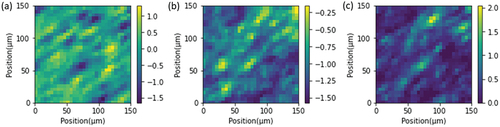
From the viewpoint of characterization of SiGe film, important information could be obtained from the spatial distributions of crystal orientation and composition quantified as Figure 5 (a,b), although the obtained values are relative. We can evaluate the spatial scale of the fluctuations that is several tens of µm and almost equal to spatial fluctuation of SiGe composition obtained using scanning electron microscope with energy-dispersive X-ray spectroscopy. It was also found by statistical analysis that crystal orientation and composition independently fluctuate. They have almost no correlation with each other: Pearson correlation coefficient (Pcc) was −0.14 and the scatter plot of them is provided in S6 in the supplemental information. Pcc shows near 1 and 0 when the two sets of data have a strong positive linear correlation and no correlation, respectively. We are also able to determine the characteristic positions such as high Ge composition or largely tilted crystal orientation. Long-term measurements, such as a scan around the η axis, at such characteristic positions will give a detailed structure of the film. These information about spatial scale, distribution correlation, and characteristic position helps study the formation mechanism of the SiGe film.

Furthermore, utilizing the higher order of feature patterns that have more specific physical meaning, we can identify the position with more specific characteristic, while the four feature patterns can extract the most general characteristics of crystal orientation and composition. One example is shown in Figure 5 (c). The spatial distribution of the coefficient of the sixth column pattern in Figure 4 (f) was calculated. The feature pattern has a broad spot in left tilted orientation and high Ge composition area; consequently, the spatial positions having such characteristics were selectively visualized. In Figure 5 (b), there are several island spots with high Ge composition. Among them, the islands with left-tilted orientation were distinguished by using the feature pattern with a more specific meaning. As demonstrated here, giving the feature patterns physical meaning and analyzing the spatial distribution of their coefficients is useful for the estimation of spatial fluctuation scale and the identification of the characteristic positions.

One of the advantages of this method is that spatial distribution of feature coefficients related to physical properties can be obtained at high speed with low calculation cost. The typical computational time for the training of the 961 XRD patterns was less than 1 minute using the laptop computer. Furthermore, by pretraining the feature patterns using similar sample data, we can calculate the coefficients within 1 second for the case of 961 XRD patterns. This is important in synchrotron radiation experiments where the experimental period is limited. Conventional peak fittings for each diffraction pattern are time-consuming, and it is difficult to analyze a number of patterns and to obtain a spatial map within the experimental period. On the other hand, NMF can provide a spatial map immediately after the measurement on-site. The spatial information is useful to evaluate the spatial size of the fluctuation and to find characteristic position, even though the value is a relative value. For example, it is possible to perform another measurement such as a long-time scan in three-dimensional reciprocal space at the specific position where the feature coefficient intensity is high based on the spatial map, in the same experimental time.

Another advantage is the acquisition of unexpected features patterns. The feature patterns obtained by NMF are an effective means to summarize the variation of the diffraction patterns. Thus, the feature patterns surely contain information of the variety of the diffraction patterns of which a part we may miss. The four feature patterns obtained in this study are consistent with our prior crystallographic knowledge implies that composition and crystal orientation vary in the crystalline film. This simple situation is due to the growth condition under which the SiGe film becomes fully relaxed. In contrast, the sixth feature pattern in Figure 4 (f) provides the information that there are high Ge and left-tilted regions in the sample. The spatial distribution of such a characteristic region is visualized by mapping its coefficient as shown in Figure 5 (c). In the case of strained film, fluctuation would become more complicated; consequently, an unexpected set of feature patterns, such as line-like patterns tailed in one direction, may be obtained. Such unexpected data-driven feature patterns will be useful for the analysis in a new light, which may result in new findings.

It should be noted that the background pattern is also decomposed into the feature patterns through NMF. For example, the diffraction spot of Si commonly appears in the diffraction patterns as shown in Figure 3, and thus, it is a background pattern. However, the Si substrate spot mainly decomposed into the Si-rich SiGe feature pattern as shown in Figure 4, although it should be separated from the SiGe features. Modeling of the background, such as proposed in Ref.36, will solve this problem.

3.2. NMF with spatial constraints

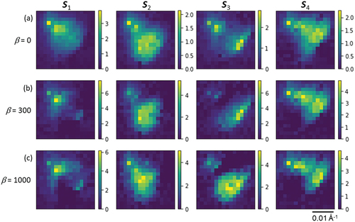
Figure 6 shows the feature patterns obtained through NMF using spatial constraints of β = 0, 300, 1000. Comparing the feature patterns of β = 0 (Figure 6 (a)) to those in Figure 4 (d), it is found that almost the same feature patterns were obtained also in the case of the reduced pixel resolution and fewer data sizes. These patterns correspond to the diffraction pattern of typical SiGe films with high Si composition, left-tilted orientation, low Si composition, and right-tilted orientation.

Figure 6. Feature patterns S_j obtained throuth NMF with spatial contraints, β = 0, 300, 1000 for (a), (b), (c). The virtical and horizontal direction correspond to q_⊥ and q_‖ in the reciprocal space, as in the case of FIG. 4. The order of the patterns was sorted to be similar patterns are arranged vertically for easy comparison. The subscript number j of S corresponds to the feature number common to those in FIG.7. The feature patterns obtained with other β values are provided in S7 in the supplemental information.

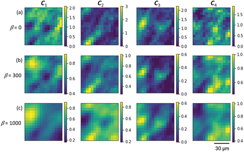
Figure 7 shows the spatial distribution of coefficients of the feature patterns obtained through NMF using spatial constraints of β = 0, 300, 1000. The four distributions correspond to the coefficients of the patterns in Figure 6 with the same subscription. It is found that the values of the coefficients are surely non-negative, and the spatial distribution becomes smooth with increasing the strength of the spatial constraint, β. The spatial distribution of β = 0, i.e. without the spatial constraint, is seen to have a random spot-like noise. Most spots are expected to be artifacts due to NMF because the SiGe film used in this study rarely has such a strong fluctuation in local areas smaller than the mapping step size, 5 μm. This noise was suppressed by the spatial constraint, and the spatial distribution with β = 300 shows the reasonable smoothness and continuousness of the composition and crystal orientation in terms of the domain structure of the SiGe film. Further increase of the spatial constraint leads to the blurriness of the domain shapes as shown in Figure 7 (c). These results demonstrate that the introduction of spatial constraint gives a more reasonable spatial distribution which provides a more precise evaluation of the shape of the spatial fluctuation and identification of the characteristic position.

Figure 7. Spatial distribution of the coefficients C_j of the four features with spatial contraints, β = 0, 300, 1000. The subscript number j of C corresponds to the feature number in FIG.6. The spatial size of the images is 75 μm × 75 μm. The feature patterns obtained with other β values are provided in S8 in the supplemental information.

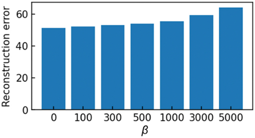
Here, it is a difficult problem to determine the appropriate strength of the spatial constraint, β value. We evaluated the reconstruction error of the models learned with different β, and the result is shown in Figure 8. The reconstruction error increases with increasing in β. This trend is similar to the other regularizers, such as L1 and L2 norms. However, minimum reconstruction error is not the most reasonable criterion to determine β as discussed above. It might be the best way to determine heuristically considering the balance between the reconstruction error and spatial smoothness on the basis of physical knowledge. In the future, it will be possible that information on the spatial fluctuation-scale size to be used to control the constraint through the constraint kernel function when the scale is given by other methods.

Figure 8. Reconstruction error of the models learned with different β. The error was evaluated by Frobenius norm of the matrix difference in Equation (2) divided by the number of the diffraction patterns.

It should be commented on the computational cost for the NMF with the spatial constraints. The typical computational time for the training of the 225 resized XRD patterns for the NMF with spatial constraints was approximately 10 hours using the desktop computer. This high computational cost is due to simple implementation without techniques to reduce the cost, and it can be significantly reduced by adapting efficient calculation techniques, such as Coordinate descent [35], Multiplicative Update [36], and MiniBatchNMF [41], but it is out of the scope of this paper.

4. Conclusions

In summary, we applied NMF to the analysis of a number of XRD patterns from a crystalline SiGe film with spatial fluctuation in both composition and orientation. The obtained feature patterns, with various numbers of features, show typical diffraction patterns from SiGe films with high and low composition and right- and left-tilted orientation. The spatial mapping of the differences between the coefficients of the diffraction patterns at each position on the feature patterns illustrated the distributions of composition and crystal orientation. Furthermore, by selecting an appropriate feature pattern with specific physical meaning, such as high Ge composition and left-tilted crystal orientation, the characteristic regions were extracted from the mapping area through a similar scheme with the coefficient calculation of the feature patterns. The computational cost of these analyses is significantly smaller than the conventional peak fitting analysis, and consequently, it can be conducted within an SR experimental period. Thus, we can perform another measurement at the characteristic position found by the NMF analysis. In addition, the introduction of spatial constraint to NMF gives more reasonable spatial distributions to realize the continuousness and smoothness of the SiGe domain structure. These analyses will give a wider experimental opportunity in XRD measurements.

Author contributions

K.K. designed this project and performed the machine learning. S.T., S.F. and M.T. conducted the XRD measurements. I.T. and K.M. contributed to the theoretical discussion. K.K., T.K., T.S., S.T., S.F. and M.T. discussed the results of machine learning modeling. K.K. and K.M. wrote the paper. All the authors discussed the results and commented on the paper.

Acknowledgements

The authors acknowledge Mr. Fukami, Prof. Usami and Prof. Ujihara of Nagoya University and Mr. Nakahara and Dr. Marwan of Toyo Aluminium K.K. for their sample provision and fruitful discussions.

Disclosure statement

No potential conflict of interest was reported by the author(s).

Data availability statement

The data and the code that support the findings of this study can be found at https://github.com/KentaroKutsukake/NMF-for-XRD.git.

Supplementary material

Supplemental data for this article can be accessed online at https://doi.org/10.1080/27660400.2024.2336402.

Additional information

Funding

The synchrotron radiation experiments were performed at the 11XU of SPring-8 with the approval of the Japan Synchrotron Radiation Research Institute (JASRI) (Proposal No. 2016A3553, 2017A3553, 2017B3553, 2018A3553, 2018A3585, 2018B3553, 2018B3587, 2019A3587, 2019B3586, and 2020A3586). This study was supported by QST microstructural characterization platform as a program of “Nanotechnology Platform” of the Ministry of Education, Culture, Sports, Science and Technology (MEXT), Japan, and Center for Advanced Intelligence Project, RIKEN.

References

- Miao J, Charalambous P, Kirz J, et al. D. Extending the methodology of X-ray crystallography to allow imaging of micrometre-sized non-crystalline specimens. Nature. 1999;400(6742):342. doi: 10.1038/22498
- Robinson I, Harder R. Coherent X-ray diffraction imaging of strain at the nanoscale. Nat Mater. 2009;8(4):291. doi: 10.1038/nmat2400
- Tamura N, Celestre RS, MacDowell AA, et al. Submicron x-ray diffraction and its applications to problems in materials and environmental science. Rev Sci Instrum. 2002;73(3):1369. doi: 10.1063/1.1436539
- Nikitenko S, Beale AM, Eerden MJ, et al. Implementation of a combined SAXS/WAXS/QEXAFS set-up for time-resolved in situ experiments. J Synchrotron Rad. 2008;15(6):632. doi: 10.1107/S0909049508023327
- Mimura H, Handa S, Kimura T, et al. Breaking the 10 nm barrier in hard-X-ray focusing. Nat Phys. 2010;6(2):122. doi: 10.1038/nphys1457
- Chao W, Fischer P, Tyliszczak T, et al. Real space soft x-ray imaging at 10 nm spatial resolution. Opt Express. 2012;20(9):9777. doi: 10.1364/OE.20.009777
- Mohacsi I, Vartiainen I, Rösner B, et al. Interlaced zone plate optics for hard X-ray imaging in the 10 nm range. Sci Rep. 2017;7(1):43624. doi: 10.1038/srep43624
- Denes P, Doering D, Padmore HA, et al. A fast, direct x-ray detection charge-coupled device. Rev Sci Instrum. 2009;80:083302. doi: 10.1063/1.3187222
- Denes P, Schmitt B. Pixel detectors for diffraction-limited storage rings. J Synchrotron Rad. 2014;21(5):1006. doi: 10.1107/S1600577514017135
- Kameshima T, Ono S, Kudo T, et al. Development of an X-ray pixel detector with multi-port charge-coupled device for X-ray free-electron laser experiments. Rev Sci Instrum. 2014;85(3):03110. doi: 10.1063/1.4867668
- Sasaki T, Suzuki H, Sai A, et al. In situ Real-Time X-ray reciprocal space mapping during InGaAs/GaAs growth for understanding strain relaxation mechanisms. Appl Phys Express. 2009;2:08550. doi: 10.1143/APEX.2.085501
- Richard MI, Highland MJ, Fister TT, et al. In situ synchrotron x-ray studies of strain and composition evolution during metal-organic chemical vapor deposition of InGaN. Appl Phys Lett. 2010;96(5):051911. doi: 10.1063/1.3293441
- Hu W, Suzuki H, Sasaki T, et al. High-speed three-dimensional reciprocal-space mapping during molecular beam epitaxy growth of InGaAs. J Appl Crystallogr. 2012;45(5):1046. doi: 10.1107/S0021889812036175
- Jung J, Yoon J, Park HK, et al. Microstructure design using machine learning generated low dimensional and continuous design space. Materialia. 2020;11:100690. doi: 10.1016/j.mtla.2020.100690
- Ramirez JM, Liu Q, Vakarin V, et al. Graded SiGe waveguides with broadband low-loss propagation in the mid infrared. Opt Express. 2018;26(2):870–12. doi: 10.1364/OE.26.000870
- Kutsukake K, Usami N, Ujihara T, et al. On the origin of strain fluctuation in strained-si grown on SiGe-on-insulator and SiGe virtual substrates. Appl Phys Lett. 2004;85(8):1335–1337. doi: 10.1063/1.1784036
- Nagata K, Sugita S, Okada M. Bayesian spectral deconvolution with the exchange Monte Carlo method. Neural Networks. 2012;28:82–89. doi: 10.1016/j.neunet.2011.12.001
- Matsumura T, Nagamura N, Akaho S, et al. Spectrum adapted the expectation-maximization algorithm for high-throughput peak shift analysis. Sci Technol Adv Mater. 2019;20(1):733–745.
- Shinotsuka H, Nagata K, Yoshikawa H, et al. Development of spectral decomposition based on Bayesian information criterion with estimation of confidence interval. Sci Technol Adv Mater. 2020;21(1):402–419. doi: 10.1080/14686996.2020.1773210
- Lee DD, Seung HS. Learning the parts of objects by non-negative matrix factorization. Nature. 1999;401(6755):788–791. doi: 10.1038/44565
- Lee D, Seung HS. Algorithms for non-negative matrix factorization. Adv Neural Inf Process Syst. 2001; 13.
- Friedman J, Hastie T, Tibshirani R. The elements of statistical learning. In: Bühlmann P, Diggle P, Gather U, editors. Volume 1 Springer series in statistics. New York (NY): Springer; 2001.
- Cichocki A, Zdunek R, Phan A, et al. Nonnegative matrix and tensor factorizations: applications to Exploratory Multi-way Data Analysis and blind source separation. New Jersey: Wiley; 2009.
- Févotte C, Bertin N, Durrieu JL. Nonnegative matrix factorization with the Itakura-Saito divergence: with application to music analysis. Neural Comput. 2009;21(3):793–830. doi: 10.1162/neco.2008.04-08-771
- Honma M, Akiyama K, Uemura M, et al. Super-resolution imaging with radio interferometry using sparse modelling. Publ Astron Soc Jpn. 2014;66(95):1–14.
- Shiga M, Tatsumi K, Muto S, et al. Sparse modeling of EELS and EDX spectral imaging data by nonnegative matrix factorization. Ultramicroscopy. 2016;170:43–59. doi: 10.1016/j.ultramic.2016.08.006
- Long CJ, Bunker D, Li X, et al. Rapid identification of structural phases in combinatorial thin-film libraries using x-ray diffraction and non-negative matrix factorization. Rev Sci Instum. 2009;80(10):103902.
- Kusne AG, Keller D, Anderson A, et al. High-throughput determination of structural phase diagram and constituent phases using GRENDEL. Nanotech. 2015;26(44):444002. doi: 10.1088/0957-4484/26/44/444002
- Stefano S, Bras RL, Suram SK, et al. Pattern decomposition with complex combinatorial constraints: application to materials discovery. Proc Twenty-Ninth AAAI Conf Art Int. 2015;29(1). doi: 10.1609/aaai.v29i1.9233
- Bai J, Bjorck J, Xue Y, et al. Relaxation methods for constrained matrix factorization problems: solving the phase mapping problem in materials discovery. International Conference on AI and OR Techniques in Constraint Programming for Combinatorial Optimization Problems. Springer, Cham; 2017. doi: 10.1007/978-3-319-59776-8_9
- Suram SK, Xue Y, Bai J, et al. Automated phase mapping with AgileFD and its application to light absorber discovery in the V–mn–nb oxide system. ACS Comb Sci. 2016;19(1):37–46.
- Stanev V, Vesselinov VV, Kusne AG, et al. Unsupervised phase mapping of X-ray diffraction data by nonnegative matrix factorization integrated with custom clustering. Npj Comput Mater. 2018;4:43. doi: 10.1038/s41524-018-0099-2
- Jha D, Kusne AG, Bahrani RA, et al. Peak area detection network for directly learning phase regions from raw x-ray diffraction patterns. 2019 International Joint Conference on Neural Networks (IJCNN). IEEE; 2019: pp.1–8. doi: 10.1109/IJCNN.2019.8852096
- Fukami S, Nakagawa Y, Hainey MF Jr, et al. Epitaxial growth of SiGe on Si substrate by printing and firing of Al–ge mixed paste. Jpn J Appl Phys. 2019;58(4):045504–1–6. doi: 10.7567/1347-4065/ab00e5
- Cichocki A, PHAN A-H. Fast local algorithms for large scale nonnegative matrix and tensor factorizations. IEICE Trans Fundamentals. 2009;92(3):708–721. doi: 10.1587/transfun.E92.A.708
- Fevotte C, Idier J. Algorithms for nonnegative matrix factorization with the beta-divergence. Neural Comput. 2011;23(9):2421–2456. doi: 10.1162/NECO_a_00168
- Hoyer P. Non-negative matrix factorization with sparseness constraints. J Mac Learn Res. 2004;5:1457–1469.
- Pedregosa F, Varoquaux G, Gramfort A, et al. Scikit-learn: machine learning in Python. J Mach Learn Res. 2011;12:2825–2830.
- Virtanen P, Gommers R, Oliphant TE, et al. Fundamental algorithms for scientific computing in Python. Nat Methods. 2020;17(3):261–272.
- Ament SE, Stein HS, Guevarra D, et al. Multi-component background learning automates signal detection for spectroscopic data. Npj Comput Mater. 2019;5(1):77. doi: 10.1038/s41524-019-0213-0
- Augustin L, Bach F, Févotte C Online algorithms for nonnegative matrix actorization with the Itakura-Saito divergence. 2011 IEEE Workshop on Applications of Signal Processing to Audio and Acoustics (WASPAA). New Paltz, NY, USA: IEEE; 2011. p. 313–316. doi:10.1109/ASPAA.2011.6082314