An interpretable predictive model for bank customers’ income using the eXtreme Gradient Boosting algorithm and the SHAP method: a case study of an Anonymous Chilean Bank

Abstract

In the dynamic landscape of banking institutions, acquiring accurate and timely information regarding customers’ incomes is crucial for effectively managing financial product offerings. To meet this demand, these institutions construct predictive models using numerous features, with only a subset contributing to capturing income variability. In this study, we propose a methodology for predicting monthly incomes by employing an XGBoost model with a reduced number of features. Feature reduction is accomplished through the implementation of Boruta and BorutaSHAP, ensuring that no predictive power is lost throughout the process. To enhance the transparency of the model’s predictions, we used the Shapley Additive Explanations (SHAP) method. The dataset used was provided by an anonymous bank from Chile, consisting of 10,000 records, 426 features, and a substantial proportion of missing values. The results demonstrate that the combination of feature selection methods and the XGBoost algorithm enables the development of a more concise model that maintains predictive performance. By leveraging the SHAP method, financial institutions can consistently identify and track influential features, thereby reducing complexity and training time without compromising predictive power. This research offers valuable contributions to financial institutions, as they can adopt our methodology to consistently identify and track the most influential features.

KEYWORDS:

• Income prediction
• XGBoost
• variable selection
• Boruta
• SHAP

1 Introduction

Income is a demographic factor related to the economic level, living conditions, satisfaction with the standard of living, and financial well-being of individuals. Additionally, it is a factor closely associated with the consumption level of consumers (Ambrey and Fleming 2014; Burlacu 2016; Bussolo et al. 2018; Yu et al. 2020b). For financial institutions, accurate income prediction is crucial for effectively managing the banking products offered to customers. Generally, these institutions require up-to-date information on their customers’ total income, which encompasses all sources of income (such as wages, salaries, benefits, interest payments, rents, etc.) over a given period, typically one month. Therefore, having models that provide accurate income estimates is of utmost importance. Also, in an era marked by periodic financial crises, the accuracy of income estimates becomes increasingly crucial for informed decision-making (Fuders 2023).

The literature contains several papers on modeling and predicting income or income levels. For instance, Lazar (2004) evaluates income prediction data based on the Current Population Survey provided by the U.S. Census Bureau. Swan (2006) demonstrate that observed characteristics, including gender, age, occupation, industry, and length of paid employment, explain only a small portion of income variability. García-Alonso et al. (2010) elaborate on income predictions in the agricultural sector using models based on neural networks and heuristic methods. Matkowski (2021) show that new models outperform traditional forecasting approaches in predicting individual income. Singh et al. (2021) estimate population income using linear models and data visualization techniques. Other studies have focused on methodologies for estimating the future earnings of college students (e.g., Smart 1988; Thomas 2000; Chia and Miller 2008). However, the prediction of bank customers’ income remains largely unexplored, except for a few exceptions (Kibekbaev and Duman 2016), which can be attributed to the challenge of obtaining accurate information on individuals’ income, wealth, and characteristics.

In recent years, financial institutions have embraced new modeling methodologies that leverage Machine Learning (ML) algorithms and have promoted the adoption of data science-based analysis techniques.¹ According to Molnar (2020), ML is the study of algorithms capable of improving or learning automatically through experience and data. The primary goal of ML algorithms is to relax some of the stringent assumptions in traditional models and enhance prediction accuracy (Vythoulkas and Koutsopoulos 2003). Moreover, ML methods capture complex relationships between variables through data-driven learning (Molnar 2020). ML techniques have been recognized for their computational efficiency and their ability to achieve prediction results superior to those obtained with commonly used statistical methods (e.g., Shin et al. 2021; Lang et al. 2022). However, the main drawback of ML algorithms is their black-box nature (Salas et al. 2022), which has been a key limitation hindering their widespread adoption by the scientific community. In general, using complex ML algorithms brings gains in predictive performance but sacrifices interpretability (Molnar 2020). In the financial context, Futagami et al. (2021) employ ML algorithms to predict future pairings of acquiring and acquired companies for generating acquisition or investment strategies. Ross et al. (2021) develop a machine-learning model called CapitalVX (Capital Venture eXchange) to predict outcomes for startups. Jaquart et al. (2021) use ML algorithms to analyze the predictability of the Bitcoin market over various prediction horizons. Pinelis and Ruppert (2022) find economically and statistically significant benefits of using machine learning for portfolio allocation between the market index and the risk-free asset. Goldberg and Mouti (2022) utilize supervised learning to identify factors that predict the cross-section of returns and maximum drawdown of stocks in the U.S. equity market.

On the one hand, when training a predictive model, the specific reasons behind a decision may not always be relevant. What matters is that the model performs well on a test dataset (Molnar 2020). However, in certain cases, understanding the “why” can provide valuable insights into the problem, the data, and potential model failures. Therefore, it becomes essential to incorporate interpretability or explanation analysis of predictions to build confidence in the trained model. Miller (2017) indicates that interpretability refers to the extent to which a person can comprehend the causes behind a decision. Similarly, Gunning et al. (2019) defines model interpretability as the degree to which inputs explain outputs. The higher the interpretability of an ML model, the easier it becomes to understand the reasoning behind specific decisions or outcomes (Molnar 2020). These measures or significance values can be computed for individual predictions (individualized) or the entire dataset to explain the overall behavior of a model (global) (Lundberg et al. 2018). In this study, we employ the Shapley Additive eXPlanation (SHAP) method, developed by Lundberg and Lee (2017), for interpretability. This method is based on concepts from cooperative game theory. The SHAP method has been widely used to explain ML models across various fields, including soil science (Padarian et al. 2020; Yu et al. 2020a; Silva et al. 2022a), finances (Mokhtari et al. 2019; Futagami et al. 2021; Lin and Gao 2022), transportation (Alsaleh and Farooq 2021; Cai et al. 2022; Fafoutellis et al. 2022), among others. It has consistently demonstrated a stronger alignment with human explanations. Also, the SHAP method is a technique used in machine learning to explain the output of a model by attributing the contribution of each feature to the final prediction. It helps in understanding how the model arrived at a specific decision by quantifying the impact of individual features on the prediction. SHAP values provide a way to interpret complex machine learning models and assess the influence of each feature in the decision-making process (Molnar 2020).

The datasets used for incomes prediction often contain hundreds of explanatory variables or inputs. However, only a small subset of these variables significantly contributes to the model’s performance. Hence, it is crucial to employ techniques that reduce the dimensionality of these datasets. This reduction is essential for improving computation times, preventing overfitting, enhancing predictive accuracy, and facilitating interpreting predictions from more concise models. The challenge of dimensionality is well-recognized in the application of statistical learning algorithms. Authors such as Ładyżyński et al. (2019), Hughes (1968), and Trunk (1979) point out that increasing the number of explanatory variables does not necessarily lead to improved accuracy for specific problems and suggest the existence of an optimal point in terms of the number of explanatory variables, beyond which accuracy starts to decline.

This study employed the Boruta method (Kursa and Rudnicki 2010) and the BorutaSHap method (Keany 2020) for feature selection. These techniques assist us in identifying the most important variables or features for predicting incomes. An anonymous Chilean financial institution provided the dataset used and contains records with NaN values, which represent non-numeric values and missing or incomplete information. Since many predictive modeling algorithms need datasets without NaN values, analysts employ imputation methods or directly remove NaN observations to address this issue. Our approach allows us to incorporate the entire dataset without eliminating NaN values, representing a significant advantage in our work.

This article provides an in-depth analysis of the theoretical and empirical foundations, as well as practical applications, of predicting customer incomes in banking institutions. By leveraging financial data, we present results and findings from a data science perspective, incorporating various tools that enable income prediction with fewer explanatory variables without compromising predictive power. Our study primarily focuses on applying diverse machine-learning techniques to reduce the number of explanatory variables and generate reliable predictions for financial decision-making. Additionally, we demonstrate how these data science advancements contribute to addressing real-world problems and fostering the creation of new financial products. Our work demonstrates an innovative application of data science in financial economics, emphasizing its relevance in the financial services industry and traditional financial research and tackling current challenges.

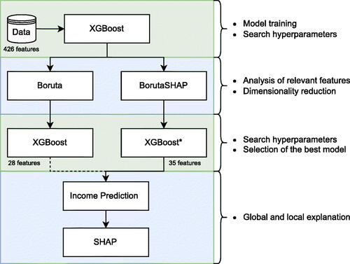
In our study, we utilize the eXtreme Gradient Boosting (XGBoost) algorithm for income modeling and prediction. To reduce the dimensionality of the explanatory variables space and achieve more concise models, we employ the Boruta and BorutaSHAP algorithms and compare their results. Additionally, we leverage recent advances in machine learning to elucidate the predictions of the best XGBoost model through the SHAP method. Figure 1 illustrates the step-by-step process followed in this work.

Fig. 1 Schematic methodology process representation.

The rest of this article is structured as follows. Section 2 describes this study’s principal methods and performance metrics. Then, Section 3 shows the dataset description and main results obtained. Finally, Section 4 closes the paper with concluding remarks, identifying the limitations of the article and suggesting future research directions.

2 Methods

2.1 Extreme gradient boosting (XGBoost)

Boosting is a powerful learning method based on the idea that the sequential process of applying a learning algorithm slightly better than stochastic guessing (weak learner), on modified versions of the data, will generate a strong “committee” (Salas et al. 2022). The Gradient boosting algorithm uses sequential learning, where each weak learner learns from the errors of previous learners; thereby, boosting the entire ensemble. Each learner is trained on sequential modifications of the data, by reweighting each observation according to the misclassified samples from the previous learner. Hence, the misclassified observations become more important for the current learner, thus, its relative weight will be increased. Conversely, the weights of well-classified samples decrease gradually.

Finally, the prediction work by weighted majority voting, which is a well-known optimal decision rule for collective decision making, given the probability of sources to provide accurate information (trustworthiness). According to Wang et al. (2018), the Extreme Gradient Boosting (XGBoost) (Chen and Guestrin 2016) algorithm is a meta-algorithm that allows you to build a model with strong learning power from weaker learners, typically decision trees. Moreover, the XGBoost was designed to optimize resources by using distributed computing(Fan et al. 2018).

2.2 Hyperparameter tunning

Hyperparameter tuning is an essential step in any ML project, so, before the training phase, we must find a set of hyperparameter values that give the best performance of each model on the data in a reasonable time. This process is called hyperparameter optimization or tuning and plays a vital role in the predictive accuracy of the machine learning algorithms (Wu et al. 2019). We use Bayesian Optimization to obtain the optimal parameter settings for XGBoost algorithm. According to Wu et al. (2019) Bayesian optimization combined a prior distribution of a function with sample information (evidence) to obtain posterior of the function; then the posterior information was used to find where the function was maximized according to a criterion.

The hyperparameters selection is done by Python’s hyperopt library (Bergstra et al. 2013). To ensure reproducibility of the results a random seed is set.

2.3 Shapley additive explanations (SHAP)

SHAP by Lundberg and Lee (2017) is a method to explain individual predictions of ML models. SHAP is a game theoretic model explanation method based on Shapley Values (Shapley 1953). Thus, the theoretical SHAP value of the ith covariate for nth individual is calculated as (1) $${\varphi }_i^{(n)}=\sum _{s\subseteq p\left\{i\right\}}\frac{s!(p-s-1)!}{p!}\left[f_{s\cup \left\{i\right\}}(x_{s\cup \left\{i\right\}})-f_s(x_s)\right],$$(1) where p is the total number of covariates, s is a subset of covariates, $f_{s\cup \left\{i\right\}}(x_{s\cup \left\{i\right\}})$ and $f_s(x_s)$ is the prediction from fit model with and without covariate i for individual n, respectively.

The SHAP method is based on the concept that, in order to explain a complex model f it is necessary to use an explanation model g, simpler than the original one (Padarian et al. 2020). This simplification consists in the use of simplified entries $x\prime$ that are mapped to the original entries x through the mapping function $x=h_x(x\prime )$, which is specific to x. Given a different set the input $z\prime \approx x\prime$, the method ensures that $g(z\prime )\approx f(h_x(z\prime ))$. In order to estimate the effect of varying the input x, $z\prime$ is obtained from reference values sampled from other observations from the training dataset. Then, the effect ${\varphi }_i$ to each covariate becomes part of a linear function of binary variables. SHAP specifies the explanation for prediction of observation x as: (2) $$g(x\prime )={\varphi }_0+\sum _{j=1}^M{\varphi }_{j}z{\prime }_j,$$(2) where g is the explanation model, $z\prime \in {\{0,1\}}^M$ is the coalition vector, M is the maximum coalition size and ${\varphi }_j\in \mathbb{R}$ is the covariate attribution for a covariate j, the Shapley values.

SHAP values were calculated for the RF classifier models. SHAP values reflect the magnitude of a explanatory variable’s influence on model predictions. The computation of the SHAP values from training is done by Python’s shap library (Bergstra et al. 2013) using the TreeShap algorithm.

2.4 Explanatory variable selection methods

We used the Boruta (Kursa and Rudnicki 2010) and BorutaShap (Keany 2020) explanatory variable selection methods to select the most important features or explanatory variables to estimate the income. This process is fundamental to improve the performance and the explicability of the regression XGBoost model.

The Boruta algorithm (Kursa and Rudnicki 2010) is based on a Random Forest model (Breiman 2001). Based on the inferences of this Random Forest, explanatory variables are removed from the training set, and model training is performed anew. Boruta infers the importance of each independent variable (explanatory variable) in the obtained predictive outcomes by creating shadow explanatory variables. This helps in the identification of all attributes which are in some circumstances relevant for classification, the so-called all-relevant problem. Finding all relevant explanatory variables, instead of only the non-redundant ones, may be very useful when one is interested in understanding mechanisms related to the subject of interest, instead of merely building a black-box predictive model. Like Alsahaf et al. (2022), we use XGBoost as the base ranking algorithm for Boruta by modifying the code of the BorutaPy Python’s library.

BorutaShap (Keany 2020) is an implementation of the Boruta algorithm. However, the BorutaShap measures the relevance with the SHapley Additive exPlanations (SHAP) metric (Lundberg and Lee 2017) descritos en la Sección Section 2.3. According to Silva et al. (2022b), the use of the SHAP metric improves the original Boruta in quality of the produced variables subset.

2.5 Evaluation metrics

To evaluate predictive performances among different models, we used metrics such as the root mean squared error (RMSE), the mean absolute error (MAE) and hit rates metrics, which give a interval in which the variation between the prediction and the actual value may fall. These metrics are calculated from the following equations. (3) $$\mathit{\text{RMSE}}=\sqrt{\frac{1}{n}\sum _{i=1}^n{(y_i-{\widehat{y}}_i)}^2},$$(3) (4) $$\mathit{\text{MAE}}=\frac{1}{n}\sum _{i=1}^n|y_i-{\widehat{y}}_i|,$$(4) (5) $$H{R}_{\alpha \%}=\frac{1}{n}\sum _{i=1}^{n}I\left\{{\widehat{y}}_i\in [(1-\alpha )y_i,(1+\alpha )y_i]\right\},$$(5) where y_i is the observed income, ${\widehat{y}}_i$ the predicted income, α define the hit rates width, and $I\{·\}$ is an indicator function that takes the value one when the condition is satisfied and zero otherwise.

3 Application

This section presents the results of this study. To enhance our work’s credibility, we analyzed one real-world dataset from an anonymous Chilean bank. The results presented and discussed in this section derive from implementing the previously described methods, viewpoints, and metrics through the Python programming language and its appropriate libraries.

In this work, we used cross-validation method considering a split of original dataset in 70% for training, and the remaining 30% for testing the models. The process of validation and training of XGBoost models is performed using Python’s Scikit-Learn library (Pedregosa et al. 2011). The hyperparameters tunning for each model is done by Python’s hyperopt library (Bergstra et al. 2013). To ensure reproducibility of the results a random seed is set.

3.1 Data

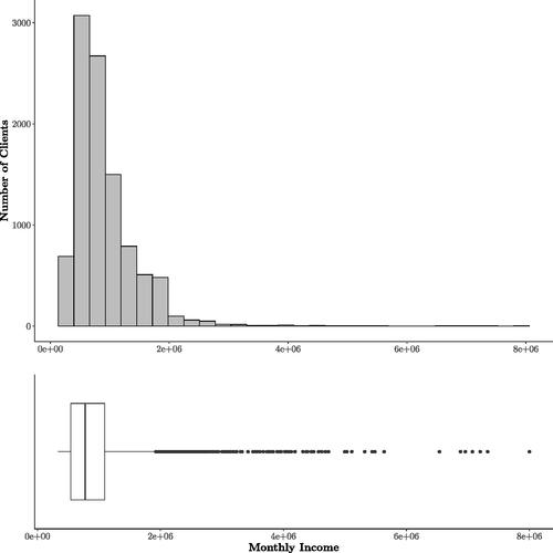
The dataset contains 10.000 observations (client records) and 426 explanatory features or Variables. The response variable income corresponding to the average monetary income of three consecutive months. For confidentiality reasons, we changed the name of the explanatory variables to $x_1,x_2,\dots ,x_{426}$, replacing their original names. The descriptive analysis of the response variable shows an asymmetric behavior. Specifically, it can be seen in Figure 2 that there is a higher concentration of clients with an average income of less than one million of Chilean peso (CLP). In addition, there are very extreme values to the right of the distribution. Also, there is 31.7% of the data corresponds to a NaN value. These missing values are relevant to the financial institution and will not be discarded from the analysis or the XGBoost training. The results from the methodology proposed in this work are presented below (see Figure 1).

Fig. 2 Observed monthly income distribution.

3.2 Models specification

The initial model is trained using the records of the 426 explanatory variables, taking the default values for the algorithm’s hyperparameters; this model is referred to as M1. Subsequently, recognizing the importance of hyperparameters in the training process of ML algorithms, we conducted a search for these using the Bayesian framework mentioned earlier. Through this process, we obtained a model that retains the original 426 explanatory variables but with hyperparameter settings that minimize prediction error; this model is denoted as M2. Next, the variable selection techniques described in Section 2 were applied to the M2 model, resulting in models labeled as M3 (Boruta-XGBoost; 28 explanatory variables) and M4 (Boruta-SHAP; 35 explanatory variables). The next section presents the outcome of the hyperparameter search process for each of the models.

3.3 Hyperparameter tunning process

As explained earlier, choosing the best set of hyperparameters for each model was performed using the Bayesian optimization strategy. It determines this combination in an informed manner. The hyperparameters of each XGBoost model are shown in Table 1.

Table 1 Hyperparameters for XGBoost models.

		Best value
Parameter name	Parameter in Python	M1	M2	M3	M4
L2 regularization term on weights	reg_alpha	Def.	0.0006	0.091	17.6875
Subsample ratio of columns when constructing each tree	colsample_bytree	Def.	0.6489	0.5810	0.5154
Minimum loss reduction required to make a further partition on a leaf node of the tree	gamma	Def.	4635	0.0001	0.0614
L1 regularization term on weights	reg_lambda	Def.	2.7333	1.0164	7.4291
Boosting learning rate	learning_rate	Def.	0.1343	0.0095	0.0429
Maximum depth of the tree	max_depth	Def.	5	40	82
Minimum sum of instance weight (hessian) needed in a child	min_child_weight	Def.	2.9897	7.1951	19.0993
Number of trees in the forest	n_estimators	Def.	580	949	397
Subsample ratio of the training instance	subsample	Def.	0.7961	0.7763	0.6191

Def.: Default hyperparameters values for XGBoost model, for more details visit de manual of XGBoost Python library.

3.4 Model selection

In Table 2, the results of the comparison among the different models are presented. The first two rows display the outcomes for the models incorporating all variables (M1 and M2, respectively). The critical difference between models M1 and M2 lies in using Bayesian optimization to enhance the XGBoost model’s performance in M2, contrasting with the model that employs default hyperparameters (M1). The analysis reveals that model M2 shows an increase in accuracy rates and a decrease in classical metrics like RMSE and MAE. For instance, M2 displays the best results for RMSE, MAE, and accuracy rates (5%). Hence, model M2 is selected to conduct the parameter reduction analysis.

Table 2 Comparison of results for models M1 and M2.

				Evaluation metric
Model	Hyperopt	Variable selection	Variables	RMSE	MAE	Hit 5%	Hit 15%	Hit 30%	Hit 50%
M1	No	–	426	432157.0	263108.4	0.121	0.347	0.628	0.875
M2	Yes	–	426	421578.5	257073.9	0.119	0.350	0.645	0.883

From model M2, in Table 3 we compare models M3 and M4, distinguishing them by the variable selection technique used: Boruta-XGBoost for M3 and BorutaSHAP for M4. The results demonstrate superior performance in all metrics for model M4. Consequently, model M4, comprising 35 explanatory variables, this represents a reduction of 92% in the number of explanatory variables, therefore, the model M4 is chosen as the final model. We use this model to predict the income, and then we examine explanations for the prediction.

Table 3 Comparison of results for models M3 and M4.

				Evaluation metric
Model	Hyperopt	Variable selection	Variables	RMSE	MAE	Hit 5%	Hit 15%	Hit 30%	Hit 50%
M3	Yes	Boruta-XGBoost	28	429454.2	266571.6	0.122	0.336	0.622	0.867
M4	Yes	BorutaSHAP	35	426737.0	259686.3	0.134	0.360	0.635	0.873

3.5 Global and local variable importance

Figure 3 is known as the SHAP summary plot; this displays the ranking of explanatory variables sorted according to their contribution to predicting Income from SHAP values, with the most important variable being placed at the top. This ranking is obtained using a variable’s mean of absolute SHAP values. Also, the summary plot combines variable importance with variable effects. Each point on the summary plot is a Shapley value for a variable and an instance. The position on the y-axis is determined by the variable and on the x-axis by the Shapley value (Molnar 2020). Finally, the red color indicates the larger value of the explanatory variables (Cai et al. 2022).

Fig. 3 SHAP summary plot. Global variable importance from SHAP value.

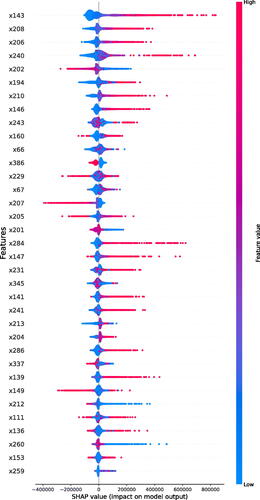
According to the SHAP values, the most influential Variables in the income predictive model (M4) are x143, followed by the variables x208, x206, and x240. From the SHAP summary plot, we notice that as the value of x143 increases, the higher the estimated income of the customers will be. We see this same behavior but in smaller magnitude for the variables x208, x206. On the other hand, we have variables that have a double effect, such as the variable x202, which, if it increases in value, hurts the estimated income, and, if it decreases in value, has a positive effect on the estimated income, with both effects of equal magnitude. We can also observe that there are variables that, when increasing their value, have a negative effect on the estimated income, such as x207 and x149.

These influential explanatory variables have different meanings within the banking institution. In context, the most significant variable (x143) is the maximum amount available in a bank account within a period. The following two most influential variables (x208 and x206) are related to the amounts of customers’ transactional movements. The next variable (x240) relates to the maximum amount available in credit card products. Finally, the variable x202 represents the amounts of transfers made by a customer within 12 months. These variables indicate a customer’s creditworthiness, often associated with their income level.

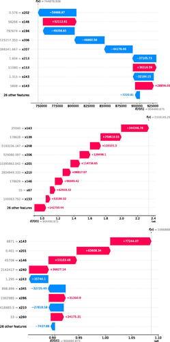
In addition to the global explanation, the ability of the Shapley values to provide local explanations makes it attractive to open the black boxes that are the ML models. To illustrate this, we chose three samples from the test set in which the XGBoost is used to predict income. In Figure 4 we show the contributions of each variable to the model prediction are sorted by their importance (weights). For the first client, variables that contribute negatively to the prediction are x202, x194, x206, x207, x213, and x243. Through them, the model predicts the value $f(x)=744.878\text{CLP}$ from the expected $E[f(x)]=904.490\text{CLP}$. Now, for the second client, all the explanatory variables positively affect the prediction of the model, where the predicted income of this client is $f(x)=\mathrm{2.339.145}\text{CLP}$. Finally, for the last client, the predicted rent $f(x)=\mathrm{1.086.868}\text{CLP}$, where the variables contributing to the increase in the predicted income are x143, x201, and x146. In the three cases, most of these important variables are related to balances and transactions associated with banking products.

Fig. 4 Explanation given by SHAP for three arbitrary clients. This allows to understand how the outcome was achieved. The value of each variable is to the left of equal sign.

4 Discussions and conclusions

The main limitation of this study was the inability to access other databases to measure the effect of our approach on different datasets. Despite this limitation, our findings provide valuable insights into the predictive power of XGBoost models in estimating and predicting the income of bank customers in an anonymous Chilean bank.

Our study demonstrates that appropriate model tuning methods significantly enhance the predictive power of the models. The implementation of the Boruta algorithm and its variant, BorutaSHAP, successfully reduced the number of explanatory variables by approximately 90%. Through our analysis, we determined that the optimal performance was achieved with the BorutaSHAP model using 35 explanatory variables. This reduction not only simplified the model but also reduced training time and data storage requirements, all while maintaining a high level of predictive accuracy.

Additionally, the utilization of SHAP values provided valuable insights for interpreting the results of the complex XGBoost algorithm. The SHAP analysis allowed us to identify the global importance of different variables in predicting income. Our findings revealed that the maximum amount available in a bank account within a given period was the most influential variable. Following that, the customers’ transactional movements and the maximum amount available in credit card products were identified as the next two significant explanatory variables. Lastly, the variable representing the amounts of transfers made by customers within a 12-month period emerged as another important indicator of creditworthiness and income level. Furthermore, at the local level, we employed SHAP to decompose the final predictions of three individual samples into base values and contributions from each variable, providing a detailed understanding of how specific variables influenced the income predictions.

Overall, our study showcases the effectiveness of XGBoost models, the utility of variable selection methods, and the interpretability benefits of utilizing SHAP values in predicting the income of bank customers. While the inability to access additional databases limits the generalizability of our approach, the findings contribute valuable insights for future research and emphasize the potential of machine learning in financial data modeling.

Acknowledgments

We would like to thank anonymous Chilean Bank institution who made this study possible by providing of dataset their customers.

Disclosure statement

No potential conflict of interest was reported by the author(s).

Notes

1 Data science-based analysis techniques come from an interdisciplinary field that employs scientific methods, processes, and systems to extract knowledge and insights from data in various forms. These techniques involve the use of statistical, mathematical, and computational approaches to examine, interpret, and understand datasets.

References

- Alsahaf A, Petkov N, Shenoy V, Azzopardi G. 2022. A framework for feature selection through boosting. Expert Syst Appl. 187:115895.
- Alsaleh N, Farooq B. 2021. Interpretable data-driven demand modelling for on-demand transit services. Transp Res Part A Policy Pract. 154:1–22.
- Ambrey CL, Fleming CM. 2014. The causal effect of income on life satisfaction and the implications for valuing non-market goods. Econ Lett. 123(2):131–134.
- Bergstra J, Yamins D, Cox D. 2013. Making a science of model search: Hyperparameter optimization in hundreds of dimensions for vision architectures. In: International Conference on Machine Learning. PMLR. p.115–123.
- Breiman L. 2001. Random forests. Mach Learn. 45:5–32.
- Burlacu M. 2016. The population’income, expenses and savings as descriptive aspects of the standard of living. Ovidius Univ Ann Series Econ Sci. 16(2):175–180.
- Bussolo M, Davalos ME, Peragine V, Sundaram R. 2018. Toward a new social contract: taking on distributional tensions in Europe and Central Asia. World Bank Publications.
- Cai Q, Abdel-Aty M, Zheng O, Wu Y. 2022. Applying machine learning and google street view to explore effects of drivers’ visual environment on traffic safety. Transp Res Part C: Emerg Technol. 135:103541.
- Chen T, Guestrin C. 2016. Xgboost: A scalable tree boosting system. In: Proceedings of the 22nd ACM SIGKDD International Conference on Knowledge Discovery and Data Mining. p. 785–794.
- Chia G, Miller PW. 2008. Tertiary performance, field of study and graduate starting salaries. Aust Econ Rev. 41(1):15–31.
- Fafoutellis P, Mantouka EG, Vlahogianni EI. 2022. Acceptance of a pay-how-you-drive pricing scheme for city traffic: the case of athens. Transp Res Part A Policy Pract. 156:270–284.
- Fan J, Wang X, Wu L, Zhou H, Zhang F, Yu X, Lu X, Xiang Y. 2018. Comparison of support vector machine and extreme gradient boosting for predicting daily global solar radiation using temperature and precipitation in humid subtropical climates: a case study in china. Energy Convers Manage. 164:102–111.
- Fuders F. 2023. Economic resilience in the face of external shocks. In: How to Fulfil the UN sustainability goals: rethinking the role and concept of money in the light of sustainability. Cham: Springer. p. 327–344
- Futagami K, Fukazawa Y, Kapoor N, Kito T. 2021. Pairwise acquisition prediction with shap value interpretation. J Finance Data Sci. 7:22–44.
- García-Alonso CR, Torres-Jiménez M, Hervás-Martínez C. 2010. Income prediction in the agrarian sector using product unit neural networks. Eur J Oper Res. 204(2):355–365.
- Goldberg LR, Mouti S. 2022. Sustainable investing and the cross-section of returns and maximum drawdown. J Finance Data Sci. 8:353–387.
- Gunning D, Stefik M, Choi J, Miller T, Stumpf S, Yang G-Z. 2019. Xai-explainable artificial intelligence. Sci Robot. 4(37):eaay7120.
- Hughes G. 1968. On the mean accuracy of statistical pattern recognizers. IEEE Trans Inf Theory. 14(1):55–63.
- Jaquart P, Dann D, Weinhardt C. 2021. Short-term bitcoin market prediction via machine learning. Finance Data Sci. 7:45–66.
- Keany E. 2020. Borutashap: A wrapper feature selection method which combines the Boruta feature selection algorithm with Shapley values (Version 1.1). Zenodo.
- Kibekbaev A, Duman E. 2016. Benchmarking regression algorithms for income prediction modeling. Inf Syst. 61:40–52.
- Kursa MB, Rudnicki WR. 2010. Feature selection with the Boruta package. J Stat Soft. 36(11):1–13.
- Ładyżyński P, Żbikowski K, Gawrysiak P. 2019. Direct marketing campaigns in retail banking with the use of deep learning and random forests. Expert Syst Appl. 134:28–35.
- Lang X, Wu D, Mao W. 2022. Comparison of supervised machine learning methods to predict ship propulsion power at sea. Ocean Eng. 245:110387.
- Lazar A. 2004. Income prediction via support vector machine. In: ICMLA. p. 143–149.
- Lin K, Gao Y. 2022. Model interpretability of financial fraud detection by group shap. Expert Syst Appl. 210:118354.
- Lundberg SM, Lee, SI. 2017. A unified approach to interpreting model predictions. Adv Neural Inf Process Syst. 30.
- Lundberg SM, Erion GG, Lee SI. 2018. Consistent individualized feature attribution for tree ensembles. arXiv preprint arXiv:1802.03888.
- Matkowski M. 2021. Prediction of individual income: A machine learning approach. Bryant Online Repository. Rhode Island: Bryant University.
- Miller T. 2017. Explanation in artificial intelligence: insights from the social sciences. Artif Intell. 267:1–38.
- Mokhtari KE, Higdon BP, Başar A. 2019. Interpreting financial time series with shap values. In: Proceedings of the 29th Annual International Conference on Computer Science and Software Engineering. p. 166–172.
- Molnar C. 2020. Interpretable machine learning. Lulu. com.
- Padarian J, McBratney AB, Minasny B. 2020. Game theory interpretation of digital soil mapping convolutional neural networks. Soil. 6(2):389–397.
- Pedregosa F, Varoquaux G, Gramfort A, Michel V, Thirion B, Grisel O, Blondel M, Prettenhofer P, Weiss R, Dubourg V, et al. 2011. Scikit-learn: Machine learning in python. J Mach Learn Res. 12(Oct):2825–2830.
- Pinelis M, Ruppert D. 2022. Machine learning portfolio allocation. J Finance Data Sci. 8:35–54.
- Ross G, Das S, Sciro D, Raza H. 2021. Capitalvx: a machine learning model for startup selection and exit prediction. J Finance Data Sci. 7:94–114.
- Salas P, De la Fuente R, Astroza S, Carrasco JA. 2022. A systematic comparative evaluation of machine learning classifiers and discrete choice models for travel mode choice in the presence of response heterogeneity. Expert Syst Appl. 193:116253.
- Shapley LS. 1953. A value for n-person games. Contrib Theory Games. 2(28):307–317.
- Shin S, Austin PC, Ross HJ, Abdel-Qadir H, Freitas C, Tomlinson G, Chicco D, Mahendiran M, Lawler PR, Billia F, Gramolini A, Epelman S, Wang B, Lee DS. 2021. Machine learning vs. conventional statistical models for predicting heart failure readmission and mortality. ESC Heart Failure 8(1):106–115.
- Silva CAO, Gonzalez-Otero R, Bessani M, Mendoza LO, de Castro CL. 2022a. Interpretable risk models for sleep apnea and coronary diseases from structured and non-structured data. Expert Syst Appl. 200:116955.
- Silva I, Ferreira C, Costa L, Sóter M, Carvalho L, Albuquerque DCJ, Sales M, Candido A, Reis F, Veloso A, et al. 2022b. Polycystic ovary syndrome: clinical and laboratory variables related to new phenotypes using machine-learning models. J Endocrinol Invest. 45:497–505.
- Singh GD, Vig H, Kumar A. 2021. A data visualization approach for predicting the income class of the population. In: 2021 5th International Conference on Electronics, Communication and Aerospace Technology (ICECA). IEEE. p. 1042–1047.
- Smart JC. 1988. College influences on graduates’ income levels. Res High Educ. 29:41–59.
- Swan N. 2006. Problems in dynamic modeling of individual incomes. In: Swedish Conference on Microsimulation, Stockholm. Vol. 20.
- Thomas SL. 2000. Deferred costs and economic returns to college major, quality, and performance. Res High Educ. 41:281–313.
- Trunk GV. 1979. A problem of dimensionality: a simple example. IEEE Trans Pattern Anal Mach Intell. PAMI-1(3):306–307.
- Vythoulkas PC, Koutsopoulos HN. 2003. Modeling discrete choice behavior using concepts from fuzzy set theory, approximate reasoning and neural networks. Transp Res Part C Emerg Technol. 11(1):51–73.
- Wang H, Liu C, Deng L. 2018. Enhanced prediction of hot spots at protein-protein interfaces using extreme gradient boosting. Sci Rep. 8(1):1–13.
- Wu J, Chen X-Y, Zhang H, Xiong L.D, Lei H, Deng S-H. 2019. Hyperparameter optimization for machine learning models based on Bayesian optimization. J Electron Sci Technol. 17(1):26–40.
- Yu D, Liu Z, Su C, Han Y, Duan, X, Zhang, R, Liu, X, Yang, Y, Xu, S. 2020a. Copy number variation in plasma as a tool for lung cancer prediction using extreme gradient boosting (xgboost) classifier. Thorac Cancer. 11(1):95–102.
- Yu GB, Lee D-J, Sirgy MJ, Bosnjak M. 2020b. Household income, satisfaction with standard of living, and subjective well-being. the moderating role of happiness materialism. J. Happiness Stud. 21:2851–2872.