Figures & data
Figure 1. Principle of function of a recirculation well (GCW).
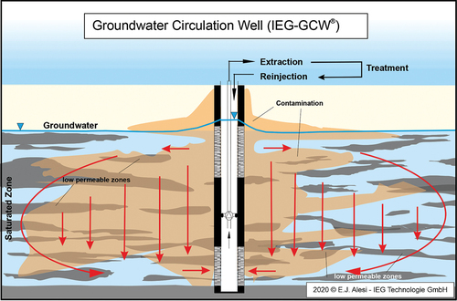
Figure 2. Lithological profile with digitally generated grains.
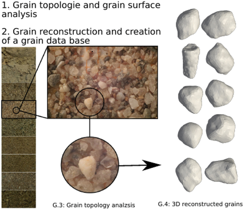
Figure 3. Digitally generated soil layer composed of resolved grains of different size and shape as basic microstructure for numerical analysis (Hötzer et al. Citation2018).
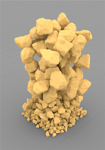
Figure 4. Flow simulation through a sediment of digital grains.
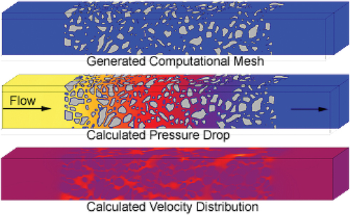
Figure 5. Definition of the mobile and immobile phase (left figure) and the porous region (right figure).
Figure 6. Subsurface lithology for a real heat storage facility in Italy.
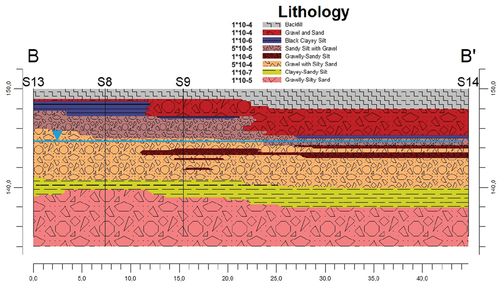
Figure 7. Digitally generated beads with different sizes and alignment.
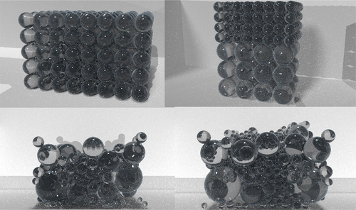
Figure 8. The simulation area. (Top) Total flow area, a porous zone filled by chaotically arranged beads. (Bottom) Dual-porosity approach: generated model with a porous region (green) representing the beads.
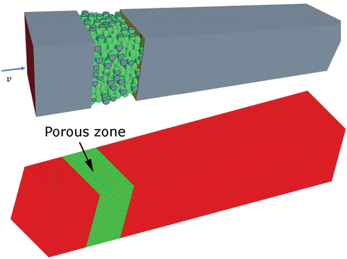
Table 1. Determination of the permeability for the ideal sphere packing.
Table 2. Determination of the permeability for the chaotic sphere packing.
Table 3. Material and simulation parameters for the bowl packings.
Figure 9. Triangular mesh approximating the surface of ideal and chaotic sphere packings.
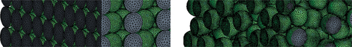
Figure 10. (a) Temporal temperature development in the area for ideal and chaotic sphere packing. (b) Comparison of two solvers: pressure loss in the region for the ideal and chaotic sphere packing.
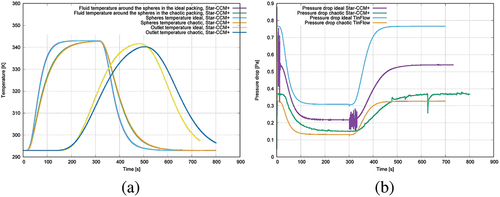
Figure 11. Comparison of two solvers. (a) Temporal temperature development in the region for an ideal sphere packing. (b) Temporal temperature development in the region of chaotic sphere packing.
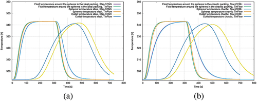
Figure 12. Dimensions and positions of sensors for the experimental set-up.

Figure 13. Experimental set-up.
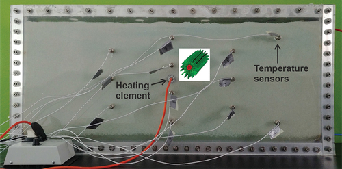
Table 4. Material and simulation parameters for the simulated experiment.
Figure 14. Measured time-dependent temperature for sensor 8 and 5.
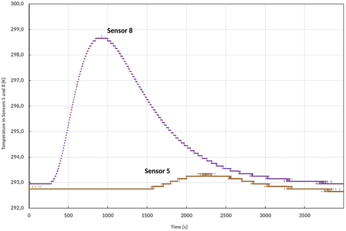
Figure 15. The obtained temperature response at sensor 8. Results of the experiment and simulations with star-CCM+ and TinFlow.
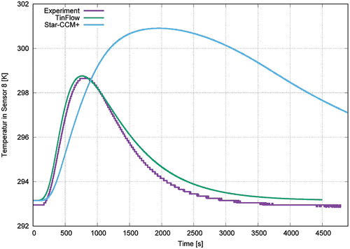
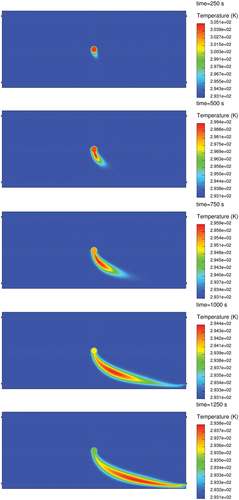
Figure 16. Temperature distribution of a simulation at subsequent time steps in the middle cross-section of the computational domain.