Artificial neural network analysis of the flow of nanofluids in a variable porous gap between two inclined cylinders for solar applications

Figures & data

Figure 1. (a) Geometry (b). Grids.

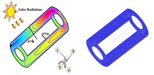
Table 1. Materials’ thermal and physical properties.

Physical Features	Cu	PVA	Water
$k\left(W/\mathrm{mK}\right)$	400	0.2	0.61
$c_p\left(J/\mathrm{Kg}K\right)$	385	2000	4179
$\rho \left(\mathrm{Kg}/m^3\right)$	8933	1020	997
$\text{β}\left(1/k\right)$	1.67	25	21

Figure 2. (a, b): Neural networking adoption for the proposed model.

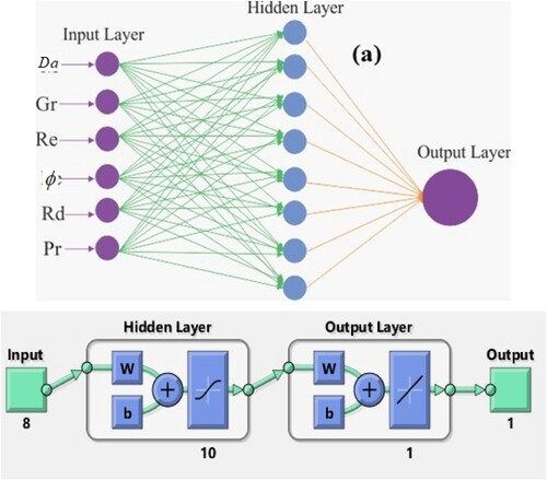
Figure 3. (a-g): $f\left(\eta \right)$VS (a)$\mathrm{Gr}$ (b) AE performance, (c) MSE measures,(d) STs performance (e) EHs performance, (f) fitting curve, (g) performance of the Regression.

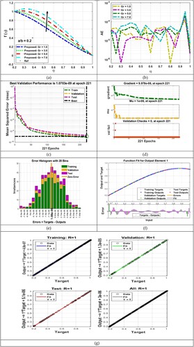
Figure 4. (a-g): $f\left(\eta \right)$VS (a)$\mathrm{Da}$ (b) AE performance, (c) MSE measures,(d) STs performance (e) EHs performance, (f) fitting curve, (g) performance of the Regression.

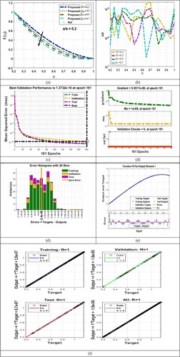
Figure 5. (a-g): $f\left(\eta \right)$VS (a) $\varphi ={\varphi }_1+{\varphi }_2,$ (b) AE performance, (c) MSE measures,(d) STs performance (e) EHs performance, (f) fitting curve, (g) performance of the Regression.

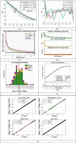
Figure 6. (a-g): $\theta \left(\eta \right)$VS (a) $\mathrm{Rd},$ (b) AE performance, (c) MSE measures,(d) STs performance (e) EHs performance, (f) fitting curve, (g) performance of the Regression.

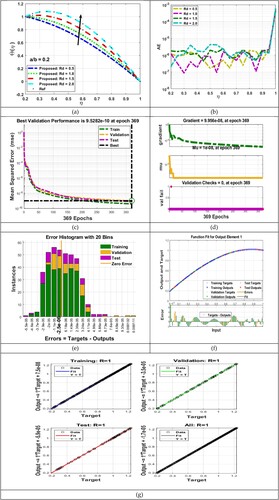
Figure 7. (a-g): $\theta \left(\eta \right)$VS (a) $\varphi ={\varphi }_1+{\varphi }_2,$ (b) AE performance, (c) MSE measures,(d) STs performance (e) EHs performance, (f) fitting curve, (g) performance of the Regression.

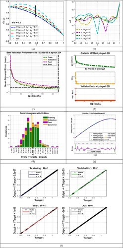
Figure 8. (a-d). Velocity distribution in the variable porous space in terms of the contour.

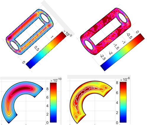
Figure 9. (a,b). (a) Heat transfer rate comparison for $\varphi$ (b) % increase in Heat Transfer.

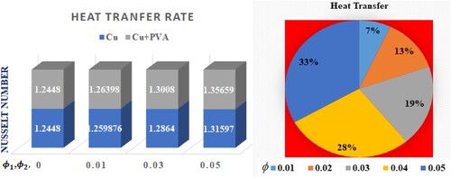
Table 2. Outcomes of LMS-NNA for different scenarios of NCM-HMTMNFF-NNA.

	MSE
Cases	Training	Validation	Testing	Performance	Gradient	Mu	Epoch	Time (s)
I.	$1.345\times {10}^{-9}$	$2.345\times {10}^{-8}$	$3.562\times {10}^{-8}$	$5.632\times {10}^{-9}$	$1.01\times {10}^{-6}$	$1.0\times {10}^{-7}$	1000	02
II.	$3.235\times {10}^{-9}$	$3.321\times {10}^{-9}$	$2.754\times {10}^{-9}$	$6.654\times {10}^{-9}$	$9.87\times {10}^{-8}$	$1.0\times {10}^{-7}$	586	01
III.	$3.432\times {10}^{-8}$	$1.543\times {10}^{-8}$	$5.685\times {10}^{-8}$	$3.673\times {10}^{-8}$	$1.0\times {10}^{-6}$	$1.0\times {10}^{-7}$	486	01
IV.	$4.6542\times {10}^{-10}$	$7.673\times {10}^{-10}$	$4.640\times {10}^{-10}$	$4.784\times {10}^{-10}$	$8.53\times {10}^{-7}$	$1.0\times {10}^{-8}$	897	02
V.	$5.574\times {10}^{-9}$	$5.765\times {10}^{-9}$	$1.046\times {10}^{-8}$	$5.43\times {10}^{-9}$	$1.60\times {10}^{-5}$	$1.0\times {10}^{-8}$	1000	03
VI.	$1.543\times {10}^{-9}$	$1.453\times {10}^{-9}$	$1.453\times {10}^{-9}$	$1.562\times {10}^{-9}$	$5.67\times {10}^{-6}$	$1.0\times {10}^{-7}$	1000	03
VII.	$3.678\times {10}^{-7}$	$2.675\times {10}^{-7}$	$3.321\times {10}^{-7}$	$2.75\times {10}^{-7}$	$3.78\times {10}^{-6}$	$1.0\times {10}^{-5}$	1000	03
VIII.	$3.675\times {10}^{-8}$	$1.648\times {10}^{-8}$	$5.342\times {10}^{-8}$	$3.56\times {10}^{-8}$	$1.32\times {10}^{-5}$	$1.0\times {10}^{-7}$	1000	03

Table 3. The skin friction outputs on the variations of the embedded parameters.

Parameters
$\mathrm{Gr}$	$\mathrm{Da}$	$\varphi ={\varphi }_1+{\varphi }_2$	$C_f$
1	0.1	0.01	2.314782
3			2.305487
5			2.296512
	0.3		2.33187
	0.5		2.354218
		0.03	2.326541
		0.05	2.341871

Table 4. The heat transfer rate versus $\mathrm{Rd}\mathrm{\&}\varphi$.

Acting parameters		Nusselt Number
$\varphi$	$\mathrm{Rd}$	Cu + PVA	Cu
0	0.1	1.2448	1.2448
0.01		1.2639	1.2599
0.03		1.3008	1.2864
0.05		1.35659	1.31597
	0.3	1.25210	1.242531
	0.5	1.27214	1.283214

Table 5. The parameters values range as per stability analysis.

Parameters	Parameters value range as per stability analysis.
$Pr$	For H2O (6.9)
$Pr$	For HNFs (2 to 15)
$\mathrm{Gr}$	1.0 to 7.0 for HNFs
$\mathrm{Da}$	0.1 to 0.7
$\varphi ={\varphi }_1+{\varphi }_2$	0.01 to 0.05
$\mathrm{Rd}$	0.1 to 2.0

Table 6. Based on the common parameter of gap $\eta =\frac{a}{b}$between two cylinders the current work is compared with (Gouran et al., 2022).

Gap	Nusselt Number	Nusselt Number
$\eta =\frac{a}{b}$	Gouran et al. (2022)	Present
0.2	1.45267438926729	1.4527528976154342
0.4	1.5128791062651702	1.5129561342518902
0.6	1.583872901265417	1.58397256431082
0.8	1.647654231289716	1.64775628971652
0.9	2.2356272349082341	2.23684526190245342

Gouran, S., Mohsenian, S., & Ghasemi, S. (2022). Theoretical analysis on MHD nanofluid flow between two concentric cylinders using efficient computational techniques. Alexandria Engineering Journal, 61(4), 3237–3248. https://doi.org/10.1016/j.aej.2021.08.047

 Web of Science ®Google Scholar

Data availability statement

Data will be available on a reasonable request.