Machine learning is coming

KEYWORDS:

• Linear free energy relationships
• machine learning
• LFER

The White Walkers are an ancient humanoid race that was created to protect the Children of the Forest from the First Men but broke free of the Children’s control to become fierce ice creatures that threaten the peoples of Westeros. They do so from beyond the Wall, terrorising these inhabitants with incursions into their territory, all but guaranteeing annihilation if the Wall were to fall. Linear free-energy relationships (LFERs) are ancient methods (relatively speaking) that were created to correlate chemical attributes to reactivity in order to gain insight into mechanisms and guide chemistry investigations. Their utility is seeing a rebirth under the guise of machine learning (ML), which terrorises and intimidates students by using complex mathematical equations and uninterpretable clusters of spots, convoluted branching trees, and wild networks of lines between nodes. This Eric’s Corner is the first of several that will attempt to put machine learning into a historical perspective, to make the field understandable, and to explain those pesky diagrams that so often accompany ML papers. The overarching goal with this series of articles is to show that supramolecular chemistry is a field ripe for application in machine learning. But let us start with some history, and the origins of what is now known as data-driven modelling [1].

In the beginning

Chemistry is a heavily data-driven science, seeking experimental observables to generate trends that explain natural processes at the atomic and molecular level. Correlating data as a tool to gain mechanistic insight into organic chemistry reached a milestone in 1924 when Johannes Nicolaus Brønsted devised a mathematical relationship between acid/base equilibria and rate constants for general acid/base catalysed reactions (Eqs. (1)(1) $log\left(k_{\mathit{obs}}\right)=\mathit{\alpha }\cdot \mathrm{p}{K}_{\mathit{a}\left(\mathit{HA}\right)}+\mathrm{C}$(1) and (2(2) $log\left(k_{\mathit{obs}}\right)=-\mathit{\beta }\cdot \mathrm{p}{K}_{\mathrm{a}\left(\mathit{HB}\right)}+\mathrm{C}$(2) ), respectively) [2]. Equation (1)(1) $log\left(k_{\mathit{obs}}\right)=\mathit{\alpha }\cdot \mathrm{p}{K}_{\mathit{a}\left(\mathit{HA}\right)}+\mathrm{C}$(1) tells us that the rate constant for a general acid (HA) catalysed reaction is related to the acidity of that catalyst (pK_a) via a proportionality constant α (or β for a general base (B) catalysed reaction, using the pK_a of its conjugate acid). If we focus on acid catalysis, the α value tells us the sensitivity of the rate constant to the strength of the acid for a general acid catalysed reaction. If α is zero, the acid catalyst does not affect the rate of the reaction and therefore is not acting in the rate-determining step (rds), i.e. the reaction likely is specific acid catalysed. However, if α is 1, then the strength of the acid catalyst is fully realised in the rds; in other words, the catalyst is considered to have 100% transferred its proton at the transition state (a rare if not impossible occurrence). Similar conclusions can be drawn for values of β in general base catalysis.

(1) $log\left(k_{\mathit{obs}}\right)=\mathit{\alpha }\cdot \mathrm{p}{K}_{\mathit{a}\left(\mathit{HA}\right)}+\mathrm{C}$(1)

(2) $log\left(k_{\mathit{obs}}\right)=-\mathit{\beta }\cdot \mathrm{p}{K}_{\mathrm{a}\left(\mathit{HB}\right)}+\mathrm{C}$(2)

For the purposes of this Eric’s Corner, it is important to note that while the Brønsted relationships were historically used to determine the extents of proton transfer in acid/base catalysis, they can also be used in a predictive fashion. Focusing again on acid catalysis, if α has been determined by experimentally measuring k_obs for several acids of various pK_a values (let us call these acids the ‘training set’), then we can use the resulting linear equation to predict the k_obs for any acid whose pK_a value is known. The equation is a ‘model’ that predicts a structure–reactivity relationship that is univariate, where the pK_a is the ‘feature’ (also called a variable) that modulates the ‘observable’ k_obs. Note the quotation marks used here, hinting that this terminology is going to be important.

The Brønsted equations prompted chemists to explore other ways that parameters describing chemical characteristics could be related to reactivity. The most well-known example is the Hammett plot, named after Louis Plack Hammett [3]. Hammett plots are LFERs that use σ_X values that scale the inductive (and/or resonance) character of substituents X (X = Cl, CH₃, Ph, NO₂, OH, etc., with a different sigma for each X). The σ_X values are derived from the equilibrium acidity constants (K_X) of X-substituted benzoic acids. This scale from electron donating to electron withdrawing substituents correlates to the kinetics (rate constants, k) or thermodynamics (equilibrium constants, K) of any reaction (Eqs. (3)(3) $log\left(k_{\mathrm{X}}/k_{\mathrm{H}}\right)=\mathit{\rho }\cdot {\mathit{\sigma }}_{\mathrm{X}}$(3) and (4(4) $log\left(K_{\mathrm{X}}/K_{\mathrm{H}}\right)=\mathit{\rho }\cdot {\mathit{\sigma }}_{\mathrm{X}}$(4) ), respectively). Note that the correlations are all relative to the substituent being hydrogen. The sensitivity of the rate or equilibrium constants to the σ_X values, relative to their effect on benzoic acid acidity, is reflected by a proportionality constant ρ(rho). Determining ρ for new reactions yields mechanistic information. For example, when the following kinetics (Eq. (3)(3) $log\left(k_{\mathrm{X}}/k_{\mathrm{H}}\right)=\mathit{\rho }\cdot {\mathit{\sigma }}_{\mathrm{X}}$(3) ), a positive or negative ρ value indicates that negative or positive charge is building in a transition state, respectively. It is important to note the generality of this mechanistic probe; it is applicable to many different classes of reactions, far beyond the acid-base reaction of benzoic acid upon which it is based.

(3) $log\left(k_{\mathrm{X}}/k_{\mathrm{H}}\right)=\mathit{\rho }\cdot {\mathit{\sigma }}_{\mathrm{X}}$(3)

(4) $log\left(K_{\mathrm{X}}/K_{\mathrm{H}}\right)=\mathit{\rho }\cdot {\mathit{\sigma }}_{\mathrm{X}}$(4)

But again, for the purposes of this paper, a Hammett plot is also predictive of chemical reactivity. Once a ρ value has been experimentally determined for a new reaction by changing a series of substituents X (the ‘training set’) and using σ_X variables (‘features’) for substituents not in the training set, then either the rate or equilibrium constant ‘observable’ can be predicted for that substituent.

As described, the Hammett σ_X variable reflects electronic effects of a substituent on reactivity, but there are many contributions that make up electronic effects: induction, resonance, hybridisation, field effects, aromaticity, polarisability, etc. It is of interest to get finer details as to the dominant factors of an overall electronic effect. Breaking down the contributions to electronic effects led to the development of multivariate LFERs, which allowed researchers to gain deeper insight into structure–reactivity relationships. For instance, Taft and Topsom expanded to a four-variable approach: field, induction, polarisability, and resonance, each with an associated proportionality constant (Eq. (5)(5) $log\left(k_{\mathrm{X}}/k_{\mathrm{H}}\right)={\rho }_{\mathrm{F}}{\mathit{\sigma }}_{\mathrm{F}}+{\rho }_{\mathrm{x}}{\mathit{\sigma }}_{\mathrm{x}}+{\rho }_{\mathit{\alpha }}{\mathit{\sigma }}_{\mathit{\alpha }}+{\rho }_{\mathrm{R}}{\mathit{\sigma }}_{\mathrm{R}}$(5) ) [4]. Wow, this is getting complicated. Numerous variables, each of which reflects its specific electronic effect for a substituent, with its own specific proportionality constant, are required to generate a multivariate model. Starting to smell like machine learning?

(5) $log\left(k_{\mathrm{X}}/k_{\mathrm{H}}\right)={\rho }_{\mathrm{F}}{\mathit{\sigma }}_{\mathrm{F}}+{\rho }_{\mathrm{x}}{\mathit{\sigma }}_{\mathrm{x}}+{\rho }_{\mathit{\alpha }}{\mathit{\sigma }}_{\mathit{\alpha }}+{\rho }_{\mathrm{R}}{\mathit{\sigma }}_{\mathrm{R}}$(5)

While the univariate LFERs are significant contributions to the field of chemistry, they still come with limitations. They are not able to model chemical reactions where the free energy changes depend upon multiple parameters, not just electronic effects. An important advance occurred in 1952 with the Taft equation (named after Robert W. Taft), that expanded these analyses by incorporating steric effects in addition to electronic effects (Eq. (6)(6) $log\left(k_{\mathrm{s}}/k_{\mathit{CH}3}\right)=\mathit{\rho }\ast \mathit{\sigma }\ast +\mathit{\delta }{E}_s$(6) ). In the Taft approach, there are σ* and E_s structural variables that describe electronic influence and steric size of a substituent (all relative to methyl), and sensitivity parameters ρ* and δ for electronic influence and steric size, respectively. This equation serves as a basis for the paradigm that all chemistry can be explained by electronic and steric effects.

(6) $log\left(k_{\mathrm{s}}/k_{\mathit{CH}3}\right)=\mathit{\rho }\ast \mathit{\sigma }\ast +\mathit{\delta }{E}_s$(6)

Now, with knowledge of σ* and δ gained from a training set, the rate constant for a reaction with substituent S (k_s) can be predicted if σ* and E_s are known for that substituent. The discovery of these mathematical relationships gave chemists a multitude of different options to pick from regarding how to characterise and analyse both new and existing reaction mechanisms. Now, in hindsight, we can also appreciate that these methods were the first inroads into data-driven modelling for predicting chemical reactivity.

In come the machines

The fitting of these linear relationships to derive the proportionality constants (α, ρ, etc.) was done for decades ‘by hand’. The most common approach was the least squares method, which I hope is still taught in middle or high school (I learned how to do this way back in the 1970s!). But of course, nowadays, linear regression and far more complex fitting methods are programmed in computer languages, and the data are contained in a spreadsheet, enabling users to manipulate and process large volumes of data with unprecedented speeds. In turn, this has allowed the field of machine learning to explode with a variety of methods and applications that could not possibly be done by hand. These machines do the fitting with algorithms that minimise the residuals between the experimental data and the computed fit or other measurements of ‘fitness’ such as a loss function. Moreover, in basically all embodiments of ML, the computers vary proportionality constants and mathematical relationships and/or triggers to derive the best fits, just like was done by hand for the early LFERs. Thus, these ‘machines’ have ‘learned’ patterns.

Now that we have stated that the use of a computer to generate a LFER is a simple form of machine learning, let us compare these concepts further by recasting much of the language above into the parlance of ML. An observable is the experimental value that is being sought. For example, the Hammett plot can generate k_X or K_X values once the ρ value for a reaction is known. A model is a mathematical relationship between data and an observable to be predicted. In the examples above, the equations are models. Features are the input variables used to generate the model. In chemistry, each feature is associated with a chemical attribute of the structures used in the training set, e.g. pK_a in a Brønsted plot, σ_X in a Hammett plot, or σ* and E_s in a Taft plot. The training set is the data space that spans the range of values for the features whose observables are known. This is commonly a series of chemical structures whose features are experimentally or computationally derived, and whose desired experimental data has been previously determined. Weights are the learned parameters that map the features onto the observables to be predicted. In the examples above, the weights would be the sensitivity parameters α in a Brønsted plot, ρ in a Hammett plot, or ρ* and δ in a Taft plot. Regression is the process by which a particular algorithm creates the model by learning the weights that best map the training set data onto the experimental observables. The regression can be simple linear regression (deriving univariate or multivariate linear relationships, as with the examples above), nonlinear regression (deriving any function), and/or complex hyperdimensional regression (a function in multidimensional space). Thus, we see that as the regression gets more complex, it becomes worthy of a more fanciful name – machine learning. But the spirit of the analysis is still the same as those from our forefathers Brønsted, Hammett, and Taft.

With the introduction of computers into the field of chemistry also came the ability to computationally generate chemical parameters (features). We no longer need to solely rely on experimentally derived features from training set compounds. For example, electronic structure theory, embodied in ab initio Hartree-Fock or density functional theory, can calculate vibrational frequencies, orbital energy levels, charges on atoms or groups, bond lengths and angles, as well as van der Waals radii (akin to steric size), to be used as features. In fact, the sky is the limit as to what features may be used in ML protocols to make predictions. If inclusion of any feature improves the model, the more the better. One may consider combining σ_X values, with hydrogen bond donating ability of a solvent, with the polarisability of an aromatic ring, or really anything (and I mean any chemical feature), to generate a model. In practice, experimental and calculated features are often combined in a regression routine to generate an accurate model. Each reaction, analytical endeavour, or other chemical analysis require different features and different regression methods to create an optimal model. This resides at the heart of machine learning in chemistry. Especially in the modern day, computer software has become increasingly available and so user-friendly that it has begun to break down the barrier of needing to be a fully trained computational or physical chemist to generate features and models.

An example from our group

Many synthetic methodology chemists now incorporate ML into their everyday routines [5]. The workflow begins with a training set comprised of molecules of interest for their methodology, followed by parameterising those molecules into features derived either from experiment or computation, commonly chosen initially based on the chemical intuition of the chemist. These features are then put through one of many different regression methods to generate models that give an observable of interest, such as a rate constant, a spectroscopic signal, or an enantiomeric excess (ee) value. However, it is uncommon for the calculated observables to be a good fit with the data on the first try. Therefore, this process is iterated numerous times, with tweaks to the training set features and the regression methods, to give a model that best predicts the experimental observable sought.

As an example, let us look at a recent study from our lab. For decades, our group has created rapid assays for determining ee values [6]. We have generated a variety of reversible covalent bonding supramolecular assemblies to bind chiral analytes (alcohols, amines, carboxylic acids, etc.), leading to circular dichroism (CD) signals that can be correlated to ee values. But there is a chicken and egg problem. One needs enantioenriched chiral analytes to generate calibration curves that are used to improve synthetic methods for enantioenrichment of that chiral analyte. Well, would it not be great to have a model that predicts the CD signal, and thereby, the calibration curve of the chiral analyte, obviating the need to enantioenrich that analyte to start? In comes machine learning.

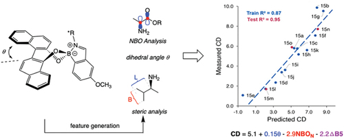
We analysed a boronic acid-based receptor (I love boronic acids!) with a twisted BINOL that reversibly binds chiral primary amines at an o-formyl group (Figure 1). The point chirality of the amine influences the helical chirality of the BINOL, which in turn results in a CD signal. While the details are given in our JACS paper [7], the upshot is that a multivariate linear model reveals that the CD magnitude depends linearly on three features: the twist angle in the BINOL (θ), the natural bond orbital (NBO) charge on the nitrogen, and steric size differences of the groups on the stereocenter of the chiral amine, each with its own weight. Isn’t that cool? Ya gotta luv being a chemist.

Figure 1. A BINOL-based assembly for chiral amine analysis. Features that were important for predicting measured CD were sterics, dihedral angle, and NBO on the nitrogen. This gave a multivariate linear correlation for the CD values and a series of amines (see the JACS paper for details).

The wall has been torn down, but not to fear

With this brief introduction to machine learning, we hope to have laid the foundation for future Eric’s Corners that will explore the details of various ML methods and how they can be used in supramolecular analytical chemistry, as well as make predictions about the future use of ML in supramolecular chemistry generally. The most intimidating factor of ML is getting started and not allowing the fear of the unknown, i.e. the correct features to use, or the best regression method, to hold you back from embracing these powerful predictive tools. The White Walkers have breached the Wall, machine learning has come, so it would benefit us all to learn its ways.

Disclosure statement

No potential conflict of interest was reported by the author(s).

References

- For a more thorough history, see: Williams WL, Zeng L, Gensch T, et al. The evolution of data-driven modeling in organic chemistry. ACS Cent Sci. 2021;7(10):1622–1637. doi: 10.1021/acscentsci.1c00535
- Brønsted J, Pedersen K. Die Katalytische Zersetzung Des Nitramids Und Ihre Physikalisch-Chemische Bedeutung. Z Phys Chem. 1924;108(1):185–235. doi: 10.1515/zpch-1924-10814
- Ritchie CD, Sager WF. An examination of structure-reactivity relationships. In: Cohen S, Streitwieser A, and Taft R, editors. Prog Phys Organic Chem; 1964. pp. 323–400. doi: 10.1002/9780470171813.ch6
- Taft RW, Topsom RD. The nature and analysis of substituent electronic effects. Prog Phys Org Chem. 2007;16:1–83. doi: 10.1002/9780470171950.ch1
- Shi Y-F, Yang Z-X, Ma S, et al. Machine learning for chemistry: basics and applications. Eng. 2023;27:70–83. doi: 10.1016/j.eng.2023.04.013
- Herrera BT, Pilicer SL, Anslyn EV, et al. Optical analysis of reaction yield and enantiomeric excess: a new paradigm ready for prime time. J Am Chem Soc. 2018;140(33):10385–10401. doi: 10.1021/jacs.8b06607
- Howard JR, Bhakare A, Akhtar Z, et al. Data-driven prediction of circular dichroism-based calibration curves for the rapid screening of chiral primary amine enantiomeric excess values. J Am Chem Soc. 2022;144(37):17269–17276. doi: 10.1021/jacs.2c08127