Dual-porosity approach: heat transfer and heat storage processes in porous media

ABSTRACT

This study emphasizes the significance of understanding groundwater flow behavior for effective contaminant transport and heat storage. Aquifers, with their irregular shapes and variable permeability, exhibit anisotropic flow resistances that affect mass and heat transfer, posing challenges for modeling. The dual-porosity model is used as a numerical approach to calculate macroscopic heat transfer without explicitly resolving the structure. By solving equations for mobile and immobile phases and coupling relevant equations for heat conservation, this model was applied to transient numerical experiments simulating heat transfer and storage in a desktop model filled with glass beads. Results indicate alignment with experimental and numerical models resolving porous structures on the microstructure scale. This methodology offers a comprehensive digital toolbox for solving large-scale heat storage problems in aquifers, contributing to digital and sustainability transformations with reasonable computational demands.

KEYWORDS:

• Dual-porosity
• computational fluid dynamics
• adsorption

1. Introduction

Efficient energy usage is a critical challenge that requires effective energy storage solutions. When utilizing renewable energy sources, there is often a delay between energy generation and consumption, making energy storage crucial. Similarly, industrial processes for material production often generate large amounts of thermal energy, which are released into the environment if not recovered (Sommer et al. 2013; Jarullah and Noor 2019; Simons et al. 2021). For example, in gasoline production, the cracking process requires high temperatures and cooling to maintain stable operating conditions, resulting in substantial amounts of low-grade heat. This excess energy can be reused in the form of district heating in winter, but in summer, it is usually wasted. Energy storage systems can enhance energy efficiency by facilitating the storage and utilization of surplus energy (Xu et al. 2014; Dostál and Ladányi 2018).

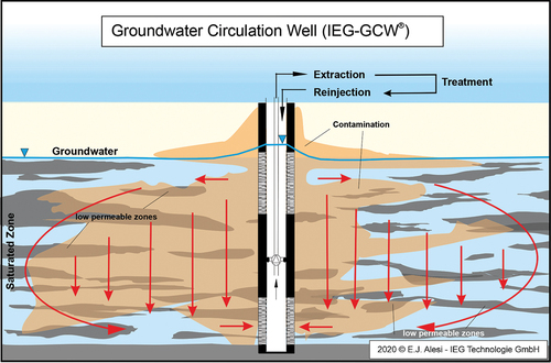
Energy storage can be categorized into short term and seasonal, depending on the duration of storage. While short-term storage lasts only a few days between loading and unloading, long-term storage can last several months. In this context, underground storage facilities are being explored for their huge energy capacity and long-term storage capabilities. For the storage of low-grade heat, appropriate methods for charging and discharging the underground storage system are necessary. The vertical recirculation well method, which involves withdrawing groundwater from one screen section and returning it to another screen section, has proven to be effective for groundwater remediation. This creates a recirculation flow in the subsurface that facilitates continuous heat release to the subsoil. However, the anisotropic stratification of different layers in the subsurface can influence the recirculation flow due to the natural stratification history. This, in turn, leads to anisotropic resistance behaviour that may severely affect the corresponding flow dynamics. As a result, heat transfer to the solid phase in the pore space is also influenced.

An accurate description of the flow process in heterogeneous porous structures is crucial for predicting such heat storage processes. As the subsurface is increasingly becoming a focus for heat storage or heat supply systems, knowledge of sediment particles, their surface properties and spatial structure are essential for a realistic description of fluid transport, energy flows and material changes in the subsurface. All relevant material transformations and mass transfer processes in an aquifer occur at the pore-level scale.

In contrast to the conventional convection–diffusion equation model, the dual-porosity model enables the modelling of fluid dynamics and transport phenomena in porous media with different pore scales, such as natural soils or stratified rocks. The key idea of this model is based on the assumption that the considered porous material can be divided into two distinct domains: a mobile domain, which represents fluid flow (convective transport) through the porous network, and an immobile domain as a stagnation zone, which is essentially characterized by the absence of convection.

In the dual-porosity model, separate sets of equations are used to describe the flow and transport in each of the two domains, and then the equations are coupled to represent the overall behaviour of the system. This approach allows for the calculation of macroscopic properties of porous media, such as effective heat conductivity, heat capacity, etc., without a need for a detailed resolution of the material’s structure at the pore scale.

Dual-porosity models have been widely used in various fields, including hydrology, petroleum engineering and geothermal energy production. They are particularly useful when porous media have complex structures, such as fractured rock or layered sedimentary deposits. By providing a simplified representation of the system, dual-porosity models can help better to understand the behaviour of fluids in such complex environments.

This paper describes the dual-porosity model integrated into the Navier–Stokes solver TinFlow (Kneer 2022) for the numerical description of the flow and heat transport process in porous regions and results of energy storage processes compared to laboratory experiments and numerical simulations at the pore scale. The study is conducted in two steps. First, numerical experiments are carried out using a domain filled with glass beads and digitally reproduced sediments to reconstruct real porous structures. Second, the macroscale calculation results are validated with results obtained from an experimental set-up.

Figure 1 shows the principle of a GCW with two screen sections. This is a well-established technique to solve water treatment or thermal storage issues, which has been successfully applied in several industrial sites for groundwater remediation (Pierro et al. 2017; Zhu et al. 2020). However, there are several unknown factors for the layout and operation of such systems. First, the porous media often contains heterogeneous permeable zones, resulting in an anisotropic flow resistance behaviour (for fracture modelling see (Prajapati et al. 2020)). Second, the saturated zones consist of the stagnation or low-permeability domain characterized by the absence of convection and representing an immobile phase for both storage and release of energy. This process leads to a change of the inner energy within the immobile phase. The circulation pump creates a flow through the pore channel matrix by forced convection. The mobile phase changes its enthalpy during this time-dependent process. Considering a quasi stationary process within a time step directly leads to a strong coupling of advective and conductive processes, whereas the storage capacity of the solid matrix is a damping element in the whole process.

Figure 1. Principle of function of a recirculation well (GCW).

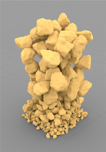
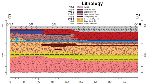
Predicting these dynamic processes requires advanced numerical methods. These days, algorithms are available to resolve grains from sand layers and build digitally reconstructed sediment layers. Figure 2 shows different grain topologies extracted and reconstructed from a soil layer. The reconstructed grains contain information on the effective grain diameter and the topology. Grain reconstruction methods have been developed within the microstructure simulation framework Pace3D to automatically generate digital twins of grains and to establish a grain database. Using physical engines like bullet (bulletphysics.org 2022), those digital twins may be ordered to build a layer of grains that represent at least a digital model of a realistic sand layer. Figure 3 shows a reconstructed layer with representations of different grains.

Figure 2. Lithological profile with digitally generated grains.

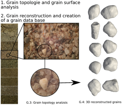
Figure 3. Digitally generated soil layer composed of resolved grains of different size and shape as basic microstructure for numerical analysis (Hötzer et al. 2018).

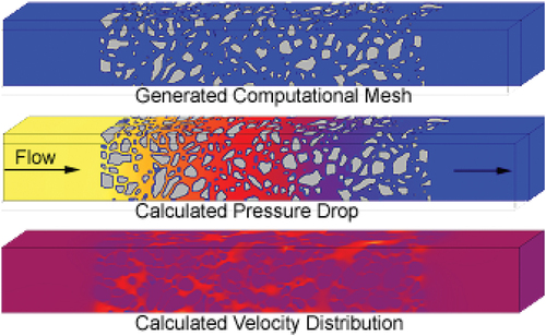
From those digital models, a flow model can be extracted to perform numerical flow simulations on the microstructural pore scale. The resolution of these models requires enormous computational resources if larger volume elements in 3D are considered. The use of such detailed models is limited to either small computational domains or single large-scale simulations. Figure 4 shows an example of a flow simulation through resolved grains using the PACE3D-solver (Hötzer et al. 2018).

Figure 4. Flow simulation through a sediment of digital grains.

Macroscopic models are widely available using the porous region approach. Anisotropic flow behaviour can be implemented by means of tensors to describe the flow resistance in a porous region. When multiple porous regions are combined so that the subsurface layers are reconstructed as composite porous regions, it is evident that the flow behaviour through such combinations is anisotropic (Prajapati et al. 2018). Most of the state-of-the-art Navier–Stokes solvers can compute the anisotropic flow behaviour, but the ‘storage’ capabilities of the immobile phase are not accurately addressed. The problem lies in defining a porous region using effective parameters for the properties. Concerning the viscosity, it is obvious that this property only influences the mobile phase, i.e. the fluid phase. However, concerning thermal properties like heat capacity and heat conductivity, effective parameters have to be defined that are calculated using mass or volume averages. For a stationary operation, which is mostly not the case in groundwater remediation, these effective thermal properties are sufficient. In the case of unsteady heat and mass transfer processes, the unresolved structure of the matrix must be taken into account for simulation. Therefore, the dual-porosity approach as an additional advanced modelling method has to be applied to the porous region.

In the last decades, several investigations using the dual or double porosity approach have already been published. (Toride and Leij 1999) and others (Tayler 1954; Quintard and Whitaker 1994b) worked on flow in porosities under different conditions. (van Genuchten and Wagenet 1989) discussed in his paper a two-site/two-region model which is similar to the dual-porosity approach. Dual-porosity means that the solid portion in a porous region is not resolved as a structure but is modelled as an immobile phase via an additional energy or concentration equation. Structural properties can be represented by incorporating their appropriate effective quantities in this approach. The immobile phase is the storing structure. Between the flow (enthalpy transport) and the immobile phase, heat and mass transfer combined with storing effects have to be accurately computed to get such kind of time-dependent flow simulations. Figure 5 shows a porous region including the mobile (fluid) and immobile (solid) phases.

Figure 5. Definition of the mobile and immobile phase (left figure) and the porous region (right figure).

Recently, the Navier–Stokes solver TinFlow has been extended by the dual-porosity approach for heat and mass transfer. The enhanced CFD-solver TinFlow has been validated by comparison with selected experiments and microstructure simulations of resolved structures.

Based on a validated dual-porosity model using the state-of-the-art CFD-solver TinFlow time-dependent storage process for subsurface storage units can be addressed. The advantage of this method can be summarized as follows:

• Huge subsurface dimensions can be modelled without resolving any grain/sediment structures.

• The computing time for thermal storage processes in seasonal storage scale can be massively reduced.

• Fast prediction to define optimal operational conditions for heat storage from industrial heat waste or other energy resources.

• By parallelizing the solution algorithm, the fluid mechanics calculation (3D) with dual-porosity can be carried out on high-performance clusters or Linux clusters in manageable periods of time.

• The dual-porosity approach is also applicable for other porous systems, and it is usable for any variable porous systems from nature or from industrial applications like membranes, foam structures and textiles.

2. Dual-porosity approach and modelling

The idea of dual-porosity is as follows:

Porous systems are characterized by a complicated internal structure. In order to map large volumes of such a structure, it is therefore necessary to work with high resolution. This goes hand in hand with a very fine grid, which makes it necessary to use an extremely large number of cells. This, in turn, leads to very large memory requirements (several billion cells) and very long simulation times (several decades), which makes efficient numerical analysis impossible.

Dual-porosity solves this problem by dispensing with the resolution of the pore structure. Instead, each cell has both the properties of the solid matrix and the properties of the flowing medium, and each cell is the same in terms of these parameters. This means that fewer cells and less memory are required, and the associated simulation time is therefore much shorter. The modelling of these parameters is explained below.

Porous systems can also be represented by several porous zones with each of them having different porous properties like permeability, porosity, heat conductivity (for fluid and solid), etc., integrated into a flow domain. The flow domain represents therefore a variable porosity media and is therefore anisotropic (as a global porosity) concerning the properties. A typical variable porosity is typically existent for a subsurface formation, which can be seen in Figure 6. The variable porosity approach is implicitly integrated into the TinFlow-solver, treating each porosity is as a subdomain with its (dual) properties. The dual-porosity approach is then applied to each subdomain. It is not limited to one porous zone. The dual-porosity method does not ‘exclude’ a variable porosity model, although a usual variable porosity model does not ‘implicitly’ include a dual-porosity model. For our experimental investigations and numerical calculations, a bed of glass beads has been used (see Section 3). This bed of glass beads represents one porous zone that has been used to study heat propagation processes under dedicated flow conditions. A variable porosity model would not have been useful in this context, but for field tests, it is obligatory and possible to be applied for.

Figure 6. Subsurface lithology for a real heat storage facility in Italy.

Dual-porosity denotes a dual system built from a mobile fluid phase and an immobile phase, which represent the solid particles that are fixed in the space (see Figure 5). As the structure is not resolved in space and time, the solid regions are represented ‘virtually’ to enable accurate computation of the influence of charging and discharging. The porosity of a porous region is defined by

(1) $\mathit{\varphi }=\frac{V_f}{V_t}$(1)

where $V_f$ represents the fluid volume and $V_t$ the total volume (fluid and solid). Thus, porosity is defined as the fluid portion in a given volume. For a porosity of $\mathit{\varphi }=0.34$, only 34% of the total volume $V_t$ is filled with a mobile phase represented by the fluid. Any effective parameters for the given volume cannot accurately represent the storage effects. In the next section, we briefly derive the well-known Darcy law, a simplification of the Navier–Stokes equation. If the flow velocity is very slow, which is typical for silty sand layers, the momentum equation can be reduced in the following way:

(2) $\mathit{K}=\frac{\dot{V}\cdot \mathit{\mu }\cdot \mathit{l}}{\mathrm{\Delta p}\cdot \mathit{A}}\left[\mathrm{\%}\right]\mathrm{with}\mathit{K}\mathrm{permeability}\dot{V}\mathit{\hspace{0.17em}}\mathrm{volume}\mathrm{rate}\mathit{\mu }\mathrm{dynamic}\mathrm{viscosity}\mathit{l}\mathrm{characteristic}\mathrm{length}\mathrm{\Delta }\mathit{p}\mathrm{pressure}\mathrm{difference}\mathit{A}\mathrm{flow}\mathrm{area}$(2)

2.1. Pressure drop in porous materials

To derive Darcy’s law, we assume a very slow flow velocity, which is typical for silty sand layers, and impose it on the momentum equation. The flow-through porous media is always accompanied by pressure loss and energy loss. The determination of the pressure loss is just as important as pipes or other flow components, which contain no porosity. The determination of the permeability has already been dealt with using Equation 2.(2) $\mathit{K}=\frac{\dot{V}\cdot \mathit{\mu }\cdot \mathit{l}}{\mathrm{\Delta p}\cdot \mathit{A}}\left[\mathrm{\%}\right]\mathrm{with}\mathit{K}\mathrm{permeability}\dot{V}\mathit{\hspace{0.17em}}\mathrm{volume}\mathrm{rate}\mathit{\mu }\mathrm{dynamic}\mathrm{viscosity}\mathit{l}\mathrm{characteristic}\mathrm{length}\mathrm{\Delta }\mathit{p}\mathrm{pressure}\mathrm{difference}\mathit{A}\mathrm{flow}\mathrm{area}$(2) The relationship between the flow velocity $\mathit{u}$ through a porosity $\mathrm{\Phi }$ and the applied pressure gradient along the pipe axis can be calculated using Darcy’s law according to Equation 3(3) $\mathit{u}=-\frac{K}{\mu }\frac{\mathrm{\partial p}}{\mathrm{\partial x}}$(3) :

(3) $\mathit{u}=-\frac{K}{\mu }\frac{\mathrm{\partial p}}{\mathrm{\partial x}}$(3)

For an isotropic material, the permeability $\mathit{K}$ is a scalar, and the relationship between the velocity vector $\vec{v}$ and the pressure gradient in the three coordinate directions can be represented as follows:

(4) $\mathrm{\nabla p}=-\frac{\mu }{K}\mathit{v}$(4)

For the average fluid velocity $\mathit{v}=(v_1,v_2,v_3)$ in a porosity, Darcy velocity (Nield and Bejan 2013) can be expressed as follows:

(5) $\mathit{v}=\mathrm{\Phi }\cdot \mathit{V}\mathrm{with}\mathrm{\Phi }\mathit{\hspace{0.17em}}\mathrm{porosity}\mathit{V}\mathrm{velocity}\mathrm{in}\mathrm{the}\mathrm{pores}(\mathrm{fluid})$(5)

The Darcy Equation 4(4) $\mathrm{\nabla p}=-\frac{\mu }{K}\mathit{v}$(4) was verified by numerous experiments over the decades, whereby it should be mentioned that the temperature-dependent viscosity according to the original investigations by Darcy had shown an influence on the results obtained (Nield and Bejan 2013).

Darcy’s correlation only takes into account the viscous term. In a small velocity regime according to (Nield and Bejan 2013), satisfactory agreements with practical experiments are found. However, at higher flow velocities, a non-linear term (inertia term) is to be considered. This extension with the quadratic term goes back to Forchheimer. Eq. 6(6) $\mathrm{\nabla }\mathit{p}=-\frac{\mu }{K}\mathit{v}-\frac{c_f\cdot {\rho }_f}{\sqrt{\mathit{K}}}|\mathit{v}|\mathit{v}\mathrm{with}{c}_f\mathrm{inertial}\mathrm{coefficient}{\rho }_f\mathrm{density}\mathrm{of}\mathrm{the}\mathrm{fluid}$(6) shows the extended correlation reading:

(6) $\mathrm{\nabla }\mathit{p}=-\frac{\mu }{K}\mathit{v}-\frac{c_f\cdot {\rho }_f}{\sqrt{\mathit{K}}}|\mathit{v}|\mathit{v}\mathrm{with}{c}_f\mathrm{inertial}\mathrm{coefficient}{\rho }_f\mathrm{density}\mathrm{of}\mathrm{the}\mathrm{fluid}$(6)

The modification of the Darcy equation was made by Dupuit (1863) and Forchheimer (1901), where $c_f$ depends on the type of porosity and represents a coefficient of inertia. According to Nield and Bejan (2013), the transition from a Darcy flow (Whitaker 1986a) to a Darcy–Forchheimer flow occurs at the permeability Reynolds number $\mathit{R}{e}_K\sim {10}^2$. This is explained by the occurrence of the first eddies. Further literature sources (Summ 2001; Peszynska et al. 2010; Bejan 2013) explain this change based on a laminar–turbulent transition of the flow in the porosity, which takes place at a universal local Reynolds number of $\mathit{Re}\sim {10}^2$.

Another approach to extending the Darcy equation is known as the Brinkmann equation. The Brinkmann equation (see Equation 7(7) $\mathrm{\nabla }\mathit{p}=-\frac{\mu }{K}\mathit{v}+\tilde{\mu }{\mathrm{\nabla }}^2\mathit{v}\mathrm{with}\tilde{\mu }=\frac{\mu }{\mathrm{\Phi }}.$(7) ) uses a viscous term analogous to the Laplace term of the Navier–Stokes equations instead of the inertia term (Durlofsky and Brady 1987; Whitaker 1996; Shi and Wang 2007; Srinivasan and Nakshatrala 2010). Applying the Brinkmann equation is only recommended for porosity values of $\mathrm{\Phi }>0.6$ (Nield and Bejan 2013). The pressure gradient is given by

(7) $\mathrm{\nabla }\mathit{p}=-\frac{\mu }{K}\mathit{v}+\tilde{\mu }{\mathrm{\nabla }}^2\mathit{v}\mathrm{with}\tilde{\mu }=\frac{\mu }{\mathrm{\Phi }}.$(7)

Together with the Navier–Stokes equations, the Darcy–Forchheimer’s equation is one of the most common approaches in standard CFD codes. Further details for an extension of the Forchheimer equation (Forchheimer–Brinkmann correlation) can be found in Vafai and Tien (1981) and Qu et al. (2013), and for the derivation of the Navier–Stokes equations, we refer to Ferziger and Peric (1997), Schlichting and Gersten (2003) and Laurien and Oertel (2003). The Navier–Stokes equations for incompressible flows in an arbitrary coordinate system are written as

(8) $\mathit{\rho }\left(\frac{\mathrm{\partial V}}{\mathrm{\partial t}}+(\mathit{V}\cdot \mathrm{\nabla })\mathit{V}\right)=-\mathrm{\nabla p}+\mathit{\mu }{\mathrm{\nabla }}^2\mathit{V},$(8)

using a symbolic notation.

Taking into account the Darcy–Forchheimer approach (Nield and Bejan 2013; Qu et al. 2013) and the use of the Darcy velocity $\mathit{v}=\mathrm{\Phi }\cdot \mathit{V}$, the modified Navier–Stokes equations for steady and incompressible flows are as follows:

(9) $\frac{\rho }{{\mathrm{\Phi }}^2}(\mathit{v}\cdot \mathrm{\nabla })\mathit{v}=-\mathrm{\nabla p}+\frac{\mu }{\mathrm{\Phi }}{\mathrm{\nabla }}^2\mathit{v}-\frac{\mu }{K}\mathit{v}-\frac{\rho c_f}{\sqrt{\mathit{K}}}(|\mathit{v}|\cdot \mathit{v})$(9)

This extension of the Navier–Stokes equations presented by (Qu et al. 2013) has two additional terms and a modified term on the right-hand side of the classical Navier–Stokes equations. The first term on the right describes the pressure gradient across the porosity, and the second term represents the viscous contribution according to the Brinkmann expansion (see Equation 7(7) $\mathrm{\nabla }\mathit{p}=-\frac{\mu }{K}\mathit{v}+\tilde{\mu }{\mathrm{\nabla }}^2\mathit{v}\mathrm{with}\tilde{\mu }=\frac{\mu }{\mathrm{\Phi }}.$(7) ). The third term on the right includes shear stress by the Darcy approach introduced in Equation 4(4) $\mathrm{\nabla p}=-\frac{\mu }{K}\mathit{v}$(4) , and the fourth term expresses the Forchheimer extension (inertia term).

Usually, in common CFD codes such as Star-CCM+ (CD-adapco 2012), only the Darcy–Forchheimer extension is used. Since large pressure gradients arise across the porosity with relatively large resistances, the convective, viscous, and temporal terms of the momentum equation are negligible, resulting in a reduced momentum equation as given in Eq. 10(10) $\mathrm{\nabla p}=-a_k\cdot \mathit{v}-b_k\cdot |\mathit{v}|\mathit{v}$(10) . This approach represents a combination of a linear term, similar to that of the pressure loss formula for laminar pipe flows, and a non-linear term similar to the pressure loss formula for turbulent pipe flows (Zierep and Bühler 2010).

(10) $\mathrm{\nabla p}=-a_k\cdot \mathit{v}-b_k\cdot |\mathit{v}|\mathit{v}$(10)

The factor $b_k$ denotes an empirical constant for the porous medium and has the unit $\frac{\mathit{kg}}{m^4}$. The factor $a_k=\frac{\mu }{K}$ is the Darcy number with the unit $\frac{\mathit{kg}}{m^3\mathit{s}}$. As a decision criterion for the application of Darcy or Forchheimer’s equation, the permeability Reynolds number $\mathit{R}{e}_K$ can be used. From a value of $\mathit{R}{e}_K>100$, the quadratic term of the Forchheimer equation predominates. As a rule, the permeability $\mathit{K}$ must be experimentally carried out beforehand or be determined numerically.

2.2. Heat transfer in porous materials

Compared to the pure pipe or channel flow with heat transfer, the heat is not only reduced when the flow in porous media is transferred over the lateral surface but also the webs lying in the fluid area. Thus, especially with a highly porous medium, it can be assumed that more heat is transferred due to the enlarged heat-transferring surface. At the same time, the local heat transfer coefficients can be changed by the porous structure (grains, bricks). Let us distinguish between the two model approaches already discussed:

• In the case of the resolution of the porosity using a reconstructed porosity as displayed in Figure 3, these effects are captured when solving the Navier–Stokes equation with the coupled energy and turbulence equations.

• In the case of a porous region model not resolving the structure, a suitable approach is required to compute the convective heat transfer correctly.

(Yang and Vafai 2011) presents an approach for the solution of the convective heat transfer using a two-equation model. This solution model works with an energy conservation equation for the virtual structure and a second energy conservation equation for the fluid. The approach is reminiscent of the dual-porosity method (Barbe and Kneer 2020) for solving the transport of substances through a porous region.

By the analogy of the heat and mass transport equation reading $\dot{q}=-\mathit{\lambda }\frac{\mathit{dT}}{\mathit{dx}}$ and $\dot{J}=-\mathit{D}\frac{\mathit{dc}}{\mathit{dx}}$, the similarity of the thermal conductivity $\mathit{\lambda }$ and the diffusion coefficient $\mathit{D}$ is obvious. Instead of the temperature gradient, the mass flow $\dot{J}$ is defined by the concentration gradient $\frac{\mathit{dc}}{\mathit{dx}}$. (Whitaker 1967) has already dedicated decades to describe the mass transport within homogeneous and inhomogeneous porous structures. There are numerous literature sources for the interested reader (Whitaker 1986a, 1986b; Quintard and Whitaker 1994a, 1997a, 1997b).

The interaction between the fluid and the structure is realized via a local heat transfer coefficient, whereby a heat supply to the mobile region (fluid) or to the immobile region (solid) is realized. This is done numerically using sources or sinks in the respective conservation equation. An analogous approach is presented by (Qu et al. 2013).

A first approach for the resolution of the porosity based on a microstructure model is provided by (Kopanadis et al. 2010) in the form of a study for the convective heat transport in metal foams. The results obtained (effective heat transfer coefficient) are used for validation compared with literature values (e.g., (Hernandez 2005)), achieving a satisfactory match.

Recalling the two-equation approach, (Nield and Bejan 2013) postulates that due to the thermal fluid-structure interaction locally, it may not be assumed that a thermal equilibrium exists. Instead, the fluid temperature $T_f$ and the solid temperature $T_s$ of the porous medium may be different locally. This is commonly referred to as local thermal nonequilibrium (LTNE), sometimes also as lack of thermal equilibrium. According to Yang and Vafai (2011), Nield and Bejan (2013) and Qu et al. (2013), the solid phase can be calculated by

(11) $(1-\mathrm{\Phi })(\mathit{\rho }\mathit{c}{)}_s\frac{\mathrm{\partial }{T}_s}{\mathit{dt}}=(1-\mathrm{\Phi })\mathrm{\nabla }\cdot ({\mathit{\lambda }}_s\mathrm{\nabla }{T}_s)+(1-\mathrm{\Phi })q_s^{{ }^{\prime \prime \prime }}+\mathit{h}(T_f-T_s)$(11)

Furthermore, the following equation applies to the fluid phase:

(12) $(\mathrm{\Phi })(\mathit{\rho }\mathit{c}{)}_f\frac{\mathrm{\partial }{T}_f}{\mathit{dt}}+(\mathit{\rho }\mathit{c})\vec{v}\cdot \mathrm{\nabla }{T}_f=(\mathrm{\Phi })\mathrm{\nabla }\cdot ({\mathit{\lambda }}_f\mathrm{\nabla }{T}_f)+(\mathrm{\Phi })q_f^{{ }^{\prime \prime \prime }}+\mathit{h}(T_s-T_f)$(12)

$\mathrm{with}\left\{\begin{array}{cc}\mathrm{f},\mathrm{s}& \mathrm{index}\mathrm{for}\mathrm{fluid}\mathrm{or}\mathrm{solid}\\ \mathit{\rho }& \mathrm{density}\\ \mathrm{c}& \mathrm{heat}\mathrm{capacity}\\ \mathit{\lambda }& \mathrm{heat}\mathrm{conductivity}\\ \mathrm{T}& \mathrm{temperature}\\ {\mathrm{q}}^{{ }^{\prime \prime \prime }}& \mathrm{heat}\mathrm{sink}\mathrm{or}\mathrm{source}\\ \mathrm{h}& \mathrm{heat}\mathrm{transfer}\mathrm{coefficient}\end{array}\right\}$

Equations 11(11) $(1-\mathrm{\Phi })(\mathit{\rho }\mathit{c}{)}_s\frac{\mathrm{\partial }{T}_s}{\mathit{dt}}=(1-\mathrm{\Phi })\mathrm{\nabla }\cdot ({\mathit{\lambda }}_s\mathrm{\nabla }{T}_s)+(1-\mathrm{\Phi })q_s^{{ }^{\prime \prime \prime }}+\mathit{h}(T_f-T_s)$(11) and 12(12) $(\mathrm{\Phi })(\mathit{\rho }\mathit{c}{)}_f\frac{\mathrm{\partial }{T}_f}{\mathit{dt}}+(\mathit{\rho }\mathit{c})\vec{v}\cdot \mathrm{\nabla }{T}_f=(\mathrm{\Phi })\mathrm{\nabla }\cdot ({\mathit{\lambda }}_f\mathrm{\nabla }{T}_f)+(\mathrm{\Phi })q_f^{{ }^{\prime \prime \prime }}+\mathit{h}(T_s-T_f)$(12) are describing the energy equations, including the energy transfer between fluid and solid, via a heat transfer coefficient $\mathit{h}$. This last term is coupling the two energy conservation equations. The first terms are the change terms, and there are the conduction terms (2nd term in Equation 11(11) $(1-\mathrm{\Phi })(\mathit{\rho }\mathit{c}{)}_s\frac{\mathrm{\partial }{T}_s}{\mathit{dt}}=(1-\mathrm{\Phi })\mathrm{\nabla }\cdot ({\mathit{\lambda }}_s\mathrm{\nabla }{T}_s)+(1-\mathrm{\Phi })q_s^{{ }^{\prime \prime \prime }}+\mathit{h}(T_f-T_s)$(11) and 3r(3) $\mathit{u}=-\frac{K}{\mu }\frac{\mathrm{\partial p}}{\mathrm{\partial x}}$(3) d term in Equation 12)(12) $(\mathrm{\Phi })(\mathit{\rho }\mathit{c}{)}_f\frac{\mathrm{\partial }{T}_f}{\mathit{dt}}+(\mathit{\rho }\mathit{c})\vec{v}\cdot \mathrm{\nabla }{T}_f=(\mathrm{\Phi })\mathrm{\nabla }\cdot ({\mathit{\lambda }}_f\mathrm{\nabla }{T}_f)+(\mathrm{\Phi })q_f^{{ }^{\prime \prime \prime }}+\mathit{h}(T_s-T_f)$(12) , the convection term for fluid (2nd term in Equation 12(12) $(\mathrm{\Phi })(\mathit{\rho }\mathit{c}{)}_f\frac{\mathrm{\partial }{T}_f}{\mathit{dt}}+(\mathit{\rho }\mathit{c})\vec{v}\cdot \mathrm{\nabla }{T}_f=(\mathrm{\Phi })\mathrm{\nabla }\cdot ({\mathit{\lambda }}_f\mathrm{\nabla }{T}_f)+(\mathrm{\Phi })q_f^{{ }^{\prime \prime \prime }}+\mathit{h}(T_s-T_f)$(12) ) and local sources and sinks. In the absence of phase transitions, chemical reactions, radiation, etc., no other terms need to be considered. Thermal equilibrium between fluid and solid (porous) media is requiring no net flow of thermal energy between fluid and solid. From Equations 11(11) $(1-\mathrm{\Phi })(\mathit{\rho }\mathit{c}{)}_s\frac{\mathrm{\partial }{T}_s}{\mathit{dt}}=(1-\mathrm{\Phi })\mathrm{\nabla }\cdot ({\mathit{\lambda }}_s\mathrm{\nabla }{T}_s)+(1-\mathrm{\Phi })q_s^{{ }^{\prime \prime \prime }}+\mathit{h}(T_f-T_s)$(11) and 12(12) $(\mathrm{\Phi })(\mathit{\rho }\mathit{c}{)}_f\frac{\mathrm{\partial }{T}_f}{\mathit{dt}}+(\mathit{\rho }\mathit{c})\vec{v}\cdot \mathrm{\nabla }{T}_f=(\mathrm{\Phi })\mathrm{\nabla }\cdot ({\mathit{\lambda }}_f\mathrm{\nabla }{T}_f)+(\mathrm{\Phi })q_f^{{ }^{\prime \prime \prime }}+\mathit{h}(T_s-T_f)$(12) , this is only the case if solid temperature $T_s$ is equal to fluid temperature $T_f$. In general, this can locally not be expected. It may happen depending on flow and other environmental conditions, though.

However, the heat transfer coefficient $\mathit{h}$ in the above two energy conservation equations is unknown. Often values from correlations (from experiments) are used. For Reynolds numbers $\mathit{R}{e}_{\mathit{dp}}>100$ (based on the pore diameter $d_p$), a Nusselt correlation (Nield and Bejan 2013) can be specified, which can be used to calculate the heat transfer coefficient. This assumes that the pore diameter is known or that it is a ‘typical’ porosity, such as metal foam. In the case of underground sediments and the occurring heat transfer between fluid and grains, these correlations from (Nield and Bejan 2013) cannot be applied to the dual-porosity model.

The volumetric heat transfer coefficient $\mathit{h}$ connects the fluid and the solid phase. Its dimension is $\frac{W}{m^3\mathit{K}}$, and $\mathit{h}$ is depending on the local fluid velocity $\mathit{u}$. We estimate the heat transfer coefficient, including correlation for the surface area heat transfer coefficient $\mathit{\alpha }$ resp. Nusselt number $\mathrm{Nu}=\frac{\mathit{\alpha }\cdot d}{{\mathit{\lambda }}_f}$ for particles (spheres) in fluidized packed beds and a characteristic length L.

Such a correlation is, for example, contained in (Vdi 2006)[Gj]. However, (Kunii and Suzuki 1967) reported experiments showing much (by magnitudes) smaller Nusselt numbers for small Peclet numbers Pe=Re$\cdot$Pr (i.e. small velocities $\mathit{u}$).

By linearly interpolating their experimental values (see [43, Figure 4]) between the points (Pe = 36, Nu = 10) and (Pe = 0.032, Nu=$1\cdot {10}^{-4}$) plotting the data with double log scales, we derive the correlation 13.

(13) $\mathrm{Nu}=0.02844\cdot \mathrm{P}{\mathrm{e}}^{1.636}\mathrm{for}0.032\le \mathrm{Pe}\le 36$(13)

Comparing the definition of $\mathit{\alpha }$ and $\mathit{h}$, we get $\mathit{L}=\frac{\mathit{\alpha }}{h}=\frac{V}{A}$, where $\mathit{V}$ is the volume (solid and fluid) and $\mathit{A}$ is the surface area involved in heat transfer between solid and fluid. For a packed bed of spheres of radius $\mathit{r}$ and porosity $\mathrm{\Phi }$, we obtain

(14) $\mathit{L}=\frac{r}{3}\cdot \frac{1}{1-\mathrm{\Phi }}$(14)

so that

(15) $\mathit{h}=\frac{\mathit{\alpha }}{L}=\mathrm{Nu}\cdot \frac{{\mathit{\lambda }}_f}{\mathit{L}\cdot \mathit{d}}.$(15)

Instead of using a fixed average value of $\mathit{h}$ and the assumption of an average flow velocity $\mathit{u}$ in the fluid domain, we define a function $\mathit{h}=\mathit{h}(\mathit{u})$, depending on the local flow velocity in each discretization cell. If the range of local velocities is large, the range of Nusselt and $\mathit{h}$ values might be even larger, and the numerical simulation might diverge due to very large heat exchanges in each time step. Applying an upper limit for $\mathit{h}$ solves this problem (e.g. all of our simulations with $\mathit{h}<500000$ converged).

3. Dual-porosity validation methods

With regard to its prediction accuracy during transient energy transport in porous media, the dual-porosity solution method was validated by applying the following methods:

• Numerical study of resolved porosity (glass beads) on the pore-scale as a numerical experiment.

• Experimental set-up using glass beads as porous media.

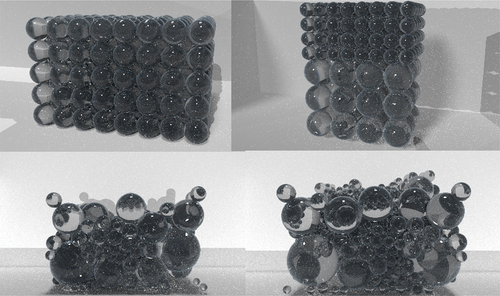
The numerical experiment has the advantage that the bowl packing can be exactly defined by a filling algorithm of the glass beads so that the porous system can be designed as fully isotropic or anisotropic, see Figure 7. We used two different packings of same size spheres: an ideal packing (regularly ordered spheres) and a chaotic packing (irregularly ordered spheres), see Figure 9. Also, within these numerical experiments, any boundary condition can be applied and quickly recomputed. For both experimental studies, a dual-porosity model has been set up, as demonstrated in the next sections.

Figure 7. Digitally generated beads with different sizes and alignment.

3.1. Dual-porosity parameters for ideal and chaotic glass beads (sphere) packing

Several correlations exist for the pressure loss $\mathrm{\Delta p}$ of flows through packed beds of length $\mathit{L}$ of particles or spheres. Well known is the Ergun Eq (Vdi 2006), employing the hydraulic diameter $d_s$ of the particles or spheres:

(16) $\frac{\mathrm{\Delta p}}{L}=\frac{150\cdot \mu }{d_s^2}\cdot \frac{{(1-\mathrm{\Phi })}^2}{{\mathrm{\Phi }}^3}\cdot \mathit{u}+\frac{1.75\cdot \mathit{\rho }}{d_s}\cdot \frac{1-\mathrm{\Phi }}{{\mathrm{\Phi }}^3}\cdot u^2$(16)

Ignoring the right summand in Eq. 16(16) $\frac{\mathrm{\Delta p}}{L}=\frac{150\cdot \mu }{d_s^2}\cdot \frac{{(1-\mathrm{\Phi })}^2}{{\mathrm{\Phi }}^3}\cdot \mathit{u}+\frac{1.75\cdot \mathit{\rho }}{d_s}\cdot \frac{1-\mathrm{\Phi }}{{\mathrm{\Phi }}^3}\cdot u^2$(16) for small velocities $\mathit{u}$ (laminar flow) and comparing to the Darcy equation Eq. 3(3) $\mathit{u}=-\frac{K}{\mu }\frac{\mathrm{\partial p}}{\mathrm{\partial x}}$(3) , we deduce the Kozeny equation

(17) $\mathit{K}=\frac{d_s^2}{150}\cdot \frac{{\mathrm{\Phi }}^3}{{(1-\mathrm{\Phi })}^2}$(17)

It gives the permeability $\mathit{K}$ as a function of geometric parameters only. For spheres of diameter $d_s=1.3\mathrm{mm}$, this expression gives $\mathit{K}=2.23\cdot {10}^{-9}{\mathrm{m}}^2$ for a porosity of $\mathrm{\Phi }=0.41$ (ideal packing) resp. $\mathit{K}=4.85\cdot {10}^{-9}{\mathrm{m}}^2$ for a porosity of $\mathrm{\Phi }=0.485$ (chaotic packing).

More recent is the Molerus correlation (for the formula, see (Vdi 2006)). For the same spheres, it gives $\mathit{K}=2.45\cdot {10}^{-9}{\mathrm{m}}^2$ ($\mathrm{\Phi }=0.41$) resp. $\mathit{K}=5.78\cdot {10}^{-9}{\mathrm{m}}^2$ ($\mathrm{\Phi }=0.485$). These values of the permeability serve as input parameters for the TinFlow simulations, where the resistance factor $\frac{\mu }{K}$ is one of the quantities describing the pressure drop for a given porosity. For an imposed velocity of $\mathit{u}=2.29\cdot {10}^{-4}\mathrm{m}ker$, the Molerus correlation predicts pressure losses of $\mathrm{\Delta }\mathit{p}=0.76$ Pa ($\mathrm{\Phi }=0.41$) resp. $\mathrm{\Delta }\mathit{p}=0.32$ Pa ($\mathrm{\Phi }=0.485$). These pressure losses are exactly reproduced by the TinFlow simulations.

To determine the geometric parameter (permeability $\mathit{K}$), stationary simulations with Star-CCM+ were carried out in the resolved spherical region. The flow through an area, as shown in Figure 8, was simulated for four different velocities $\mathit{u}$ and under constant area and boundary temperature. The calculated pressure drop of the simulations provides the permeability $\mathit{K}$ using the following formula: $\mathit{dp}=\mathit{u}\cdot \mathit{L}\cdot \frac{\mu }{K}$, where $\mathit{dp}$ is the pressure loss, $\mathit{u}$ the inflow velocity, $\mathit{\mu }=0.0010016\mathrm{Pa}\cdot \mathrm{s}$ is the dynamic viscosity of water.

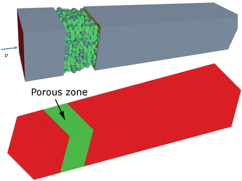
Figure 8. The simulation area. (Top) Total flow area, a porous zone filled by chaotically arranged beads. (Bottom) Dual-porosity approach: generated model with a porous region (green) representing the beads.

The mean value for the permeability of the ideal sphere packing is $3.4502\cdot {10}^{-9}{\mathrm{m}}^2$, and the mean value for the chaotic sphere packing is $4.9269\cdot {10}^{-9}{\mathrm{m}}^2$. The individual values are presented in Tables 1 and 2.

Table 1. Determination of the permeability for the ideal sphere packing.

Velocity	Pressure drop	Permeability $\mathit{K}$
in $\mathrm{m}-0.1\mathit{em}-0.15\mathit{em}\mathrm{s}$	in $\mathrm{Pa}$	in ${\mathrm{m}}^2$
0.000229	0.539	$3.4575\cdot {10}^{-9}$
0.000458	1.080	$3.4511\cdot {10}^{-9}$
0.000687	1.621	$3.4490\cdot {10}^{-9}$
0.000916	2.165	$3.4431\cdot {10}^{-9}$

Table 2. Determination of the permeability for the chaotic sphere packing.

Velocity	Pressure drop	Permeability $\mathit{K}$
in $\mathrm{m}-0.1\mathit{em}/-0.15\mathit{em}\mathrm{s}$	in $\mathrm{Pa}$	in ${\mathrm{m}}^2$
0.000229	0.380	$4.9081\cdot {10}^{-9}$
0.000458	0.757	$4.9236\cdot {10}^{-9}$
0.000687	1.127	$4.9590\cdot {10}^{-9}$
0.000916	1.513	$4.9269\cdot {10}^{-9}$

3.2. Simulations on the pore scale and comparison with the dual-porosity results

For the validation of the dual-porosity model of TinFlow, high-resolution simulations of the flow-through bowl packings were carried out utilizing the resolved digital bead packages with Pace3D and Star-CCM+ to evaluate the flow properties.

Two cut-outs from glass bowl fillings (ideal packing and chaotic packing) were simulated. The individual spherical beads, which were surrounded by water, were modelled as non-moving solid phase. The inflow velocity was assumed to be $2.29\cdot {10}^{-4}\mathrm{m}-0.1\mathit{em}/-0.15\mathit{em}\mathrm{s}$ as a boundary condition. The inflow temperature was chosen to be 70°C for the first $300\mathrm{s}$ and 20°C afterward. The sphere diameter was set to $1.3\mathrm{mm}$. Material data of water were used as a function of temperature. Adiabatic (isolating) temperature boundary condition was assigned to the walls. The fabric and geometry parameters and boundary conditions are summarized in Table 3. Two different porosities have been modelled, resolving the structure and with the dual-porosity approach (porous region). For the resolved model, the fluid domain surrounding the glass beads and the glass beads themselves have been integrated into the computational domain. The flow resistance for the dual-porosity simulation has been taken from Table 1 for the ideal glass beads packing and from Table 2 for the chaotic glass beads packing.

Table 3. Material and simulation parameters for the bowl packings.

Thermal conductivity of glass	$1.129\mathrm{W}-0.1\mathit{em}/-0.15\mathit{em}\mathrm{mK}$
Density of glass	$2500\mathrm{kg}-0.1\mathit{em}/-0.15\mathit{em}{\mathrm{m}}^3$
Heat capacity of glass	$1329\mathrm{J}-0.1\mathit{em}/-0.15\mathit{em}\mathrm{kgK}$
Size of the sphere area	12.35 mm
(height $\times$ width $\times$ length	$\times$ 12.35 mm
in the flow direction)	$\times$ 8.125 mm
Length of the flow inlet	8.775 mm
Length of the flow follow-up	50 mm
Porosity of the ideal packing	0.410
Porosity of chaotic packing	0.485
Initial temperature (water and glass)	20°C
Inlet temperature (for 300 s)	70°C
Inlet velocity (water)	0.229 $0.5\mathit{ex}\mathrm{mm}-0.1\mathit{em}/-0.15\mathit{em}\mathrm{s}$
Timestep	0.1 s

To get a better impression of how beads can be ordered in a computational domain, some examples of digitally generated beads are shown in Figure 7. The digital beads are represented by a triangulated surface mesh, which can be subtracted from a computational domain to get the flow domain. This boolean operation allows generating of both flow domain and immobile phase of the beads. By combining the ‘solid’ domain and the fluid domain, a volumetric computational mesh can be generated for CFD-solver applications. For the validation purpose of the dual-porosity approach, the computational domain consists of a channel with differently ordered and resolved beads inside.

Figure 8 illustrates the total simulation area. The fluid phase around the beads is hidden to enable a view inside the beads. Two kinds of packings are realized: chaotically ordered beads to address an anisotropic behaviour and ideally aligned beads for isotropic flow resistance.

Figure 9 shows sections of the ideal and chaotic sphere packing with its triangulated surfaces. The computational domain of the TinFlow-model with the porous region is shown in Figure 8. The area with the beads is defined by a porous region for which the dual-porosity model is activated. The simulation for this macroscopic model was performed with the same boundary and initial conditions as the simulations with the resolved beads.

Figure 9. Triangular mesh approximating the surface of ideal and chaotic sphere packings.

The temporal mean temperature of the glass spheres and the surrounding water as well as the pressure drop between the inlet and the outlet were evaluated. The determined quantities from simulation data analysis are summarized in Figure 10. Strong oscillations occur at times in the StarCCM+ simulation results for the pressure drop. This may be due to numerical instabilities in the resolved model at singular points, for example where two spheres meet.

Figure 10. (a) Temporal temperature development in the area for ideal and chaotic sphere packing. (b) Comparison of two solvers: pressure loss in the region for the ideal and chaotic sphere packing.

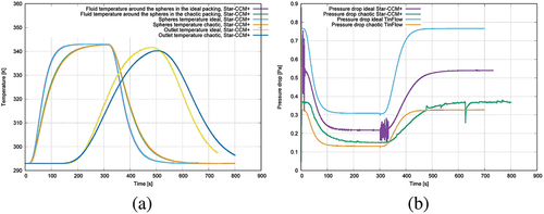
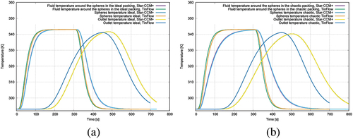
The evaluated values were used to validate the dual-porosity method in the TinFlow solver from TinniT Technologies GmbH. The results show an excellent agreement with the results of the computation using the resolved beats using StarCCM+ (see Figure 11). Figures 10 and Figure 11 show the computed time-dependent temperature and pressure development for simulations performed with the dual-porosity approach (TinFlow) and with resolved glass beads (StarCCM+, see Figure 8). To address the heat storage and the flow resistance in an accurate way, the fluid properties have been modelled for both cases in a temperature dependent way (polynomial for viscosity, density, heat conductivity, heat capacity)), whereas the viscosity is influencing the flow resistance. Two porosities have been modelled and computed (ideal and chaotic packings) with identical boundary conditions. Figure 10(a) shows the simulated results using the two porosities and with resolved glass beads (fluid structure interaction). The computed temperature development does not show significant differences between the chaotic and ideal glass beads packing (StarCCM+). In Tables 1 and 2, the computed permeability for those two porosities is presented. They have been used for the thermal simulations. Figure 10(b) shows the pressure drop computed for those two porosities with resolved glass beads (StarCCM+) and with the dual-porosity approach (TinFlow). The pressure drop computed with those two modelling technologies shows a better accordance in case of the chaotic packing of the glass beads. Figure 11 shows the time-dependent temperature development for both solvers and both porosities. The dual-porosity delivers a very good agreement compared to the results achieved using resolved structures. In addition, the computation takes only 15 min compared to nearly 2 days for the model with resolved structures.

Figure 11. Comparison of two solvers. (a) Temporal temperature development in the region for an ideal sphere packing. (b) Temporal temperature development in the region of chaotic sphere packing.

4. Numerical study and comparison to experimental results

In this section, we describe simulations of heat transport in the numerically replicated test rig from Section 4.1 to validate the models on a macroscopic metre scale using the experiment. Moreover, we investigate mass and heat transport on a much smaller scale (pore-scale) in numerically simulated spherical bulk materials to compare the considered solvers. The underlying model used for the numerical study consists of three domains, as displayed in Figure 12:

Figure 12. Dimensions and positions of sensors for the experimental set-up.

• Porous region (representing the area with glass beads)

• The heater element in the centre of the porous region (made from aluminium)

• Heat distribution element to increase the heat exchanging surface (made from aluminium)

4.1. Experimental set-up

To analyse heat transfer processes in porous media, a dedicated experimental set-up was developed to measure the temperature development in groundwater circulation. The front sides of the set-up consist of two d = 10 mm Plexiglas® (AXT-100-TRAEVO) plates fixed on aluminium profiles (AlMgSi0.5). The aluminium profiles fix the plexiglass plates at a distance of $\mathit{s}=40\mathrm{mm}$. The length of the model is $\mathit{L}=106\mathrm{cm}$. The total inner volume of around $42.3\mathrm{l}$ was filled with $1.0-1.3\mathrm{mm}$ diameter glass beads (SiLibeads type S) to simulate the porous medium. The design of the experimental set-up is shown in Figure 12.

The glass bead characteristics are as follows: bulk density = $1.51\mathrm{kg}-0.1\mathit{em}/-0.15\mathit{em}\mathrm{d}{\mathrm{m}}^3$, porosity = 0.40, and hydraulic conductivity (k-value) = $4\cdot {10}^{-3}\mathrm{m}-0.1\mathit{em}/-0.15\mathit{em}\mathrm{s}$. To establish confined conditions (< 300 Pa), the model was covered and sealed with an aluminium profile. Both small exterior model sides are equipped with three inlet/outlet valves. To protect the circulation pump against carrying glass beads, screw-in sintered bronze filters were applied. The thermal signal was recorded with four-wire technology PFA-encapsulated Pt100 probes with a nominal diameter of $2.1\mathrm{mm}$ (type HSRTD-3-100-A-2 M, manufacturer OMEGA Engineering 73,592 Deckenpfronn/Germany).

The probes have tolerance class A (DIN EN 60,751), which corresponds to a temperature deviation of 0.35 K from the absolute value for a measured value range of 273 K to 373 K. In the plexiglass R front, 12 thermocouples are placed through sealed threaded holes. The signal was recorded in the middle between the two walls. The detailed instrumentation and the dimension of the test facility are shown in Figure 13. Additional probes record the influent and effluent temperature of the water and the room temperature.

Figure 13. Experimental set-up.

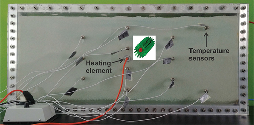
The data reading and storage were performed with modules from WAGO Kontakttechnik (32423 Minden/Germany) with additional real-time visualization to control the measurement processes. An ohmic heating element (heating cartridge, diameter $8\mathrm{mm}$, length $125\mathrm{mm}$) with a heating capacity of $160\mathrm{W}$ was placed in the centre of the model. To optimize the heat transfer into the surrounding saturated porous media, the cartridge was surrounded by a star-shaped array of heat sinks (Fischer SK 620).

The power consumption could be regulated by a phase control unit (10–230 V). A piston pump (manufactured by IEG) connected with a small air compressor was selected for groundwater circulation to prevent a heat increase in water temperature.

The measuring program included the following experiments: The 25 measuring cycles had sampling rates of 1 s each and lasted between 2.5 and 4.0 h, depending on the energy input. When the outlet temperature from the model permanently reached the same value as at the beginning of the operation, the trial was stopped.

4.2. Simulation of the energy transport for the experimental set-up

For the numerical experiments, the following software packets were used: Star-CCM+, a commercial CFD solver from Siemens and TinFlow, the dual-porosity solver developed at TinniT Technologies GmbH.

The simulations at the metre scale are based on the experiments on the rig described in Section 4.1. Figure 12 shows the geometrical dimensions of the experimental set-up. In Table 4, the material/simulation properties and boundary conditions used for the simulations are summarized. In the first 200 s, heat is released by the heater element (60 W). After this period, the heater was switched off. The inlet and outlet of the flow are shown in Figure 12. The recirculation of water has been activated on the right side. Therefore, the generated heat was released to the glass beads surrounded by the water around the cooler element during activated flow recirculation.

Table 4. Material and simulation parameters for the simulated experiment.

Thermal conductivity of glass	$1.06\mathrm{W}-0.1\mathit{em}/-0.15\mathit{em}\mathrm{mK}$
Density of glass	$2500\mathrm{kg}-0.1\mathit{em}/-0.15\mathit{em}{\mathrm{m}}^3$
Heat capacity of glass	$1329\mathrm{J}-0.1\mathit{em}/-0.15\mathit{em}\mathrm{kgK}$
Thermal conductivity of heater (steel)	$58\mathrm{W}-0.1\mathit{em}/-0.15\mathit{em}\mathrm{mK}$
Density of heater (steel)	$7800\mathrm{kg}-0.1\mathit{em}/-0.15\mathit{em}{\mathrm{m}}^3$
Heat capacity of heater (steel)	$460\mathrm{J}-0.1\mathit{em}/-0.15\mathit{em}\mathrm{kgK}$
Thermal conductivity of cooler (Al)	$221\mathrm{W}-0.1\mathit{em}/-0.15\mathit{em}\mathrm{mK}$
Density of cooler (Al)	$2700\mathrm{kg}-0.1\mathit{em}/-0.15\mathit{em}{\mathrm{m}}^3$
Heat capacity of cooler (Al)	$920\mathrm{J}-0.1\mathit{em}/-0.15\mathit{em}\mathrm{kgK}$
Timestep	1 s
Physical duration of the simulation	120 min
Inflow velocity	$0.368391\mathrm{m}-0.1\mathit{em}/-0.15\mathit{em}\mathrm{s}$
Initial temperature of the system	20°C

The flow region is filled with glass spheres with a diameter of $1.3\mathrm{mm}$.

In Star-CCM+, the area where the flow was simulated was modelled as a homogenized porous region with a constant porosity of $\mathrm{\Phi }=0.4$. The values for porous viscous resistance were chosen anisotropically to $172365\mathrm{kg}-0.1\mathit{em}/-0.15\mathit{em}\mathrm{m}3\cdot \mathrm{s}$ perpendicular to the direction of gravity and $455040\mathrm{kg}-0.1\mathit{em}/-0.15\mathit{em}\mathrm{m}3\cdot \mathrm{s}$ parallel to the direction of gravity because the spheres ‘settle’ under the effect of gravity, i.e. they become denser in the downward direction.

Transient CFD simulation was carried out by considering a laminar flow.

In the ‘Heater’ region, Volumetric Heat Source is selected as the boundary condition. The water flows in through the upper right inlet (Velocity Inlet boundary condition) and is pumped out at the lower right outlet (Pressure Outlet boundary condition) so that the inflow velocity is $0.368391\mathrm{m}-0.1\mathit{em}/-0.15\mathit{em}\mathrm{s}$. The initial system temperature is 20°C.

The boundaries of the area are adiabatically isolated, and temperature changes are recorded at sensor points. The 3D TinFlow model for the dual-porosity approach has been built according to the experimental set-up shown in Figure 12. Within this approach, the additional energy Equation 11(11) $(1-\mathrm{\Phi })(\mathit{\rho }\mathit{c}{)}_s\frac{\mathrm{\partial }{T}_s}{\mathit{dt}}=(1-\mathrm{\Phi })\mathrm{\nabla }\cdot ({\mathit{\lambda }}_s\mathrm{\nabla }{T}_s)+(1-\mathrm{\Phi })q_s^{{ }^{\prime \prime \prime }}+\mathit{h}(T_f-T_s)$(11) is solved, whereas the coupling term $\mathit{h}$ is calculated according to the extracted correlation from (Kunii and Suzuki 1967) (see also Section 2.2). Due to the solidification of the pebble bed by gravity forces, the permeability has been defined as a tensor. In contrast, the flow resistance in the vertical direction has been increased by a factor of $2.4$. This factor has been determined by a simulation study with a systematic comparison of the results of the measured data. The standard CFD-simulation performed with StarCCM+ effective properties for the porous region (structure and fluid) has been defined according to Table 4.

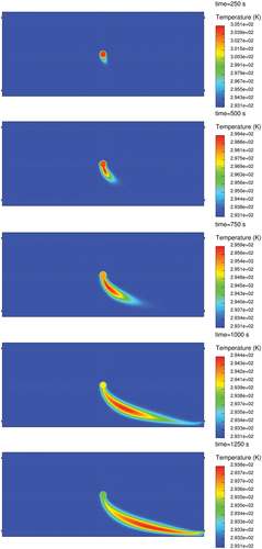
Figure 14 shows the measured temperature at the sensors 8 and 5, varying with the time. Only sensor 8 has a significant temperature development in time, which can be explained by the recirculation flow applied for the experiments (see Figure 12). The water is sucked on the right side near the bottom, and it is injected on the right side at the top. This flow regime leads to a flow in which streamlines develop from the right top corner downwards to the bottom, passing by the heating element, where the water is subject to conductive heat transfer. The glass beads around the heating element are also heated. Therefore, convection and conduction in the ‘porous region’ are superimposed. The energy transport to the outlet at the right bottom corner of the facility is mostly driven by the flow, because the heat conduction through the solid beads is much slower. Figure 15 shows the computed time-dependent temperature development compared to the measured values. It shows simulation results of Star-CCM+ and TinFlow, whereas StarCCM+ does not use a dual-porosity model. The temperature development therefore without the dual-porosity approach is much overestimated. The reason for this is that modelling the porous region only with effective mass averaged properties of fluid plus solid does not represent the local heat storage effect to the structure correctly. Also, the temperature gradient is not predicted in a correct way. Using the dual-porosity approach implemented in TinFlow, the predicted temperature development at sensor position 8 is fitting quite well the measures. This means at the same time that the stored energy in the solid is predicted accurate. Figure 16 shows the fluid temperature distribution at different time points. As it can be seen from this figure, the flow is directed towards the exit at the right bottom side of the test facility. Passing by the heating element the fluid is heated and transfers heat to the solid (in each computational cell there exist a void fraction of fluid and solid which is represented by the porosity and solved by Equations 11(11) $(1-\mathrm{\Phi })(\mathit{\rho }\mathit{c}{)}_s\frac{\mathrm{\partial }{T}_s}{\mathit{dt}}=(1-\mathrm{\Phi })\mathrm{\nabla }\cdot ({\mathit{\lambda }}_s\mathrm{\nabla }{T}_s)+(1-\mathrm{\Phi })q_s^{{ }^{\prime \prime \prime }}+\mathit{h}(T_f-T_s)$(11) and 12(12) $(\mathrm{\Phi })(\mathit{\rho }\mathit{c}{)}_f\frac{\mathrm{\partial }{T}_f}{\mathit{dt}}+(\mathit{\rho }\mathit{c})\vec{v}\cdot \mathrm{\nabla }{T}_f=(\mathrm{\Phi })\mathrm{\nabla }\cdot ({\mathit{\lambda }}_f\mathrm{\nabla }{T}_f)+(\mathrm{\Phi })q_f^{{ }^{\prime \prime \prime }}+\mathit{h}(T_s-T_f)$(12) ). This effect leads to a local heat transfer described by the heat transfer coefficient (see Section 2.2). The decisive measure for local heat transfer and heat storage is $\mathit{h}$ and the storage capacity of the immobile phase of the structure. This measure is crucial for the temperature development over time and for the correct prediction of the heat storage process. A great deal of uncertainty remains. This is the correct calculation of local heat transfer in porous spaces, which differs depending on the type of porosity, the properties of fluid and solid and the flow conditions.

Figure 14. Measured time-dependent temperature for sensor 8 and 5.

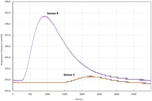
Figure 15. The obtained temperature response at sensor 8. Results of the experiment and simulations with star-CCM+ and TinFlow.

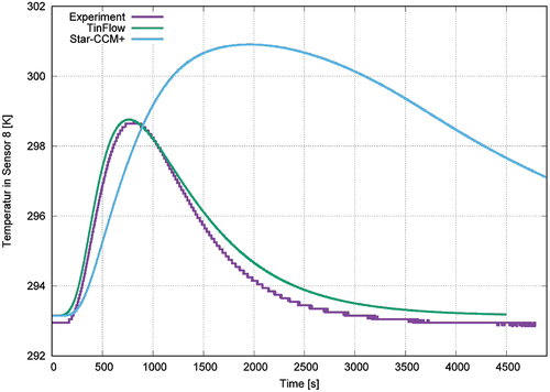
Figure 16. Temperature distribution of a simulation at subsequent time steps in the middle cross-section of the computational domain.

5. Conclusion

In this study, a digital approach was designed that resolves flow dynamics and heat transfer in complex packed beds at millimetre scale. It was used to validate the novel dual-porosity module of the TinFlow solver. In this context, the TinFlow solver was able to predict flow dynamics and heat transfer in a real packed bed that was operated at metre scale. Our approach clearly showed that the dual-porosity approach opens new possibilities for faster computations with good accuracy compared to physically based microstructure resolving the pore space in details. Overall, the methodology presented offers a full digital tool box for solving large-scale heat storage problems in aquifers with a reasonable amount of computer performance and constitutes a decisive step towards both digital and sustainability transformation.

There are important remaining questions in this field, which we will address in the course of the next developments. One important point is related to the anisotropic behaviour of real aquifers. This is mostly unknown, and therefore, a method for numerical experiments with resolved structure (small scale) has to be elaborated to extract the corresponding flow resistance tensors to properly describe the anisotropic permeability of these particular porous media. The second important point is the coupling coefficient $\mathit{h}$, which depends on the local velocity inside a porosity and is not limited by an upper bound. From a physical point of view, this parameter clearly has an upper limit. The determination of limits with a kind of normalization function has been developed, but the maximum permissible value was not yet estimated.

6. Outlook

The dual-porosity method is to be applied to predict the temporal temperature development in a real environment of a water remediation project in Milan. In particular, the flow through dissolved sand grain structures generated and simulated through the simulation framework PACE3D is computed, and the resulting resistance tensors and heat transfer coefficients in the subsoil are extracted for the macroscopic dual-porosity approach. This cross-scale method is applied to achieve numerically the unknowns like the flow resistance tensor and the heat transfer coefficient $\mathit{h}$.

For determining unknown physical properties, active learning with Bayesian optimization, similar to Kulagin et al. (2023) and Zhao et al. (2023), offers a systematic strategy to explore the design space and identify high-performing configurations. In such a strategical framework, Tinflow solvers can be used for accelerated screening, followed by finely-discretized PACE3D simulations only for highly promising configurations. Since the available physical properties only describe the individual porous structure very roughly, significant information loss occurs between resolved and accelerated models. To remedy this information loss, data-driven properties, e.g. through the use of AutoEncoder neural networks (Zhao et al. 2023), can help characterize porous structures with additional low-dimensional parameters.

In addition to the numerical approaches, heat storage experiments were carried out for several days, using a state-of-the-art recirculation system. We hope to show that the prediction of the time dependent heat storage fits quite well with the measured results. The research work will be completed and published in a follow-up forthcoming paper illustrating a milestone in connection with the design of underground heat storage.

Acknowledgments

We thank Federal Ministry of Education and research (BMBF) for funding the project “PoroSan” (FKZ 01IS18013A-C), in which most of these results have emerged. We also thank the Helmholtz Association for supporting the research on porous structure characterization and data interpretations. We acknowledge support by the KIT-Publication Fund of the Karlsruhe Institute of Technology.

Disclosure statement

No potential conflict of interest was reported by the author(s).

Additional information

Funding

The main research has been funded through the BMBF project “PoroSan” [FKZ 01IS18013A-C]. Contributions regarding the porous structure characterization and data interpretations are provided by the support of the Helmholtz Association, programs MSE and KNHFi, no.43.31.01.

References

- Barbe S, Kneer A. 2020. Virtual Material Design: A Powerful Tool for the Development of High-Efficiency Porous Media. In: Membrane Desalination. CRC Press; pp. 269–283.
- Bejan A. 2013. Convection heat transfer. Heboken, New Jersey: John wiley & sons.
- bulletphysics.org. 2022. Bullet real-time physics simulation. Weblink.
- CD-adapco (Ed.), User Guide StarCCM+, Vol. 7.04.006, CD-adapco, 2012.
- Dostál Z, Ladányi L. 2018. Demands on energy storage for renewable power sources. J Energy Storage URL. 18:250–255. https://www.sciencedirect.com/science/article/pii/S2352152X17303857
- Durlofsky L, Brady J. 1987. Analysis of the Brinkman equation as a model for flow in porous media. Phys Fluids. 30(11):3329–3341. doi: 10.1063/1.866465.
- Ferziger J, Peric M. 1997. Computational methods for fluid dynamics. Heidelberg: Springer.
- Hernandez A. 2005. Combined Flow and Heat Transfer Characterization of open cell Aluminium Foams, Master Thesis, University of Puerto Rico.
- Hötzer J, Reiter A, Hierl H, Steinmetz P, Selzer M, Nestler B. 2018. The parallel multi-physics phase-field framework PACE3D. J Comput Sci. 26:1–12. doi: 10.1016/j.jocs.2018.02.011.
- Jarullah A, Noor A. 2019. Energy consumption and heat recovery of an industrial fluidized catalytic cracking process based on cost savings. Appl Petrochem Res. 9(1):1–11. doi: 10.1007/s13203-018-0217-6.
- Kneer A, Ed. 2022. User guide TinFlow, vol. V2.402. TinniT Technologies GmbH.
- Kopanadis AGE, Theodorakakos BD, Gavaises E, Bouris D. 2010. 3D numerical simulation of flow and conjugate heat transfer through a pore scale model of high porosity open cell metal foam. International Journal Of Heat And Mass Transfer. 53(11–12):2539–2550. doi: 10.1016/j.ijheatmasstransfer.2009.12.067.
- Kulagin R, Reiser P, Truskovskyi K, Koeppe A, Beygelzimer Y, Estrin Y, Friederich P, Gumbsch P. 2023. Lattice metamaterials with mesoscale motifs: exploration of property charts by Bayesian optimization. Adv Eng Mater. 25(13):2300048. doi: 10.1002/adem.202300048.
- Kunii D, Suzuki M. 1967. Particle-to-fluid heat and mass transfer in packed beds of fine particles. Int J Heat Mass Transfer. 10(1967):845–852. Pergamon Press Ltd. doi: 10.1016/0017-9310(67)90064-6.
- Laurien JH, und Oertel E. 2003. Numerische Strömungsmechanik, Vol. 8. überarbeitete Auflage, Viehweg Verlag, Fried. Braunschweig/Wiesbaden: Vieweg und Sohn Verlagsgesellschaft mbH.
- Nield D, Bejan A. 2013. Convection in porous media. 4th ed. New York Heidelberg Dordrecht London: Springer.
- Peszynska A, Trykozko M, Sobieski W. 2010. Forchheimer law in computational and experimental studies of flow through porous media at porescale and mesoscale. GAKUTO International Series, Mathematical Sciences And Applications. 32:463–482.
- Pierro L, Matturro B, Rossetti S, Sagliaschi M, Sucato S, Alesi E, Bartsch E, Arjmand F, Petrangeli PM. 2017. Polyhydroxyalkanoate as a slow-release carbon source for in situ bioremediation of contaminated aquifers: from laboratory investigation to pilot-scale testing in the field. New Biotechnol. 37:60–68. doi: 10.1016/jnbt.2016.11.004.
- Prajapati N, Hermann C, Späth M, Schneider D, Selzer M, Nestler B. 2020. Brittle anisotropic fracture propagation in Quartz Sandstone: insights from phase-field simulations. Comput Geosci. 24(3):1361–1376. doi: 10.1007/s10596-020-09956-3.
- Prajapati N, Selzer M, Nestler B, Busch B, Hilgers C, Ankit K. 2018. Three-dimensional phase- field investigation of pore space cementation and permeability in Quartz Sandstone. JGR Solid Earth. 123(8):6378–6396. doi: 10.1029/2018JB015618.
- Quintard M, Whitaker S. 1994a. Convection, Dispersion, and interfacial Transport of Contaminants: Homogeneous porous Media. Adv Water Resour. 17(4):221–239. doi: 10.1016/0309-1708(94)90002-7.
- Quintard M, Whitaker S. 1994b. Transport in ordered and disordered porous media IV: computer generated porous media for three-dimensional systems. Transp Porous Media. 15(1):51–70. doi: 10.1007/BF01046158.
- Quintard M, Whitaker S. 1997a. Transport in chemically and mechanically heterogeneous porous media - IV, large-scale mass equilibrium for solute transport with adsorption. Adv Water Resour. 22(1):33–57. doi: 10.1016/S0309-1708(97)00027-4.
- Quintard M, Whitaker S. 1997b. Transport in chemically and mechanically heterogeneous porous media—III. Large-scale mechanical equilibrium and the regional form of Darcy’s law. Adv Water Resour. 21(7):617–629. doi: 10.1016/S0309-1708(97)00015-8.
- Qu Z, Xu H, Wang T, Tao W, Lu T. 2013. Thermal transport in metallic porous media, key laboratory of thermal fluid science and engineering, key laboratory of strength and vibration. China www.intechopen.com:UniversityinXi’an.
- Schlichting H, Gersten K. 2003. Grenzschichttheorie. Berlin Heidelberg: Springer-Verlag.
- Shi Z, Wang X, Comparison of Darcy’s law, the Brinkman equation, the modified N-S equation and the pure diffusion equation in PEM fuel cell modeling, in: Comsol conference, Boston, 2007.
- Simons S, Schmitt J, Tom B, Bao H, Pettinato B, Pechulis M. 2021. Chapter 10 - advanced concepts. in Brun K, Allison T Dennis R. editors. Thermal, mechanical, and hybrid chemical energy storage systems. Academic Press. pp. 569–596. doi: 10.1016/B978-0-12-819892-6.00010-1
- Sommer W, Drijver B, Verburg R, Slenders H, De Vries E, Dinkla I, Leusbrock I, Grotenhuis T. 2013. Combining shallow geothermal energy and groundwater remediation. European Geothermal Congress. https://library.wur.nl/WebQuery/wurpubs/fulltext/264023.
- Srinivasan S, Nakshatrala K. 2010. A stabilizes mixed formulation for unsteady Brinkman equation based on the method of horizontal lines, cs.NA. Int J Numer Methods Fluids. 68(5):642–670. doi: 10.1002/fld.2544.
- Summ G, Lösbarkeit und Dikretisierung der gemischten Formulierung für Darcy-Forchheimer- Fluss in porösen Medien, Ph.D. thesis, Friedrich-Alexander-Universität Erlangen-Nürnberg, Naturwissenschaftliche Fakultäten (2001).
- Taylor GI. 1954.“Conditions under which dispersion of a solute in a stream of solvent can be used to measure molecular diffusion.” Proceedings of the Royal Society of London. Series A. Mathematical and Physical Sciences 225.1163; pp. 473–477.
- Toride FVGM, Leij N, The CXTFIT code for estimating transport parameters from laboratory or field tracer experiments version 2.1, Tech. rep. (1999).
- Vafai K, Tien C. 1981. Boundary and inertia effects on flow and heat transfer in porous media. J Heat Transfer. 24(2):195–203. doi: 10.1016/0017-9310(81)90027-2.
- van Genuchten M, Wagenet R. 1989. Two-site-two-region models for pesticide transport and degradation: theoretical development and analytical solutions. Vol. 53. Amsterdam: Soil Science Society; pp. 1303–1310.
- Vdi VGVUCG. 2006. Verein Deutscher Ingenieure, VDI-Wärmeatlas. 10th ed. Berlin, Heidelberg, New-York: Springer.
- Whitaker S. 1967. Diffusion and dispersion in porous media, A.I.Ch.E. AichE J. 13(3):420–427. doi: 10.1002/aic.690130308.
- Whitaker S. 1986a. Flow in porous media I: a theoretical derivation of Darcy’s law. Transp Porous Media. 1(1):3–25. doi: 10.1007/BF01036523.
- Whitaker S. 1986b. Flow in porous media II: the governing equations for immiscible, two-phase flow, transport in porous media. Transp Porous Media. 1(2):105–125. doi: 10.1007/BF00714688.
- Whitaker S. 1996. The Forchheimer equation: a theoretical development. Transp Porous Media. 25(1):27–61. doi: 10.1007/BF00141261.
- Xu J, Li Y, Wang R, Liu W. 2014. Performance investigation of a solar heating system with underground seasonal energy storage for greenhouse application. Energy. 67:63–73. doi: 10.1016/j.energy.2014.01.049
- Yang K, Vafai K. 2011. Transient aspects of heat flux bifurcation in porous media: an exact solution. J Heat Transfer. 133(52602):1–12. doi: 10.1115/1.4003047.
- Zhao Y, Altschuh P, Santoki J, Griem L, Tosato G, Selzer M, Koeppe A, Nestler B. 2023. Characterization of porous membranes using artificial neural networks. Acta Mater. 253:118922. doi: 10.1016/j.actamat.2023.118922.
- Zhu ZH, Wen Q, Zhan H, Yuan S. 2020. Optimization strategies for in situ groundwater remediation by a vertical circulation well based on particle-tracking and node dependent finite difference methods. Water Resour. 56(11): doi: 10.1029/2020WR027396.
- Zierep J, Bühler K. 2010. Grundzüge der Strömungslehre. In: überarbeitete Auflage, Viehweg +. Teubner Verlag, Springer Fachmedien Wiesbaden GmbH; pVol. 8.