Fractional dynamics and sensitivity analysis of measles epidemic model through vaccination

Abstract

Measles is a highly contagious disease that mainly affects children worldwide. Even though a reliable and effective vaccination is available, there were 140,000 measles deaths worldwide in 2018, and most of them were children under the age five years. In this paper, we comprehensively investigate a novel fractional SVEIR (Susceptible-Vaccinated-Exposed-Infected-Recovered) model of the measles epidemic powered by nonlinear fractional differential equations to understand the epidemic’s dynamical behaviour. We use a non-singular Atangana-Baleanu fractional derivative to analyze the proposed model, taking advantage of non-locality. The existence, uniqueness, positivity and boundedness of the solutions are shown via concepts of fixed point theory, and we also perform the Ulam-Hyers stability of the considered model. The parameter sensitivity is discussed in the context of the variance with each parameter using 3-D graphics based on the basic reproduction number. Moreover, with the Atangana-Toufik numerical scheme, numerical findings are depicted for different fractional-order values. The presented approach produce results that are efficiently consistent and in excellent agreement with the theoretical results.

Keywords:

• Atangana-Baleanu derivative
• measles
• numerical analysis
• sensitivity analysis
• Ulam-Hyers stability

1. Introduction

Measles is also named as morbilli or rubeola, is an infectious disease resulted by the Morbillivirus, a species of the Paramyxoviridae family. It specifically targets children under five and has a significant fatality rate. The measles virus is vaccine-preventable, yet the World Health Organization (WHO) still considers this disease to be a public health issue (Budigan Ni et al., 2023; Center of Disease Control and Prevention, n.d; Gambrell, Sundaram, & Bednarczyk, 2022). Disease reported the lives of over 110,000 persons in 2017 especially young children (James Peter, Ojo, Viriyapong, & Abiodun Oguntolu, 2022). Table 1 presents the ten states that the disease outbreak has most profoundly influenced. The number of confirmed cases of measles in 2019 was, interestingly, the most in the previous two decades. Meantime, measles outbreaks have been highlighted in 2019 in many nations, including Angola, Cameroon, Sudan, Nigeria, Chad, Congo, Madagascar, and South Sudan in Africa, Kazakhstan in Central Asia, the Philippines and Thailand in Southeast Asia, and Ukraine in Eastern Europe (Callister, 2019). In 182 countries, there were 364,811 cases reported in the first quarter of 2019, as stated in the WHO statistics. Moreover, massive increase in measles cases were seen in the Western Pacific, European and African zones (Jost, Luzi, Metzler, Miran, & Mutsch, 2015).

Table 1. List of top five nations with worldwide measles outbreaks (7)(7) $$\mathcal{L}{\{}^{\mathit{\text{ABC}}}{D}_0^{\vartheta }\mathbf{U}(t)\}(s)=[\frac{s^{\vartheta }\mathcal{L}\{\mathbf{U}(t)\}(s)-s^{\vartheta -1}\mathbf{U}(0)}{s^{\vartheta }(1-\vartheta )+\vartheta }]\times \mathcal{M}(\vartheta ).$$(7) .

Country	Rank	Number of cases
India	1	12,271
Yemen	2	7,538
Somalia	3	6,261
Zimbabwe	4	4,623
Pakistan	5	2,586

The first flu-like measles symptoms occur 7 to 14 days after the first virus contacts the human host. Within two to five days of the initial symptoms, skin rashes and Koplik spots within the mouth of the influenced person happen, and the rashes then diffuse to the rest of the body. This viral infection spreads with the signs of high fever, rash development, cough, a runny nose, red and watery eyes. Approximately one-third of all diagnosed cases are expected to have significant consequences, such as pneumonia, acute encephalitis, and common problems like diarrhoea and skin infections (Battegay, Itin, & Itin, 2012; Gould, 2015). Furthermore, respiratory droplets caused by sneezing and coughing, direct communication with contaminated noses or throat secretions and close physical contact spread the measles virus from person to person (Angelo et al., 2019). Policies corresponding to vaccination play an essential role in preventing the human host from disease. Many vaccinations have been made to protect hosts from widespread infections in certain areas (Ilesanmi, Adeyinka, & Olakunde, 2022; Vojtek, Larson, Plotkin, & Van Damme, 2022). It is accurate to say that some of these vaccinations are expensive, some have adverse effects, and none are entirely adequate. It is also claimed that the development of a low-cost, beneficial, and safe vaccine, coupled with faster immunization programs has led to an 80% reduction in measles-related moralities, particularly in industrialized nations (Fisker et al., 2022).

To develop practical mitigation actions to eliminate and prevent measles, policymakers conducted a wide range of studies. Quantitative methodologies are required to assess the cost-effectiveness and effect of these activities in order to enhance them in the future (Ain & Wang, 2023; Pokharel, Adhikari, Gautam, Uprety, & Vaidya, 2022). Mathematical modelling has greatly aided in visualizing, studying, and comprehending the transmission mechanism of several diseases (Khan & Atangana, 2022; Raza, Arshed, Bakar, Shahzad, & Inc, 2023). Moreover, these models enable efficient control policies for the determent of future infection. The mathematical analysis of these models provides vital findings of infection and estimates future consequences that are hard to quantify under other conditions (Abbasi, Zamani, Mehra, Shafieirad, & Ibeas, 2020; Khan, Ullah, Ali, & Zaman, 2019; Tyagi, Gupta, Abbas, Das, & Riadh, 2021). Furthermore, for some recent and interesting results related to nonlinear fractional boundary value problems, fractional integro-differential equations, tuberculosis model using different fractional derivatives, etc. see (Batool, Talib, Riaz & Tunç, 2022; Bohner, Tunç & Tunç, 2021; Graef, Tunç & Şevli 2021; Tunç, Tunç &Yao, 2021; Tunç & Tunç, 2023; Zafar, Zaib, Hussain, Tunç & Javeed, 2022). Numerous epidemic models have been constructed to better explain the biological mechanism of measles disease outbreak (Ochoche & Gweryina, 2014; Sowole, Ibrahim, Sangare, & Lukman, 2020). It is also used to analyze the effectiveness of health care initiatives and indicate the ideal plan of action for fighting measles, including how to utilize the vaccination efficiently. The literature (Liu, Ikram, Khan, & Din, 2022; Memon, Qureshi, & Memon, 2020) uses various measles models for real-world data to forecast disease transmission and control.

The fact that fractional order models (FOMs) provide more proficient, in-depth, reliable, and valuable information concerning the dynamics of many diseases than traditional models is evident. Its hereditary features and memory characterization make it special to traditional models (Ain, Khan, Abdeljawad, Gómez-Aguilar, & Riaz, 2024; Ain et al., 2022; Alzahrani & Khan, 2020; Baishya, Achar, Veeresha, & Prakasha, 2021; Raza, Bakar, Khan, & Tunç, 2022; Singh, Kumar, Hammouch, & Atangana, 2018; Tao, Anjum, & Yang, 2023). FOMs make it easier to investigate and illustrate the dynamics between two non-local locations. Several concepts and theories have been presented and established regarding fractional order derivatives (Uchaikin, 2013; Yang, 2019). In Ref. (Samko, Kilbas, & Marichev, 1993) the essential concept and principle of the fractional calculus are presented. Fractional derivatives have been proven to be an excellent tool for simulating real-world issues in various fields, including engineering, physics, economics, and biology. FOMs offer more reliable, accurate, and consistent insights into the dynamics of disease resulting from a biological system (Anjum, Ain, & Li, 2021; Anjum, He, & He, 2021; Butt, Ahmad, Rafiq, & Baleanu, 2022; Conlan, Rohani, Lloyd, Keeling, & Grenfell, 2010; Farman, Saleem, Ahmad, & Ahmad, 2018; Qureshi & Jan, 2021). The researchers in Ref. (Butt, Ahmad Saqib, Alshomrani, Bakar, & Inc, 2024) discuss the dynamic characteristics of the fractional cervical cancer system, along with the sensitivity of the basic reproduction number. To compare the outcomes of the suggested model with the integer-order model, Abboubakkar et al. Abboubakar, Fandio, Sofack, and Ekobena Fouda, (2022) designed a mathematical model for measles employing the Caputo derivative. The study in Ref. (Nabti & Ghanbari, 2021) examines an SVEIR measles fractional framework, demonstrating the existence and uniqueness of the measles fractional model while dividing the population into five subcategories. Ahmad et al. (2024) have utilized vaccination impact as a control strategy for the dynamics of COVID-19. In their work to prevent Hepatitis disease, Ain and Chu (2004) studied the impact of vaccines in the Hepatitis model.

In this study, we employ a fractional system to elucidate the dynamics of measles transmission in the presence of vaccination, serving as the conceptual foundation for the preceding discussion. We also evaluated and assessed the effect of different parameters of this model on the results of the basic reproduction number in order to identify the most important aspects of disease control and prevention. Also noteworthy is that the measles model presented here is a newly developed model that has been examined for the first time in the context of the current research using the ABC fractional operator. Moreover, some new research studies either overlook the significance of sensitivity analysis of ${\mathcal{R}}_0^M$ or do so by analyzing local forward sensitivity indices to figure out the critical epidemiological model parameters that affect ${\mathcal{R}}_0^M.$ For the numerical solution, we use the Atangana-Toufik method (ATM) from the literature (Toufik & Atangana, 2017).

The remaining article is further structured into the following sections: Section 2 presented some fundamental results after developing a dynamical system for measles spread within the environment of both traditional and fractional derivatives. In Section 3, we investigated the suggested model for the qualitative analysis, including the existence, uniqueness, and positivity of the solution for the proposed model. The dynamical aspect of the presented model, such as stability analysis, and the fundamental reproduction number ${\mathcal{R}}_0^M$ is examined and computed. In Section 4, a sensitivity analysis of ${\mathcal{R}}_0^M$ is performed. To understand the dynamics of the suggested model with the ABC derivative operator, a numerical approach with illustrations is introduced in Section 5. Section 6 summarizes the stated research work and offers future prospects.

2. Measles model with the ABC derivative

We consider a mathematical model with five categories for the spread of measles disease in a particular region based primarily on individuals status. Following are the epidemiological classes into which the compartments are classified. Susceptible humans $\mathbb{S}(t)$ who are at risk or susceptible to acquiring measles, vaccinated humans $\mathbb{V}(t)$ who have received a measles vaccination, exposed humans $\mathbb{E}(t)$ who have been revealed symptoms of measles, infected humans $\mathbb{I}(t)$ who have measles and are transmittable, and recovered humans $\mathbb{R}(t)$ who have measles and have been naturally healed. For those in this class, the body’s immunity becomes permanently resilient to the ailment after the cure, preventing further infection and recurrence. It is also assumed that there is no infection after the recovery and the total population will remain constant at any time. Figure 1 provide a pictorial illustration of the model.

Figure 1. Schematic illustration of the measles transmission in the population.

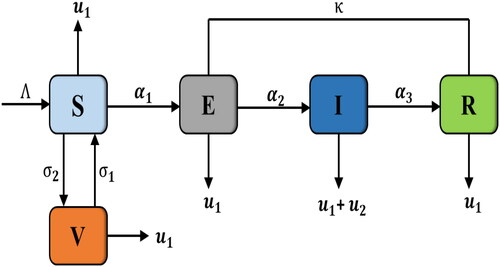
Therefore, the following system describes the dynamics of measles transmission in the human population can be expressed as: (1) $$\{\begin{array}{ccc}\stackrel{.}{\mathbb{S}}(t)\hfill & =\hfill & \Lambda -{\alpha }_1\mathbb{S}\mathbb{I}+{\sigma }_1\mathbb{V}-({\mu }_1+{\sigma }_2)\mathbb{S},\hfill \\ \stackrel{.}{\mathbb{V}}(t)\hfill & =\hfill & {\sigma }_2\mathbb{S}-({\mu }_1+{\sigma }_1)\mathbb{V},\hfill \\ \stackrel{.}{\mathbb{E}}(t)\hfill & =\hfill & {\alpha }_1\mathbb{S}\mathbb{I}-({\alpha }_2+\kappa +{\mu }_1)\mathbb{E},\hfill \\ \stackrel{.}{\mathbb{I}}(t)\hfill & =\hfill & {\alpha }_2\mathbb{E}-({\mu }_2+{\alpha }_3+{\mu }_1)\mathbb{I},\hfill \\ \stackrel{.}{\mathbb{R}}(t)\hfill & =\hfill & \kappa \mathbb{E}+{\alpha }_3\mathbb{I}-{\mu }_1\mathbb{R}.\hfill \end{array}$$(1)

The system described in (1)(1) $$\{\begin{array}{ccc}\stackrel{.}{\mathbb{S}}(t)\hfill & =\hfill & \Lambda -{\alpha }_1\mathbb{S}\mathbb{I}+{\sigma }_1\mathbb{V}-({\mu }_1+{\sigma }_2)\mathbb{S},\hfill \\ \stackrel{.}{\mathbb{V}}(t)\hfill & =\hfill & {\sigma }_2\mathbb{S}-({\mu }_1+{\sigma }_1)\mathbb{V},\hfill \\ \stackrel{.}{\mathbb{E}}(t)\hfill & =\hfill & {\alpha }_1\mathbb{S}\mathbb{I}-({\alpha }_2+\kappa +{\mu }_1)\mathbb{E},\hfill \\ \stackrel{.}{\mathbb{I}}(t)\hfill & =\hfill & {\alpha }_2\mathbb{E}-({\mu }_2+{\alpha }_3+{\mu }_1)\mathbb{I},\hfill \\ \stackrel{.}{\mathbb{R}}(t)\hfill & =\hfill & \kappa \mathbb{E}+{\alpha }_3\mathbb{I}-{\mu }_1\mathbb{R}.\hfill \end{array}$$(1) has already been studied in Ref. (Peter, Qureshi, Ojo, Viriyapong, & Soomro, 2022). Besides that, this model does not account for the memory effects, which are found in several biological models. To expedite the reduction of measles prevalence, this methodology aims to enhance both diagnosis and therapy for individuals exposed to the disease. Therefore, we modify the framework by replacing the traditional derivative with the recently proposed ABC fractional derivative, permitting the model to account for memory characteristics. Let us first construct the fractional illustration of the considered system by using the ABC operator: (2) $$\{\begin{array}{ccc}{}_0^{\mathit{\text{ABC}}}{D}_t^{\vartheta }\mathbb{S}(t)\hfill & =\hfill & \Lambda -{\alpha }_1\mathbb{S}\mathbb{I}+{\sigma }_1\mathbb{V}-({\mu }_1+{\sigma }_2)\mathbb{S},\hfill \\ {}_0^{\mathit{\text{ABC}}}{D}_t^{\vartheta }\mathbb{V}(t)\hfill & =\hfill & {\sigma }_2\mathbb{S}-({\mu }_1+{\sigma }_1)\mathbb{V},\hfill \\ {}_0^{\mathit{\text{ABC}}}{D}_t^{\vartheta }\mathbb{E}(t)\hfill & =\hfill & {\alpha }_1\mathbb{S}\mathbb{I}-({\alpha }_2+\kappa +{\mu }_1)\mathbb{E},\hfill \\ {}_0^{\mathit{\text{ABC}}}{D}_t^{\vartheta }\mathbb{I}(t)\hfill & =\hfill & {\alpha }_2\mathbb{E}-({\mu }_2+{\alpha }_3+{\mu }_1)\mathbb{I},\hfill \\ {}_0^{\mathit{\text{ABC}}}{D}_t^{\vartheta }\mathbb{R}(t)\hfill & =\hfill & \kappa \mathbb{E}+{\alpha }_3\mathbb{I}-{\mu }_1\mathbb{R},\hfill \end{array}$$(2) with the following initial constraints $$\mathbb{S}(0)\ge 0,\mathbb{V}(0)\ge 0,\mathbb{E}(0)\ge 0,\mathbb{I}(0)\ge 0,\mathbb{R}(0)\ge 0,$$ where $0<t<T$ and ${}_0^{\mathit{\text{ABC}}}{D}_t^{\vartheta }$ signifies the ABC derivative of order $\vartheta \in (0,1).$

2.1. Fundamental results

In this section of the study, we will present some fundamental concepts that will be useful for our computations in the remaining sections.

Definition 1.

The following expression (Butt et al., 2024) defines the fractional derivative of Riemann-Liouville with order $\vartheta$ and $n-1<\vartheta \le n$ as: (3) $${}^{\mathit{\text{RL}}}{D}_0^{\vartheta }\mathbf{U}(t)=\frac{1}{\Gamma (n-\vartheta )}\frac{d^n}{d{t}^n}{\int }_0^t\mathbf{U}(\omega ){(t-\omega )}^{n-\vartheta -1}d\omega .$$(3)

Definition 2.

The Caputo fractional derivative of order $\vartheta$ and $n-1<\vartheta \le n$ is stated in the following way (Butt et al., 2024): (4) $${}^C{D}_0^{\vartheta }\mathbf{U}(t)=\frac{1}{\Gamma (n-\vartheta )}{\int }_0^t{(t-\omega )}^{n-\vartheta -1}\frac{d^n}{d{t}^n}\mathbf{U}(\omega )d\omega .$$(4)

Definition 3.

(Butt et al., 2022) A mapping $\mathbf{U}(t)$ with the constraint that $\mathbf{U}(t)\in H^1[0,T],$ then the ABC derivative of order $\vartheta \in [0,1]$ is defined as following: (5) $${}_a^{\mathit{\text{ABC}}}{D}_t^{\vartheta }\mathbf{U}(t)=\frac{\mathcal{M}(\vartheta )}{1-\vartheta }{\int }_a^t\dot{\mathbf{U}}(\omega )E_{\vartheta }[-\vartheta \frac{{(t-\omega )}^{\vartheta }}{1-\vartheta }]d\omega ,$$(5) where $\mathcal{M}(\vartheta ),$ is a normalization constant with the property that $\mathcal{M}(0)=1=\mathcal{M}(1),$ and $E_{\vartheta }$ is a ML operator, and defined by $$E_{\vartheta }(\xi )=\sum _{k=0}^{\infty }\frac{{\xi }^k}{\Gamma (k\vartheta +1)}.$$

Definition 4.

(Din, Li, Khan, Khan, & Liu, 2022) The non-integer integration of a mapping $\mathbf{U}(t),$ taking $0<\mathbf{U}\le T$ in the sense of ABC derivative is defined as: (6) $${}^{\mathit{\text{ABC}}}{I}_{+0}^{\vartheta }\mathbf{U}(t)=\frac{1-\vartheta }{\mathcal{M}(\vartheta )}\mathbf{U}(t)+\frac{\vartheta }{\mathcal{M}(\vartheta )\Gamma (\vartheta )}{\int }_0^t\mathbf{U}(\omega ){(t-\omega )}^{\vartheta -1}d\omega .$$(6)

Definition 5.

(Butt et al., 2022) The Laplace transform (LT) in the ABC sense for a mapping $\mathbf{U}(t)$ can be stated as: (7) $$\mathcal{L}{\{}^{\mathit{\text{ABC}}}{D}_0^{\vartheta }\mathbf{U}(t)\}(s)=[\frac{s^{\vartheta }\mathcal{L}\{\mathbf{U}(t)\}(s)-s^{\vartheta -1}\mathbf{U}(0)}{s^{\vartheta }(1-\vartheta )+\vartheta }]\times \mathcal{M}(\vartheta ).$$(7)

Theorem 1.

(Din et al., 2022) The following fractional order problem(8) $$\begin{array}{c}\{\begin{array}{c}{}^{\mathit{\text{ABC}}}{D}_{+0}^{\vartheta }\mathbf{U}(t)=\Phi (t,\mathbf{U}(t)),\text{for all} t\in [0,T],\hfill \\ \mathbf{U}(0)={\mathbf{U}}_0,\hfill \end{array}\hfill \end{array}$$(8) has a unique solution(9) $$\mathbf{U}(t)=\mathbf{U}(0)+\frac{1-\vartheta }{\mathcal{M}(\vartheta )}\mathbf{U}(t)+\frac{\vartheta }{\mathcal{M}(\vartheta )\Gamma (\vartheta )}{\int }_0^t\mathbf{U}(\omega ){(t-\omega )}^{\vartheta -1}d\omega .$$(9)

Theorem 2.

(Zafar et al., 2022) Consider a convex subset $\mathbf{U}$ of ${\Omega }_{\beta }$ and also assume that ${\Psi }_1,{\Psi }_2$ with

1. ${\Psi }_1\mathbf{U}+{\Psi }_2\mathbf{U}\in {\Omega }_{\beta },\text{for all} \mathbf{U}\in {\Omega }_{\beta },$

2. ${\Psi }_1$ is contraction,

3. ${\Psi }_2$ is a continuous and compact set,

with the operator equation ${\Psi }_1\mathbf{U}+{\Psi }_2\mathbf{U}=\mathbf{U}$, has one or more solutions.

3. Qualitative analysis

In this part, we employed Banach fixed point theorems to establish the existence and uniqueness of the given system, in addition to the Ulam-Hyers stability of the analyzed model under the ABC derivative. Also, we compute the equilibrium states and fundamental reproduction number for the suggested system.

3.1. Existence and uniqueness of solutions for the measles model

In order to examine the existence of the solution of the non-integer model (2)(2) $$\{\begin{array}{ccc}{}_0^{\mathit{\text{ABC}}}{D}_t^{\vartheta }\mathbb{S}(t)\hfill & =\hfill & \Lambda -{\alpha }_1\mathbb{S}\mathbb{I}+{\sigma }_1\mathbb{V}-({\mu }_1+{\sigma }_2)\mathbb{S},\hfill \\ {}_0^{\mathit{\text{ABC}}}{D}_t^{\vartheta }\mathbb{V}(t)\hfill & =\hfill & {\sigma }_2\mathbb{S}-({\mu }_1+{\sigma }_1)\mathbb{V},\hfill \\ {}_0^{\mathit{\text{ABC}}}{D}_t^{\vartheta }\mathbb{E}(t)\hfill & =\hfill & {\alpha }_1\mathbb{S}\mathbb{I}-({\alpha }_2+\kappa +{\mu }_1)\mathbb{E},\hfill \\ {}_0^{\mathit{\text{ABC}}}{D}_t^{\vartheta }\mathbb{I}(t)\hfill & =\hfill & {\alpha }_2\mathbb{E}-({\mu }_2+{\alpha }_3+{\mu }_1)\mathbb{I},\hfill \\ {}_0^{\mathit{\text{ABC}}}{D}_t^{\vartheta }\mathbb{R}(t)\hfill & =\hfill & \kappa \mathbb{E}+{\alpha }_3\mathbb{I}-{\mu }_1\mathbb{R},\hfill \end{array}$$(2) , let us consider the model in the below form: (10) $$\{\begin{array}{ccc}{}_0^{\mathit{\text{ABC}}}{D}_t^{\vartheta }\mathbb{S}(t)\hfill & =\hfill & {\mathbb{G}}_1(t,\mathbb{S},\mathbb{V},\mathbb{E},\mathbb{I},\mathbb{R}),\hfill \\ {}_0^{\mathit{\text{ABC}}}{D}_t^{\vartheta }\mathbb{V}(t)\hfill & =\hfill & {\mathbb{G}}_2(t,\mathbb{S},\mathbb{V},\mathbb{E},\mathbb{I},\mathbb{R}),\hfill \\ {}_0^{\mathit{\text{ABC}}}{D}_t^{\vartheta }\mathbb{E}(t)\hfill & =\hfill & {\mathbb{G}}_3(t,\mathbb{S},\mathbb{V},\mathbb{E},\mathbb{I},\mathbb{R}),\hfill \\ {}_0^{\mathit{\text{ABC}}}{D}_t^{\vartheta }\mathbb{I}(t)\hfill & =\hfill & {\mathbb{G}}_4(t,\mathbb{S},\mathbb{V},\mathbb{E},\mathbb{I},\mathbb{R}),\hfill \\ {}_0^{\mathit{\text{ABC}}}{D}_t^{\vartheta }\mathbb{R}(t)\hfill & =\hfill & {\mathbb{G}}_5(t,\mathbb{S},\mathbb{V},\mathbb{E},\mathbb{I},\mathbb{R}),\hfill \end{array}$$(10) where (11) $$\{\begin{array}{ccc}{\mathbb{G}}_1(t,\mathbb{S},\mathbb{V},\mathbb{E},\mathbb{I},\mathbb{R})\hfill & =\hfill & \Lambda -{\alpha }_1\mathbb{S}\mathbb{I}+{\sigma }_1\mathbb{V}-({\mu }_1+{\sigma }_2)\mathbb{S},\hfill \\ {\mathbb{G}}_2(t,\mathbb{S},\mathbb{V},\mathbb{E},\mathbb{I},\mathbb{R})\hfill & =\hfill & {\sigma }_2\mathbb{S}-({\mu }_1+{\sigma }_1)\mathbb{V},\hfill \\ {\mathbb{G}}_3(t,\mathbb{S},\mathbb{V},\mathbb{E},\mathbb{I},\mathbb{R})\hfill & =\hfill & {\alpha }_1\mathbb{S}\mathbb{I}-({\alpha }_2+\kappa +{\mu }_1)\mathbb{E},\hfill \\ {\mathbb{G}}_4(t,\mathbb{S},\mathbb{V},\mathbb{E},\mathbb{I},\mathbb{R})\hfill & =\hfill & {\alpha }_2\mathbb{E}-({\mu }_2+{\alpha }_3+{\mu }_1)\mathbb{I},\hfill \\ {\mathbb{G}}_5(t,\mathbb{S},\mathbb{V},\mathbb{E},\mathbb{I},\mathbb{R})\hfill & =\hfill & \kappa \mathbb{E}+{\alpha }_3\mathbb{I}-{\mu }_1\mathbb{R}.\hfill \end{array}$$(11)

The following model will be used for the communication of (2)(2) $$\{\begin{array}{ccc}{}_0^{\mathit{\text{ABC}}}{D}_t^{\vartheta }\mathbb{S}(t)\hfill & =\hfill & \Lambda -{\alpha }_1\mathbb{S}\mathbb{I}+{\sigma }_1\mathbb{V}-({\mu }_1+{\sigma }_2)\mathbb{S},\hfill \\ {}_0^{\mathit{\text{ABC}}}{D}_t^{\vartheta }\mathbb{V}(t)\hfill & =\hfill & {\sigma }_2\mathbb{S}-({\mu }_1+{\sigma }_1)\mathbb{V},\hfill \\ {}_0^{\mathit{\text{ABC}}}{D}_t^{\vartheta }\mathbb{E}(t)\hfill & =\hfill & {\alpha }_1\mathbb{S}\mathbb{I}-({\alpha }_2+\kappa +{\mu }_1)\mathbb{E},\hfill \\ {}_0^{\mathit{\text{ABC}}}{D}_t^{\vartheta }\mathbb{I}(t)\hfill & =\hfill & {\alpha }_2\mathbb{E}-({\mu }_2+{\alpha }_3+{\mu }_1)\mathbb{I},\hfill \\ {}_0^{\mathit{\text{ABC}}}{D}_t^{\vartheta }\mathbb{R}(t)\hfill & =\hfill & \kappa \mathbb{E}+{\alpha }_3\mathbb{I}-{\mu }_1\mathbb{R},\hfill \end{array}$$(2) as: (12) $$\begin{array}{c}\{\begin{array}{c}{}_0^{\mathit{\text{ABC}}}{D}_t^{\vartheta }\mathbf{Z}(t)=\Phi (t,\mathbf{Z}(t)),\hfill \\ \mathbf{Z}(0)={\mathbf{Z}}_0.\hfill \end{array}\hfill \end{array}$$(12)

Using Equation (5)(5) $${}_a^{\mathit{\text{ABC}}}{D}_t^{\vartheta }\mathbf{U}(t)=\frac{\mathcal{M}(\vartheta )}{1-\vartheta }{\int }_a^t\dot{\mathbf{U}}(\omega )E_{\vartheta }[-\vartheta \frac{{(t-\omega )}^{\vartheta }}{1-\vartheta }]d\omega ,$$(5) , the above system becomes (13) $$\mathbf{Z}(t)={\mathbf{Z}}_0(t)+\{\Phi (t,\mathbf{Z}(t))-{\Phi }_0(t)\}\frac{1-\vartheta }{\mathcal{M}(\vartheta )}+\frac{\vartheta }{\mathcal{M}(\vartheta )\Gamma (\vartheta )}{\int }_0^t\Phi (\rho ,\mathbf{Z}(\rho )){(t-\rho )}^{\vartheta -1}d\rho ,$$(13) where (14) $$\begin{array}{c}\mathbf{Z}(t)=\{\begin{array}{c}\mathbb{S}(t)\hfill \\ \mathbb{V}(t)\hfill \\ \mathbb{E}(t)\hfill \\ \mathbb{I}(t)\hfill \\ \mathbb{R}(t)\hfill \end{array},\mathrm{\hspace{1em}}\mathrm{\hspace{1em}}{\mathbf{Z}}_0(t)=\{\begin{array}{c}{\mathbb{S}}_0(t)\hfill \\ {\mathbb{V}}_0(t)\hfill \\ {\mathbb{E}}_0(t)\hfill \\ {\mathbb{I}}_0(t)\hfill \\ {\mathbb{R}}_0(t)\hfill \end{array},\hfill \end{array}$$(14) and (15) $$\Phi (t,\mathbf{Z}(t))=\{\begin{array}{c}{\mathbb{G}}_1(t,\mathbb{S},\mathbb{V},\mathbb{E},\mathbb{I},\mathbb{R})\hfill \\ {\mathbb{G}}_2(t,\mathbb{S},\mathbb{V},\mathbb{E},\mathbb{I},\mathbb{R})\hfill \\ {\mathbb{G}}_3(t,\mathbb{S},\mathbb{V},\mathbb{E},\mathbb{I},\mathbb{R})\hfill \\ {\mathbb{G}}_4(t,\mathbb{S},\mathbb{V},\mathbb{E},\mathbb{I},\mathbb{R})\hfill \\ {\mathbb{G}}_5(t,\mathbb{S},\mathbb{V},\mathbb{E},\mathbb{I},\mathbb{R})\hfill \end{array},\hspace{1em}{\Phi }_0(t)=\{\begin{array}{c}{\mathbb{G}}_1(t_0,{\mathbb{S}}_0,{\mathbb{V}}_0,{\mathbb{E}}_0,{\mathbb{I}}_0,{\mathbb{R}}_0)\hfill \\ {\mathbb{G}}_2(t_0,{\mathbb{S}}_0,{\mathbb{V}}_0,{\mathbb{E}}_0,{\mathbb{I}}_0,{\mathbb{R}}_0)\hfill \\ {\mathbb{G}}_3(t_0,{\mathbb{S}}_0,{\mathbb{V}}_0,{\mathbb{E}}_0,{\mathbb{I}}_0,{\mathbb{R}}_0)\hfill \\ {\mathbb{G}}_4(t_0,{\mathbb{S}}_0,{\mathbb{V}}_0,{\mathbb{E}}_0,{\mathbb{I}}_0,{\mathbb{R}}_0)\hfill \\ {\mathbb{G}}_5(t_0,{\mathbb{S}}_0,{\mathbb{V}}_0,{\mathbb{E}}_0,{\mathbb{I}}_0,{\mathbb{R}}_0)\hfill \end{array}.$$(15)

Now, for the qualitative inspection, the following assumptions $C_1$ and $C_2$ must be fulfilled:

• ($C_1$): $\Phi$ is continuous mapping from $\mathbf{J}\times \mathbf{F}$ to $\mathbf{R}$ and there exists two constants ${\lambda }_{\Phi },{\pi }_{\Phi }>0$ such that

(16) $$|\Phi (t,\mathbf{Z}(t))|\le {\lambda }_{\Phi }+{\pi }_{\Phi }|\mathbf{Z}(t)|,$$(16) for $\mathbf{Z}\in \mathbf{F}$ and $t\in \mathbf{J}.$

• ($C_2$): there exists a number ${\mathbb{K}}_{\Phi }>0$ such that (17) $$|\Phi (t,\mathbf{Z}(t))-\Phi (t,{\mathbf{Z}}_1(t))|\le {\mathbb{K}}_{\Phi }|\mathbf{Z}(t)-{\mathbf{Z}}_1(t)|,$$(17)

for $\mathbf{Z}\in \mathbf{F}$ and $t\in \mathbf{J}.$

Theorem 3.

(Din et al., 2022) Assuming that $(C_1)$ and $(C_2)$ are true, then the proposed model (2)(2) $$\{\begin{array}{ccc}{}_0^{\mathit{\text{ABC}}}{D}_t^{\vartheta }\mathbb{S}(t)\hfill & =\hfill & \Lambda -{\alpha }_1\mathbb{S}\mathbb{I}+{\sigma }_1\mathbb{V}-({\mu }_1+{\sigma }_2)\mathbb{S},\hfill \\ {}_0^{\mathit{\text{ABC}}}{D}_t^{\vartheta }\mathbb{V}(t)\hfill & =\hfill & {\sigma }_2\mathbb{S}-({\mu }_1+{\sigma }_1)\mathbb{V},\hfill \\ {}_0^{\mathit{\text{ABC}}}{D}_t^{\vartheta }\mathbb{E}(t)\hfill & =\hfill & {\alpha }_1\mathbb{S}\mathbb{I}-({\alpha }_2+\kappa +{\mu }_1)\mathbb{E},\hfill \\ {}_0^{\mathit{\text{ABC}}}{D}_t^{\vartheta }\mathbb{I}(t)\hfill & =\hfill & {\alpha }_2\mathbb{E}-({\mu }_2+{\alpha }_3+{\mu }_1)\mathbb{I},\hfill \\ {}_0^{\mathit{\text{ABC}}}{D}_t^{\vartheta }\mathbb{R}(t)\hfill & =\hfill & \kappa \mathbb{E}+{\alpha }_3\mathbb{I}-{\mu }_1\mathbb{R},\hfill \end{array}$$(2) has a solution, given that(18) $$\frac{1-\vartheta }{\mathcal{M}(\vartheta )}{\mathbb{K}}_{\Phi }-1<0.$$(18)

Proof.

We transform (12)(12) $$\begin{array}{c}\{\begin{array}{c}{}_0^{\mathit{\text{ABC}}}{D}_t^{\vartheta }\mathbf{Z}(t)=\Phi (t,\mathbf{Z}(t)),\hfill \\ \mathbf{Z}(0)={\mathbf{Z}}_0.\hfill \end{array}\hfill \end{array}$$(12) into a fixed point problem, that is $\mathbf{Z}=\Psi \mathbf{Z},$ $\mathbf{Z}\in \mathbf{F},$ using the operator $\Psi :\mathbf{F}\to \mathbf{F}$ expressed as: (19) $$(\Psi \mathbf{Z})(t)={\mathbf{Z}}_0+\frac{1-\vartheta }{\mathcal{M}(\vartheta )}\Phi (t,\mathbf{Z}(t))+\frac{\vartheta }{\mathcal{M}(\vartheta )\Gamma (\vartheta )}{\int }_0^t\Phi (\rho ,\mathbf{Z}(\rho )){(t-\rho )}^{\vartheta -1}d\rho .$$(19)

Let (20) $${\Omega }_{\beta }=\{\mathbf{Z}\in \mathbf{F}:\mathrm{||}\mathbf{Z}\mathrm{||}\le \beta \},$$(20) is a close, convex, bounded subset with $$\beta =\frac{{\pi }_1}{1-{\pi }_2},$$ where (21) $$\begin{array}{c}\{\begin{array}{c}{\pi }_1=\left|{\mathbf{Z}}_0\right|+[\frac{1-\vartheta }{\mathcal{M}(\vartheta )}+\frac{T^{\vartheta }}{\mathcal{M}(\vartheta )\Gamma (\vartheta )}]{\lambda }_{\Phi },\hfill \\ {\pi }_2=[\frac{1-\vartheta }{\mathcal{M}(\vartheta )}+\frac{T^{\vartheta }}{\mathcal{M}(\vartheta )\Gamma (\vartheta )}]{\pi }_{\Phi }.\hfill \end{array}\hfill \end{array}$$(21)

Define the operators ${\Psi }_1,$ ${\Psi }_2$ such that $\Psi ={\Psi }_1+{\Psi }_2:$ (22) $${\Psi }_1\mathbf{Z}(t)={\mathbf{Z}}_0+\frac{1-\vartheta }{\mathcal{M}(\vartheta )}\Phi (t,\mathbf{Z}(t)),$$(22) (23) $$\begin{array}{cc}{\Psi }_2\mathbf{Z}(t)\hfill & =\frac{\vartheta }{\Phi (\vartheta )\Gamma (\vartheta )}{\int }_0^t\Phi (\rho ,\mathbf{Z}(\rho )){(t-\rho )}^{\vartheta -1}d\rho .\hfill \end{array}$$(23)

We now divide the proof in the way described below:

• Step (1)(1) $$\{\begin{array}{ccc}\stackrel{.}{\mathbb{S}}(t)\hfill & =\hfill & \Lambda -{\alpha }_1\mathbb{S}\mathbb{I}+{\sigma }_1\mathbb{V}-({\mu }_1+{\sigma }_2)\mathbb{S},\hfill \\ \stackrel{.}{\mathbb{V}}(t)\hfill & =\hfill & {\sigma }_2\mathbb{S}-({\mu }_1+{\sigma }_1)\mathbb{V},\hfill \\ \stackrel{.}{\mathbb{E}}(t)\hfill & =\hfill & {\alpha }_1\mathbb{S}\mathbb{I}-({\alpha }_2+\kappa +{\mu }_1)\mathbb{E},\hfill \\ \stackrel{.}{\mathbb{I}}(t)\hfill & =\hfill & {\alpha }_2\mathbb{E}-({\mu }_2+{\alpha }_3+{\mu }_1)\mathbb{I},\hfill \\ \stackrel{.}{\mathbb{R}}(t)\hfill & =\hfill & \kappa \mathbb{E}+{\alpha }_3\mathbb{I}-{\mu }_1\mathbb{R}.\hfill \end{array}$$(1) : ${\Psi }_1\mathbf{Z}(t)+{\Psi }_2\mathbf{Z}(t)\in {\Omega }_{\beta }$ for all $\mathbf{Z},{\mathbf{Z}}_{\ast }\in {\Omega }_{\beta }.$ In fact, we have (24) $$\begin{array}{l}\mathrm{||}{\Psi }_1\mathbf{Z}(t)+{\Psi }_2{\mathbf{Z}}_{\ast }(t)\mathrm{||}=\underset{t\in J}{\mathrm{\text{max}}}\{|{\mathbf{Z}}_0|+\frac{1-\vartheta }{\mathcal{M}(\vartheta )}|\Phi (t,\mathbf{Z}(t))|\\ +\frac{\vartheta }{\mathcal{M}(\vartheta )\Gamma (\vartheta )}{\int }_0^t|\Phi (\rho ,{\mathbf{Z}}_{\ast }(\rho ))|{(t-\rho )}^{\vartheta -1}d\rho \},\\ \le \left|{\mathbf{Z}}_0\right|+\frac{1-\vartheta }{\mathcal{M}(\vartheta )}[{\lambda }_{\Phi }+{\pi }_{\Phi }\mathrm{||}\mathbf{Z}\mathrm{||}]\\ +\frac{\vartheta }{\mathcal{M}(\vartheta )\Gamma (\vartheta )}\int {}_0^t[{\lambda }_{\Phi }+{\pi }_{\Phi }\mathrm{||}{\mathbf{Z}}_{\ast }\mathrm{||}]{(t-\rho )}^{\vartheta -1}d\rho ,\\ \le \left|{\mathbf{Z}}_0\right|+[\frac{1-\vartheta }{\mathcal{M}(\vartheta )}+\frac{T^{\vartheta }}{\mathcal{M}(\vartheta )\Gamma (\vartheta )}]{\lambda }_{\Phi }\\ +[\frac{1-\vartheta }{\mathcal{M}(\vartheta )}+\frac{T^{\vartheta }}{\mathcal{M}(\vartheta )\Gamma (\vartheta )}]{\pi }_{\Phi }\beta ,\\ \le {\pi }_1+{\pi }_2\beta \le \beta .\end{array}$$(24) Therefore, we have (25) $${\Psi }_1\mathbf{Z}(t)+{\Psi }_2{\mathbf{Z}}_{\ast }(t)\in {\Omega }_{\beta }.$$(25)

  • Step (2)(2) $$\{\begin{array}{ccc}{}_0^{\mathit{\text{ABC}}}{D}_t^{\vartheta }\mathbb{S}(t)\hfill & =\hfill & \Lambda -{\alpha }_1\mathbb{S}\mathbb{I}+{\sigma }_1\mathbb{V}-({\mu }_1+{\sigma }_2)\mathbb{S},\hfill \\ {}_0^{\mathit{\text{ABC}}}{D}_t^{\vartheta }\mathbb{V}(t)\hfill & =\hfill & {\sigma }_2\mathbb{S}-({\mu }_1+{\sigma }_1)\mathbb{V},\hfill \\ {}_0^{\mathit{\text{ABC}}}{D}_t^{\vartheta }\mathbb{E}(t)\hfill & =\hfill & {\alpha }_1\mathbb{S}\mathbb{I}-({\alpha }_2+\kappa +{\mu }_1)\mathbb{E},\hfill \\ {}_0^{\mathit{\text{ABC}}}{D}_t^{\vartheta }\mathbb{I}(t)\hfill & =\hfill & {\alpha }_2\mathbb{E}-({\mu }_2+{\alpha }_3+{\mu }_1)\mathbb{I},\hfill \\ {}_0^{\mathit{\text{ABC}}}{D}_t^{\vartheta }\mathbb{R}(t)\hfill & =\hfill & \kappa \mathbb{E}+{\alpha }_3\mathbb{I}-{\mu }_1\mathbb{R},\hfill \end{array}$$(2) : ${\Psi }_1$ is contraction. Let ${\mathbf{Z}}_1(t),{\mathbf{Z}}_2(t)\in {\Omega }_{\beta }.$ Then via ($C_2$), we get

  (26) $$\begin{array}{l}\begin{array}{cc}|{\Psi }_1{\mathbf{Z}}_1(t)-{\Psi }_1{\mathbf{Z}}_2(t)|\hfill & =\underset{t\in J}{\mathrm{\text{max}}}\frac{1-\vartheta }{\mathcal{M}(\vartheta )}|\Phi (t,{\mathbf{Z}}_1(t))-\Phi (t,{\mathbf{Z}}_2(t))|,\hfill \end{array}\\ \begin{array}{cc}\le \hfill & \underset{t\in J}{\mathrm{\text{max}}}\frac{1-\vartheta }{\mathcal{M}(\vartheta )}{\mathbb{K}}_{\Phi }|{\mathbf{Z}}_1(t)-{\mathbf{Z}}_2(t)|,\hfill \\ \le \hfill & \frac{1-\vartheta }{\mathcal{M}(\vartheta )}{\mathbb{K}}_{\Phi }\mathrm{||}{\mathbf{Z}}_1-{\mathbf{Z}}_2\mathrm{||}.\hfill \end{array}\end{array}$$(26)

  • Step (3)(3) $${}^{\mathit{\text{RL}}}{D}_0^{\vartheta }\mathbf{U}(t)=\frac{1}{\Gamma (n-\vartheta )}\frac{d^n}{d{t}^n}{\int }_0^t\mathbf{U}(\omega ){(t-\omega )}^{n-\vartheta -1}d\omega .$$(3) : ${\Psi }_2$ is relatively compact.

  • Case 1: ${\Psi }_2$ is a continuous function. Since $\mathbf{Z}(t)$ is continuous, then ${\Psi }_2\mathbf{Z}(t)$ is also continuous.

  • Case 2: ${\Psi }_2$ is uniformly bounded on ${\Omega }_{\beta }.$ Consider $\mathbf{Z}(t)\in {\Omega }_{\beta },$ then, we get

  (27) $$\begin{array}{l}\mathrm{||}{\Psi }_2\mathbf{Z}(t)\mathrm{||}=\underset{t\in J}{\mathrm{\text{max}}}\frac{\vartheta }{\mathcal{M}(\vartheta )\Gamma (\vartheta )}{\int }_0^t|\Phi (\rho ,\mathbf{Z}(\rho ))|{(t-\rho )}^{\vartheta -1}d\rho ,\\ \begin{array}{cc}\le \hfill & \frac{\vartheta }{\mathcal{M}(T^{\vartheta })\Gamma (\vartheta )}\{{\lambda }_{\Phi }+{\pi }_{\Phi }\mathrm{||}\mathbf{Z}\mathrm{||}\}.\hfill \end{array}\end{array}$$(27)

Therefore ${\Psi }_2$ is uniformly bounded on ${\Omega }_{\beta }.$

• Case 3: ${\Psi }_2$ is equicontinuous. Suppose that $\mathbf{Z}\in {\Omega }_{\beta }$ and $0<t_1<t_2<T.$ Then

(28) $$\begin{array}{l}\begin{array}{cc}\mathrm{||}{\Psi }_2\mathbf{Z}(t_2)-{\Psi }_2\mathbf{Z}(t_1)\mathrm{||}\hfill & =\underset{t\in J}{\mathrm{\text{max}}}|\frac{\vartheta }{\mathcal{M}(\vartheta )\Gamma (\vartheta )}{\int }_0^{t_2}\Phi (\rho ,\mathbf{Z}(\rho )){(t_2-\rho )}^{\vartheta -1}d\rho \hfill \end{array}\\ \begin{array}{cc}-\hfill & \frac{\vartheta }{\mathcal{M}(\vartheta )\Gamma (\vartheta )}{\int }_0^{t_1}\Phi (\rho ,\mathbf{Z}(\rho )){(t_1-\rho )}^{\vartheta -1}d\rho |,\hfill \\ \le \hfill & \frac{\vartheta }{\mathcal{M}(\vartheta )\Gamma (\vartheta )}[{\int }_0^{t_2}{(t_2-\rho )}^{\vartheta -1}d\rho -{\int }_0^{t_1}{(t_1-\rho )}^{\vartheta -1}d\rho ]|\Phi (\rho ,\mathbf{Z}(\rho ))|,\hfill \\ \le \hfill & \frac{t_2^{\vartheta }-t_1^{\vartheta }}{\mathcal{M}(\vartheta )\Gamma (\vartheta )}\{{\lambda }_{\Phi }+{\pi }_{\Phi }\beta \}.\hfill \end{array}\end{array}$$(28)

From Equation (28)(28) $$\begin{array}{l}\begin{array}{cc}\mathrm{||}{\Psi }_2\mathbf{Z}(t_2)-{\Psi }_2\mathbf{Z}(t_1)\mathrm{||}\hfill & =\underset{t\in J}{\mathrm{\text{max}}}|\frac{\vartheta }{\mathcal{M}(\vartheta )\Gamma (\vartheta )}{\int }_0^{t_2}\Phi (\rho ,\mathbf{Z}(\rho )){(t_2-\rho )}^{\vartheta -1}d\rho \hfill \end{array}\\ \begin{array}{cc}-\hfill & \frac{\vartheta }{\mathcal{M}(\vartheta )\Gamma (\vartheta )}{\int }_0^{t_1}\Phi (\rho ,\mathbf{Z}(\rho )){(t_1-\rho )}^{\vartheta -1}d\rho |,\hfill \\ \le \hfill & \frac{\vartheta }{\mathcal{M}(\vartheta )\Gamma (\vartheta )}[{\int }_0^{t_2}{(t_2-\rho )}^{\vartheta -1}d\rho -{\int }_0^{t_1}{(t_1-\rho )}^{\vartheta -1}d\rho ]|\Phi (\rho ,\mathbf{Z}(\rho ))|,\hfill \\ \le \hfill & \frac{t_2^{\vartheta }-t_1^{\vartheta }}{\mathcal{M}(\vartheta )\Gamma (\vartheta )}\{{\lambda }_{\Phi }+{\pi }_{\Phi }\beta \}.\hfill \end{array}\end{array}$$(28) , it follows that (29) $$\mathrm{||}{\Psi }_2\mathbf{Z}(t_2)+{\Psi }_2\mathbf{Z}(t_1)\mathrm{||}\to 0,\text{as} t_1\to t_2.$$(29)

According to the theorem of Arzela-Ascoli, we reveal that ${\varphi }_2$ is entirely continuous. Since, the system (12)(12) $$\begin{array}{c}\{\begin{array}{c}{}_0^{\mathit{\text{ABC}}}{D}_t^{\vartheta }\mathbf{Z}(t)=\Phi (t,\mathbf{Z}(t)),\hfill \\ \mathbf{Z}(0)={\mathbf{Z}}_0.\hfill \end{array}\hfill \end{array}$$(12) possesses at least one solution, then the suggested system has a unique solution. ▪

Theorem 4.

(Din et al., 2022) Given that assumption ($C_2$) is true, the system (12)(12) $$\begin{array}{c}\{\begin{array}{c}{}_0^{\mathit{\text{ABC}}}{D}_t^{\vartheta }\mathbf{Z}(t)=\Phi (t,\mathbf{Z}(t)),\hfill \\ \mathbf{Z}(0)={\mathbf{Z}}_0.\hfill \end{array}\hfill \end{array}$$(12) has a unique solution, implying that (2)(2) $$\{\begin{array}{ccc}{}_0^{\mathit{\text{ABC}}}{D}_t^{\vartheta }\mathbb{S}(t)\hfill & =\hfill & \Lambda -{\alpha }_1\mathbb{S}\mathbb{I}+{\sigma }_1\mathbb{V}-({\mu }_1+{\sigma }_2)\mathbb{S},\hfill \\ {}_0^{\mathit{\text{ABC}}}{D}_t^{\vartheta }\mathbb{V}(t)\hfill & =\hfill & {\sigma }_2\mathbb{S}-({\mu }_1+{\sigma }_1)\mathbb{V},\hfill \\ {}_0^{\mathit{\text{ABC}}}{D}_t^{\vartheta }\mathbb{E}(t)\hfill & =\hfill & {\alpha }_1\mathbb{S}\mathbb{I}-({\alpha }_2+\kappa +{\mu }_1)\mathbb{E},\hfill \\ {}_0^{\mathit{\text{ABC}}}{D}_t^{\vartheta }\mathbb{I}(t)\hfill & =\hfill & {\alpha }_2\mathbb{E}-({\mu }_2+{\alpha }_3+{\mu }_1)\mathbb{I},\hfill \\ {}_0^{\mathit{\text{ABC}}}{D}_t^{\vartheta }\mathbb{R}(t)\hfill & =\hfill & \kappa \mathbb{E}+{\alpha }_3\mathbb{I}-{\mu }_1\mathbb{R},\hfill \end{array}$$(2) also has a unique solution if$$[\frac{(1-\vartheta ){\mathbb{K}}_{\Phi }}{\mathcal{M}(\vartheta )}+\frac{T^{\vartheta }{\mathbb{K}}_{\Phi }}{\mathcal{M}(\vartheta )\Gamma (\vartheta )}]<1.$$

Proof.

Suppose that $\Psi$ be an operator defined $\Psi :\mathbf{F}\to \mathbf{F}$ by (30) $$\Psi \mathbf{Z}(t)={\mathbf{Z}}_0(t)+\{\Phi (t,\mathbf{Z}(t))-{\Phi }_0(t)\}\frac{1-\vartheta }{\mathcal{M}(\vartheta )}+\frac{\vartheta }{\mathcal{M}(\vartheta )\Gamma (\vartheta )}{\int }_0^t\Phi (\rho ,\mathbf{Z}(\rho )){(t-\rho )}^{\vartheta -1}d\rho .$$(30)

Let ${\mathbf{Z}}_1,{\mathbf{Z}}_2\in \mathbf{F},$ then (31) $$\begin{array}{l}\begin{array}{c}\mathrm{||}\Psi {\mathbf{Z}}_1(t)-\Psi {\mathbf{Z}}_2(t)\mathrm{||}\le \frac{1-\vartheta }{\mathcal{M}(\vartheta )}\underset{t\in J}{\mathrm{\text{max}}}|\Phi (t,{\mathbf{Z}}_1(t))-\Phi (t,{\mathbf{Z}}_2(t))|\hfill \end{array}\\ \begin{array}{c}+\frac{\vartheta }{\mathcal{M}(\vartheta )\Gamma (\vartheta )}\underset{t\in J}{\mathrm{\text{max}}}|{\int }_0^t\frac{\Phi (\rho ,{\mathbf{Z}}_1(\rho ))}{{(t-\rho )}^{1-\vartheta }}d\rho -{\int }_0^t\frac{\Phi (\rho ,{\mathbf{Z}}_2(\rho ))}{{(t-\rho )}^{1-\vartheta }}d\rho |,\hfill \\ \le [\frac{(1-\vartheta ){\mathbb{K}}_{\Phi }}{\mathcal{M}(\vartheta )}+\frac{T^{\vartheta }{\mathbb{K}}_{\Phi }}{\mathcal{M}(\vartheta )\Gamma (\vartheta )}]\mathrm{||}{\mathbf{Z}}_1-{\mathbf{Z}}_2\mathrm{||},\hfill \\ \le \Theta \mathrm{||}{\mathbf{Z}}_1-{\mathbf{Z}}_2\mathrm{||},\hfill \end{array}\end{array}$$(31) where $$\Theta =\frac{(1-\vartheta ){\mathbb{K}}_{\Phi }}{\mathcal{M}(\vartheta )}+\frac{T^{\vartheta }{\mathbb{K}}_{\Phi }}{\mathcal{M}(\vartheta )\Gamma (\vartheta )}<1.$$

The operator $\Psi$ is the contraction from Equation (31)(31) $$\begin{array}{l}\begin{array}{c}\mathrm{||}\Psi {\mathbf{Z}}_1(t)-\Psi {\mathbf{Z}}_2(t)\mathrm{||}\le \frac{1-\vartheta }{\mathcal{M}(\vartheta )}\underset{t\in J}{\mathrm{\text{max}}}|\Phi (t,{\mathbf{Z}}_1(t))-\Phi (t,{\mathbf{Z}}_2(t))|\hfill \end{array}\\ \begin{array}{c}+\frac{\vartheta }{\mathcal{M}(\vartheta )\Gamma (\vartheta )}\underset{t\in J}{\mathrm{\text{max}}}|{\int }_0^t\frac{\Phi (\rho ,{\mathbf{Z}}_1(\rho ))}{{(t-\rho )}^{1-\vartheta }}d\rho -{\int }_0^t\frac{\Phi (\rho ,{\mathbf{Z}}_2(\rho ))}{{(t-\rho )}^{1-\vartheta }}d\rho |,\hfill \\ \le [\frac{(1-\vartheta ){\mathbb{K}}_{\Phi }}{\mathcal{M}(\vartheta )}+\frac{T^{\vartheta }{\mathbb{K}}_{\Phi }}{\mathcal{M}(\vartheta )\Gamma (\vartheta )}]\mathrm{||}{\mathbf{Z}}_1-{\mathbf{Z}}_2\mathrm{||},\hfill \\ \le \Theta \mathrm{||}{\mathbf{Z}}_1-{\mathbf{Z}}_2\mathrm{||},\hfill \end{array}\end{array}$$(31) . As a result, Equation (12)(12) $$\begin{array}{c}\{\begin{array}{c}{}_0^{\mathit{\text{ABC}}}{D}_t^{\vartheta }\mathbf{Z}(t)=\Phi (t,\mathbf{Z}(t)),\hfill \\ \mathbf{Z}(0)={\mathbf{Z}}_0.\hfill \end{array}\hfill \end{array}$$(12) has a unique solution which inferred that the investigated model (2)(2) $$\{\begin{array}{ccc}{}_0^{\mathit{\text{ABC}}}{D}_t^{\vartheta }\mathbb{S}(t)\hfill & =\hfill & \Lambda -{\alpha }_1\mathbb{S}\mathbb{I}+{\sigma }_1\mathbb{V}-({\mu }_1+{\sigma }_2)\mathbb{S},\hfill \\ {}_0^{\mathit{\text{ABC}}}{D}_t^{\vartheta }\mathbb{V}(t)\hfill & =\hfill & {\sigma }_2\mathbb{S}-({\mu }_1+{\sigma }_1)\mathbb{V},\hfill \\ {}_0^{\mathit{\text{ABC}}}{D}_t^{\vartheta }\mathbb{E}(t)\hfill & =\hfill & {\alpha }_1\mathbb{S}\mathbb{I}-({\alpha }_2+\kappa +{\mu }_1)\mathbb{E},\hfill \\ {}_0^{\mathit{\text{ABC}}}{D}_t^{\vartheta }\mathbb{I}(t)\hfill & =\hfill & {\alpha }_2\mathbb{E}-({\mu }_2+{\alpha }_3+{\mu }_1)\mathbb{I},\hfill \\ {}_0^{\mathit{\text{ABC}}}{D}_t^{\vartheta }\mathbb{R}(t)\hfill & =\hfill & \kappa \mathbb{E}+{\alpha }_3\mathbb{I}-{\mu }_1\mathbb{R},\hfill \end{array}$$(2) also has a unique solution. ▪

3.2. Ulam-Hyers stability

To discuss the stability of the suggested system by performing a slight variation $\varpi \in C[0,T]$ and only satisfying, $\vartheta (0)=0,$ thus

1. $|\varpi (t)|\le p,\text{for} p>0,$

2. ${}_0^{\mathit{\text{ABC}}}{D}_t^{\vartheta }\mathbf{Z}(t)=\Phi (t,\mathbf{Z}(t))+\varpi (t),\text{for all} t\in [0,T].$

Lemma 1.

(Zafar et al., 2022) The following transformed problem’s (32) $$\begin{array}{c}\{\begin{array}{c}{}_0^{\mathit{\text{ABC}}}{D}_t^{\vartheta }\mathbf{Z}(t)=\Phi (t,\mathbf{Z}(t))+\varpi (t),\text{for all} t\in [0,T],\hfill \\ \mathbf{Z}(0)={\mathbf{Z}}_0,\hfill \end{array}\hfill \end{array}$$(32) solution satisfies (33) $$|\mathbf{Z}(t)-({\mathbf{Z}}_0(t)+[\Phi (t,\mathbf{Z}(t))-{\Phi }_0(t)]\frac{1-\vartheta }{\mathcal{M}(\vartheta )}+\frac{\vartheta }{\mathcal{M}(\vartheta )\Gamma (\vartheta )}{\int }_0^t\Phi (\rho ,\mathbf{Z}(\rho )){(t-\rho )}^{\vartheta -1}d\rho )|\le \mathtt{L}p,$$(33) where(34) $$L=\frac{\Gamma (\vartheta )(1-\vartheta )+T^{\vartheta }}{\mathcal{M}(\vartheta )\Gamma (\vartheta )}.$$(34)

Proof.

The proof of the Lemma 1 is straightforward, so we omit it. ▪

Theorem 5.

(Zafar et al., 2022) The analytical solution for the proposed system is UH stable if $\Theta <1$, and consequently the solution of the system (12)(12) $$\begin{array}{c}\{\begin{array}{c}{}_0^{\mathit{\text{ABC}}}{D}_t^{\vartheta }\mathbf{Z}(t)=\Phi (t,\mathbf{Z}(t)),\hfill \\ \mathbf{Z}(0)={\mathbf{Z}}_0.\hfill \end{array}\hfill \end{array}$$(12) is UH stable with the assumption ($C_2$) and Equation (32)(32) $$\begin{array}{c}\{\begin{array}{c}{}_0^{\mathit{\text{ABC}}}{D}_t^{\vartheta }\mathbf{Z}(t)=\Phi (t,\mathbf{Z}(t))+\varpi (t),\text{for all} t\in [0,T],\hfill \\ \mathbf{Z}(0)={\mathbf{Z}}_0,\hfill \end{array}\hfill \end{array}$$(32) .

Proof.

Suppose that $\mathbf{Z}$ and ${\mathbf{Z}}_1\in {\mathbf{Z}}^{\prime },$ denote the unique solutions of (12)(12) $$\begin{array}{c}\{\begin{array}{c}{}_0^{\mathit{\text{ABC}}}{D}_t^{\vartheta }\mathbf{Z}(t)=\Phi (t,\mathbf{Z}(t)),\hfill \\ \mathbf{Z}(0)={\mathbf{Z}}_0.\hfill \end{array}\hfill \end{array}$$(12) , then (35) $$\begin{array}{l}\begin{array}{ll}|\mathbf{Z}(t)-{\mathbf{Z}}_1(t)|\hfill & =|\mathbf{Z}(t)-({\mathbf{Z}}_0(t)+[\Phi (t,{\mathbf{Z}}_1(t))-{\Phi }_0(t)]\frac{1-\vartheta }{\mathcal{M}(\vartheta )}\hfill \end{array}\\ \begin{array}{cc}+\hfill & \frac{\vartheta }{\mathcal{M}(\vartheta )\Gamma (\vartheta )}{\int }_0^t\Phi (\rho ,{\mathbf{Z}}_1(\rho )){(t-\rho )}^{\vartheta -1}d\rho )|,\hfill \\ \le \hfill & |\mathbf{Z}(t)-({\mathbf{Z}}_0(t)+[\Phi (t,\mathbf{Z}(t))-{\Phi }_0(t)]\frac{1-\vartheta }{\mathcal{M}(\vartheta )}\hfill \\ +\hfill & \frac{\vartheta }{\mathcal{M}(\vartheta )\Gamma (\vartheta )}{\int }_0^t\Phi (\rho ,\mathbf{Z}(\rho )){(t-\rho )}^{\vartheta -1}d\rho )|\hfill \\ +\hfill & |({\mathbf{Z}}_0(t)+[\Phi (t,\mathbf{Z}(t))-{\Phi }_0(t)]\frac{1-\vartheta }{\mathcal{M}(\vartheta )}\hfill \\ +\hfill & \frac{\vartheta }{\mathcal{M}(\vartheta )\Gamma (\vartheta )}{\int }_0^t\Phi (\rho ,\mathbf{Z}(\rho )){(t-\rho )}^{\vartheta -1}d\rho )\hfill \\ -\hfill & ({\mathbf{Z}}_0(t)+[\Phi (t,{\mathbf{Z}}_1(t))-{\Phi }_0(t)]\frac{1-\vartheta }{\mathcal{M}(\vartheta )}\hfill \\ +\hfill & \frac{\vartheta }{\mathcal{M}(\vartheta )\Gamma (\vartheta )}{\int }_0^t\Phi (\rho ,{\mathbf{Z}}_1(\rho )){(t-\rho )}^{\vartheta -1}d\rho )|,\hfill \\ \le \hfill & \mathtt{L}p+\frac{(1-\vartheta ){\mathbb{K}}_{\Phi }}{\mathcal{M}(\vartheta )}\mathrm{||}\mathbf{Z}-{\mathbf{Z}}_1\mathrm{||}+\frac{T^{\vartheta }{\mathbb{K}}_{\Phi }}{\mathcal{M}(\vartheta )\Gamma (\vartheta )}\mathrm{||}\mathbf{Z}-{\mathbf{Z}}_1\mathrm{||},\hfill \\ \le \hfill & \mathtt{L}p+\Theta \mathrm{||}\mathbf{Z}-{\mathbf{Z}}_1\mathrm{||}.\hfill \end{array}\end{array}$$(35)

From Equation (35)(35) $$\begin{array}{l}\begin{array}{ll}|\mathbf{Z}(t)-{\mathbf{Z}}_1(t)|\hfill & =|\mathbf{Z}(t)-({\mathbf{Z}}_0(t)+[\Phi (t,{\mathbf{Z}}_1(t))-{\Phi }_0(t)]\frac{1-\vartheta }{\mathcal{M}(\vartheta )}\hfill \end{array}\\ \begin{array}{cc}+\hfill & \frac{\vartheta }{\mathcal{M}(\vartheta )\Gamma (\vartheta )}{\int }_0^t\Phi (\rho ,{\mathbf{Z}}_1(\rho )){(t-\rho )}^{\vartheta -1}d\rho )|,\hfill \\ \le \hfill & |\mathbf{Z}(t)-({\mathbf{Z}}_0(t)+[\Phi (t,\mathbf{Z}(t))-{\Phi }_0(t)]\frac{1-\vartheta }{\mathcal{M}(\vartheta )}\hfill \\ +\hfill & \frac{\vartheta }{\mathcal{M}(\vartheta )\Gamma (\vartheta )}{\int }_0^t\Phi (\rho ,\mathbf{Z}(\rho )){(t-\rho )}^{\vartheta -1}d\rho )|\hfill \\ +\hfill & |({\mathbf{Z}}_0(t)+[\Phi (t,\mathbf{Z}(t))-{\Phi }_0(t)]\frac{1-\vartheta }{\mathcal{M}(\vartheta )}\hfill \\ +\hfill & \frac{\vartheta }{\mathcal{M}(\vartheta )\Gamma (\vartheta )}{\int }_0^t\Phi (\rho ,\mathbf{Z}(\rho )){(t-\rho )}^{\vartheta -1}d\rho )\hfill \\ -\hfill & ({\mathbf{Z}}_0(t)+[\Phi (t,{\mathbf{Z}}_1(t))-{\Phi }_0(t)]\frac{1-\vartheta }{\mathcal{M}(\vartheta )}\hfill \\ +\hfill & \frac{\vartheta }{\mathcal{M}(\vartheta )\Gamma (\vartheta )}{\int }_0^t\Phi (\rho ,{\mathbf{Z}}_1(\rho )){(t-\rho )}^{\vartheta -1}d\rho )|,\hfill \\ \le \hfill & \mathtt{L}p+\frac{(1-\vartheta ){\mathbb{K}}_{\Phi }}{\mathcal{M}(\vartheta )}\mathrm{||}\mathbf{Z}-{\mathbf{Z}}_1\mathrm{||}+\frac{T^{\vartheta }{\mathbb{K}}_{\Phi }}{\mathcal{M}(\vartheta )\Gamma (\vartheta )}\mathrm{||}\mathbf{Z}-{\mathbf{Z}}_1\mathrm{||},\hfill \\ \le \hfill & \mathtt{L}p+\Theta \mathrm{||}\mathbf{Z}-{\mathbf{Z}}_1\mathrm{||}.\hfill \end{array}\end{array}$$(35) , we get (36) $$\mathrm{||}\mathbf{Z}-{\mathbf{Z}}_1\mathrm{||}\le \frac{\mathtt{L}p}{1-\Theta }.$$(36)

Thus, we deduced that the solution of Equation (12)(12) $$\begin{array}{c}\{\begin{array}{c}{}_0^{\mathit{\text{ABC}}}{D}_t^{\vartheta }\mathbf{Z}(t)=\Phi (t,\mathbf{Z}(t)),\hfill \\ \mathbf{Z}(0)={\mathbf{Z}}_0.\hfill \end{array}\hfill \end{array}$$(12) is UH stable and hence generalized UH stable utilizing ${\Phi }_{\mathbf{Z}}(p)=\mathtt{L}p,$ ${\Phi }_{\mathbf{Z}}(0)=0,$ implying that the presented initial value problem solution is Ulam-Hyers stable and also generalized Ulam-Hyers stable. ▪

Assume that the following assumptions

1. $|\varpi (t)|\le \Upsilon (t)p,\text{for} p>0,$

2. ${}_0^{\mathit{\text{ABC}}}{D}_t^{\vartheta } \mathbf{Z}(t)=\Phi (t,\mathbf{Z}(t))+\varpi (t),\text{for all} t\in [0,T].$

Lemma 2.

(Zafar et al.,2022) The following equation will satisfy Equation (32)(32) $$\begin{array}{c}\{\begin{array}{c}{}_0^{\mathit{\text{ABC}}}{D}_t^{\vartheta }\mathbf{Z}(t)=\Phi (t,\mathbf{Z}(t))+\varpi (t),\text{for all} t\in [0,T],\hfill \\ \mathbf{Z}(0)={\mathbf{Z}}_0,\hfill \end{array}\hfill \end{array}$$(32) as:(37) $$|\mathbf{Z}(t)-({\mathbf{Z}}_0(t)+[\Phi (t,\mathbf{Z}(t))-{\Phi }_0(t)]\frac{1-\vartheta }{\mathcal{M}(\vartheta )}+\frac{\vartheta }{\mathcal{M}(\vartheta )\Gamma (\vartheta )}{\int }_0^t\Phi (\rho ,\mathbf{Z}(\rho )){(t-\rho )}^{\vartheta -1}d\rho )|\le \Upsilon (t)\mathtt{L}p,$$(37)

Proof.

The proof of the Lemma 2 is straightforward, so we omit it. ▪

Theorem 6.

(Zafar et al., 2022) According to Lemma 2, the solution for the suggested system is Ulam-Hyers-Rassias (UHR) stable, and as a result, generalized UHR stable.

Proof.

Suppose that $\mathbf{Z}$ and ${\mathbf{Z}}_1\in {\mathbf{Z}}^{\prime },$ denote the unique solutions of (12)(12) $$\begin{array}{c}\{\begin{array}{c}{}_0^{\mathit{\text{ABC}}}{D}_t^{\vartheta }\mathbf{Z}(t)=\Phi (t,\mathbf{Z}(t)),\hfill \\ \mathbf{Z}(0)={\mathbf{Z}}_0.\hfill \end{array}\hfill \end{array}$$(12) , then (38) $$\begin{array}{c}\begin{array}{cc}|\mathbf{Z}(t)-{\mathbf{Z}}_1(t)|\hfill & =|\mathbf{Z}(t)-({\mathbf{Z}}_0(t)+[\Phi (t,{\mathbf{Z}}_1(t))-{\Phi }_0(t)]\frac{1-\vartheta }{\mathcal{M}(\vartheta )}\hfill \end{array}\\ \begin{array}{cc}+\hfill & \frac{\vartheta }{\mathcal{M}(\vartheta )\Gamma (\vartheta )}{\int }_0^t\Phi (\rho ,{\mathbf{Z}}_1(\rho )){(t-\rho )}^{\vartheta -1}d\rho )|,\hfill \\ \le \hfill & |\mathbf{Z}(t)-({\mathbf{Z}}_0(t)+[\Phi (t,\mathbf{Z}(t))-{\Phi }_0(t)]\frac{1-\vartheta }{\mathcal{M}(\vartheta )}\hfill \\ +\hfill & \frac{\vartheta }{\mathcal{M}(\vartheta )\Gamma (\vartheta )}{\int }_0^t\Phi (\rho ,\mathbf{Z}(\rho )){(t-\rho )}^{\vartheta -1}d\rho )|\hfill \\ +\hfill & |({\mathbf{Z}}_0(t)+[\Phi (t,\mathbf{Z}(t))-{\Phi }_0(t)]\frac{1-\vartheta }{\mathcal{M}(\vartheta )}\hfill \\ +\hfill & \frac{\vartheta }{\mathcal{M}(\vartheta )\Gamma (\vartheta )}{\int }_0^t\Phi (\rho ,\mathbf{Z}(\rho )){(t-\rho )}^{\vartheta -1}d\rho )\hfill \\ -\hfill & ({\mathbf{Z}}_0(t)+[\Phi (t,{\mathbf{Z}}_1(t))-{\Phi }_0(t)]\frac{1-\vartheta }{\mathcal{M}(\vartheta )}\hfill \\ +\hfill & \frac{\vartheta }{\mathcal{M}(\vartheta )\Gamma (\vartheta )}{\int }_0^t\mathbf{Z}(\rho ,{\mathbf{Z}}_1(\rho )){(t-\rho )}^{\vartheta -1}d\rho )|,\hfill \\ \le \hfill & \mathtt{L}p+\frac{(1-\vartheta ){\mathbb{K}}_{\Phi }}{\mathcal{M}(\vartheta )}\mathrm{||}\mathbf{Z}-{\mathbf{Z}}_1\mathrm{||}+\frac{T^{\vartheta }{\mathbb{K}}_{\Phi }}{\mathcal{M}(\vartheta )\Gamma (\vartheta )}\mathrm{||}\mathbf{Z}-{\mathbf{Z}}_1\mathrm{||},\hfill \\ \le \hfill & \Upsilon (t)\mathtt{L}p+\Theta \mathrm{||}\mathbf{Z}-{\mathbf{Z}}_1\mathrm{||}.\hfill \end{array}\end{array}$$(38)

From Equation (38)(38) $$\begin{array}{c}\begin{array}{cc}|\mathbf{Z}(t)-{\mathbf{Z}}_1(t)|\hfill & =|\mathbf{Z}(t)-({\mathbf{Z}}_0(t)+[\Phi (t,{\mathbf{Z}}_1(t))-{\Phi }_0(t)]\frac{1-\vartheta }{\mathcal{M}(\vartheta )}\hfill \end{array}\\ \begin{array}{cc}+\hfill & \frac{\vartheta }{\mathcal{M}(\vartheta )\Gamma (\vartheta )}{\int }_0^t\Phi (\rho ,{\mathbf{Z}}_1(\rho )){(t-\rho )}^{\vartheta -1}d\rho )|,\hfill \\ \le \hfill & |\mathbf{Z}(t)-({\mathbf{Z}}_0(t)+[\Phi (t,\mathbf{Z}(t))-{\Phi }_0(t)]\frac{1-\vartheta }{\mathcal{M}(\vartheta )}\hfill \\ +\hfill & \frac{\vartheta }{\mathcal{M}(\vartheta )\Gamma (\vartheta )}{\int }_0^t\Phi (\rho ,\mathbf{Z}(\rho )){(t-\rho )}^{\vartheta -1}d\rho )|\hfill \\ +\hfill & |({\mathbf{Z}}_0(t)+[\Phi (t,\mathbf{Z}(t))-{\Phi }_0(t)]\frac{1-\vartheta }{\mathcal{M}(\vartheta )}\hfill \\ +\hfill & \frac{\vartheta }{\mathcal{M}(\vartheta )\Gamma (\vartheta )}{\int }_0^t\Phi (\rho ,\mathbf{Z}(\rho )){(t-\rho )}^{\vartheta -1}d\rho )\hfill \\ -\hfill & ({\mathbf{Z}}_0(t)+[\Phi (t,{\mathbf{Z}}_1(t))-{\Phi }_0(t)]\frac{1-\vartheta }{\mathcal{M}(\vartheta )}\hfill \\ +\hfill & \frac{\vartheta }{\mathcal{M}(\vartheta )\Gamma (\vartheta )}{\int }_0^t\mathbf{Z}(\rho ,{\mathbf{Z}}_1(\rho )){(t-\rho )}^{\vartheta -1}d\rho )|,\hfill \\ \le \hfill & \mathtt{L}p+\frac{(1-\vartheta ){\mathbb{K}}_{\Phi }}{\mathcal{M}(\vartheta )}\mathrm{||}\mathbf{Z}-{\mathbf{Z}}_1\mathrm{||}+\frac{T^{\vartheta }{\mathbb{K}}_{\Phi }}{\mathcal{M}(\vartheta )\Gamma (\vartheta )}\mathrm{||}\mathbf{Z}-{\mathbf{Z}}_1\mathrm{||},\hfill \\ \le \hfill & \Upsilon (t)\mathtt{L}p+\Theta \mathrm{||}\mathbf{Z}-{\mathbf{Z}}_1\mathrm{||}.\hfill \end{array}\end{array}$$(38) , we yield (39) $$\mathrm{||}\mathbf{Z}-{\mathbf{Z}}_1\mathrm{||}\le \frac{{\rm Y}(t)\mathtt{L}p}{1-\Theta }.$$(39)

Hence the solution of Equation (12)(12) $$\begin{array}{c}\{\begin{array}{c}{}_0^{\mathit{\text{ABC}}}{D}_t^{\vartheta }\mathbf{Z}(t)=\Phi (t,\mathbf{Z}(t)),\hfill \\ \mathbf{Z}(0)={\mathbf{Z}}_0.\hfill \end{array}\hfill \end{array}$$(12) is UHR stable and consequently generalized UHR stable. ▪

3.3. Positivity of the solution

Theorem 7.

(Peter et al., 2022) The closed set(40) $$\Omega =\{(\mathbb{S},\mathbb{V},\mathbb{E},\mathbb{I},\mathbb{R})\in {\mathbf{R}}_{+}^5:0\le \mathbb{S}+\mathbb{V}+\mathbb{E}+\mathbb{I}+\mathbb{R}\le \frac{\Lambda }{{\mu }_1}\},$$(40) is positively invariant with respect to the model (2)(2) $$\{\begin{array}{ccc}{}_0^{\mathit{\text{ABC}}}{D}_t^{\vartheta }\mathbb{S}(t)\hfill & =\hfill & \Lambda -{\alpha }_1\mathbb{S}\mathbb{I}+{\sigma }_1\mathbb{V}-({\mu }_1+{\sigma }_2)\mathbb{S},\hfill \\ {}_0^{\mathit{\text{ABC}}}{D}_t^{\vartheta }\mathbb{V}(t)\hfill & =\hfill & {\sigma }_2\mathbb{S}-({\mu }_1+{\sigma }_1)\mathbb{V},\hfill \\ {}_0^{\mathit{\text{ABC}}}{D}_t^{\vartheta }\mathbb{E}(t)\hfill & =\hfill & {\alpha }_1\mathbb{S}\mathbb{I}-({\alpha }_2+\kappa +{\mu }_1)\mathbb{E},\hfill \\ {}_0^{\mathit{\text{ABC}}}{D}_t^{\vartheta }\mathbb{I}(t)\hfill & =\hfill & {\alpha }_2\mathbb{E}-({\mu }_2+{\alpha }_3+{\mu }_1)\mathbb{I},\hfill \\ {}_0^{\mathit{\text{ABC}}}{D}_t^{\vartheta }\mathbb{R}(t)\hfill & =\hfill & \kappa \mathbb{E}+{\alpha }_3\mathbb{I}-{\mu }_1\mathbb{R},\hfill \end{array}$$(2) .

Proof.

Combining each of the governing equations of the system (2)(2) $$\{\begin{array}{ccc}{}_0^{\mathit{\text{ABC}}}{D}_t^{\vartheta }\mathbb{S}(t)\hfill & =\hfill & \Lambda -{\alpha }_1\mathbb{S}\mathbb{I}+{\sigma }_1\mathbb{V}-({\mu }_1+{\sigma }_2)\mathbb{S},\hfill \\ {}_0^{\mathit{\text{ABC}}}{D}_t^{\vartheta }\mathbb{V}(t)\hfill & =\hfill & {\sigma }_2\mathbb{S}-({\mu }_1+{\sigma }_1)\mathbb{V},\hfill \\ {}_0^{\mathit{\text{ABC}}}{D}_t^{\vartheta }\mathbb{E}(t)\hfill & =\hfill & {\alpha }_1\mathbb{S}\mathbb{I}-({\alpha }_2+\kappa +{\mu }_1)\mathbb{E},\hfill \\ {}_0^{\mathit{\text{ABC}}}{D}_t^{\vartheta }\mathbb{I}(t)\hfill & =\hfill & {\alpha }_2\mathbb{E}-({\mu }_2+{\alpha }_3+{\mu }_1)\mathbb{I},\hfill \\ {}_0^{\mathit{\text{ABC}}}{D}_t^{\vartheta }\mathbb{R}(t)\hfill & =\hfill & \kappa \mathbb{E}+{\alpha }_3\mathbb{I}-{\mu }_1\mathbb{R},\hfill \end{array}$$(2) yields $${}_0^{\mathit{\text{ABC}}}{D}_t^{\vartheta }\mathbb{N}=\Lambda -{\mu }_1(\mathbb{S}+\mathbb{V}+\mathbb{E}+\mathbb{I}+\mathbb{R})-{\mu }_2\mathbb{I},$$ which can be written as: (41) $${}_0^{\mathit{\text{ABC}}}{D}_t^{\vartheta }\mathbb{N}\le \Lambda -{\mu }_1(\mathbb{S}+\mathbb{V}+\mathbb{E}+\mathbb{I}+\mathbb{R}).$$(41)

Using the Laplace transform on (41)(41) $${}_0^{\mathit{\text{ABC}}}{D}_t^{\vartheta }\mathbb{N}\le \Lambda -{\mu }_1(\mathbb{S}+\mathbb{V}+\mathbb{E}+\mathbb{I}+\mathbb{R}).$$(41) , we get (42) $$\mathbb{N}(t)\le \left(\frac{\mathcal{M}(\vartheta )}{\mathcal{M}(\vartheta )+(1-\vartheta ){\mu }_1}\mathbb{N}(0)+\frac{\Lambda (1-\vartheta )}{\mathcal{M}(\vartheta )+(1-\vartheta ){\mu }_1}\right)E_{\vartheta ,1}\left(-\frac{\vartheta {\mu }_1}{\mathcal{M}(\vartheta )+(1-\vartheta ){\mu }_1}{t}^{\vartheta }\right)$$(42) $$\begin{array}{cc}+\hfill & \frac{\vartheta \Lambda }{\mathcal{M}(\vartheta )+(1-\vartheta ){\mu }_1}{E}_{\vartheta ,\vartheta +1}\left(-\frac{\vartheta {\mu }_1}{\mathcal{M}(\vartheta )+(1-\vartheta ){\mu }_1}{t}^{\vartheta }\right).\hfill \end{array}$$

The nature of the Mittag-Leffler function $E_{p,q}$ is asymptotic (Jost et al., 2015). Therefore, we have $\mathbb{N}\le \frac{\Lambda }{{\mu }_1}$ as $t\to +\infty .$ Consequently, the system (2)(2) $$\{\begin{array}{ccc}{}_0^{\mathit{\text{ABC}}}{D}_t^{\vartheta }\mathbb{S}(t)\hfill & =\hfill & \Lambda -{\alpha }_1\mathbb{S}\mathbb{I}+{\sigma }_1\mathbb{V}-({\mu }_1+{\sigma }_2)\mathbb{S},\hfill \\ {}_0^{\mathit{\text{ABC}}}{D}_t^{\vartheta }\mathbb{V}(t)\hfill & =\hfill & {\sigma }_2\mathbb{S}-({\mu }_1+{\sigma }_1)\mathbb{V},\hfill \\ {}_0^{\mathit{\text{ABC}}}{D}_t^{\vartheta }\mathbb{E}(t)\hfill & =\hfill & {\alpha }_1\mathbb{S}\mathbb{I}-({\alpha }_2+\kappa +{\mu }_1)\mathbb{E},\hfill \\ {}_0^{\mathit{\text{ABC}}}{D}_t^{\vartheta }\mathbb{I}(t)\hfill & =\hfill & {\alpha }_2\mathbb{E}-({\mu }_2+{\alpha }_3+{\mu }_1)\mathbb{I},\hfill \\ {}_0^{\mathit{\text{ABC}}}{D}_t^{\vartheta }\mathbb{R}(t)\hfill & =\hfill & \kappa \mathbb{E}+{\alpha }_3\mathbb{I}-{\mu }_1\mathbb{R},\hfill \end{array}$$(2) has the solution in $\Omega .$ Thus the system is positively invariant. ▪

3.4. Equilibrium points and reproduction number of the system

The suggested fractional model (2)(2) $$\{\begin{array}{ccc}{}_0^{\mathit{\text{ABC}}}{D}_t^{\vartheta }\mathbb{S}(t)\hfill & =\hfill & \Lambda -{\alpha }_1\mathbb{S}\mathbb{I}+{\sigma }_1\mathbb{V}-({\mu }_1+{\sigma }_2)\mathbb{S},\hfill \\ {}_0^{\mathit{\text{ABC}}}{D}_t^{\vartheta }\mathbb{V}(t)\hfill & =\hfill & {\sigma }_2\mathbb{S}-({\mu }_1+{\sigma }_1)\mathbb{V},\hfill \\ {}_0^{\mathit{\text{ABC}}}{D}_t^{\vartheta }\mathbb{E}(t)\hfill & =\hfill & {\alpha }_1\mathbb{S}\mathbb{I}-({\alpha }_2+\kappa +{\mu }_1)\mathbb{E},\hfill \\ {}_0^{\mathit{\text{ABC}}}{D}_t^{\vartheta }\mathbb{I}(t)\hfill & =\hfill & {\alpha }_2\mathbb{E}-({\mu }_2+{\alpha }_3+{\mu }_1)\mathbb{I},\hfill \\ {}_0^{\mathit{\text{ABC}}}{D}_t^{\vartheta }\mathbb{R}(t)\hfill & =\hfill & \kappa \mathbb{E}+{\alpha }_3\mathbb{I}-{\mu }_1\mathbb{R},\hfill \end{array}$$(2) admits two equilibrium states: measles-free and measles-endemic equilibrium states. The measles-free equilibrium is shown by ${\widehat{F}}_{\mathit{\text{MFE}}}=({\widehat{\mathbb{S}}}_0,{\widehat{\mathbb{V}}}_0,{\widehat{\mathbb{E}}}_0,{\widehat{\mathbb{I}}}_0,{\widehat{\mathbb{R}}}_0),$ which exists only when there is no disease in the host population. For this point, every measles suffered class will be zero. Therefore, the measles-free equilibrium state ${\widehat{F}}_{\mathit{\text{MFE}}}$ is given by: (43) $${\widehat{F}}_{\mathit{\text{MFE}}}=\left(\frac{\Lambda ({\sigma }_2+{\mu }_1)}{({\sigma }_2+{\mu }_1)({\sigma }_1+{\mu }_1)-{\sigma }_2{\sigma }_1},\frac{\Lambda {\sigma }_1}{({\sigma }_2+{\mu }_1)({\sigma }_1+{\mu }_1)-{\sigma }_2{\sigma }_1},0,0,0\right).$$(43)

Measles-endemic equilibrium state is represented by $F_{\mathit{\text{MEE}}}^{\ast }=({\mathbb{S}}^{\ast },{\mathbb{V}}^{\ast },{\mathbb{E}}^{\ast },{\mathbb{I}}^{\ast },{\mathbb{R}}^{\ast })$ exists only when the disease is still present in the population. Using the following system of equations: (44) $$\begin{array}{c}\{\begin{array}{c}\Lambda -{\alpha }_1\mathbb{S}\mathbb{I}+{\sigma }_1\mathbb{V}-({\mu }_1+{\sigma }_2)\mathbb{S}=0,\hfill \\ {\sigma }_2\mathbb{S}-({\mu }_1+{\sigma }_1)\mathbb{V}=0,\hfill \\ {\alpha }_1\mathbb{S}\mathbb{I}-({\alpha }_2+\kappa +{\mu }_1)\mathbb{E}=0,\hfill \\ {\alpha }_2\mathbb{E}-({\mu }_2+{\alpha }_3+{\mu }_1)\mathbb{I}=0,\hfill \\ \kappa \mathbb{E}+{\alpha }_3\mathbb{I}-{\mu }_1\mathbb{R}=0,\hfill \end{array}\hfill \end{array}$$(44) the measles-endemic equilibrium point $F_{\mathit{\text{MEE}}}^{\ast }=({\mathbb{S}}^{\ast },{\mathbb{V}}^{\ast },{\mathbb{E}}^{\ast },{\mathbb{I}}^{\ast },{\mathbb{R}}^{\ast })$ is obtained, where $$\begin{array}{cc}{\mathbb{S}}^{\ast }\hfill & =\frac{({\alpha }_2+\kappa +{\mu }_1)({\mu }_1+{\mu }_2+{\alpha }_3)}{{\alpha }_1{\alpha }_2},\hfill \\ {\mathbb{V}}^{\ast }\hfill & =\frac{{\sigma }_1({\alpha }_2+\kappa +{\mu }_1)({\mu }_1+{\mu }_2+{\alpha }_3)}{{\alpha }_1{\alpha }_2({\sigma }_2+{\mu }_1)},\hfill \\ {\mathbb{E}}^{\ast }\hfill & =\frac{({\mu }_1+{\mu }_2+{\alpha }_3){\mathbb{I}}^{\ast }}{{\alpha }_2},\hfill \\ {\mathbb{I}}^{\ast }\hfill & =\frac{\Lambda +{\sigma }_2{\mathbb{V}}^{\ast }-({\mu }_1+{\sigma }_1){\mathbb{S}}^{\ast }}{{\alpha }_1{\mathbb{S}}^{\ast }},\hfill \\ {\mathbb{R}}^{\ast }\hfill & =\frac{1}{{\mu }_1}[{\alpha }_3+\frac{\kappa ({\mu }_1+{\mu }_2+{\alpha }_3)}{{\alpha }_2}]{\mathbb{I}}^{\ast }.\hfill \end{array}$$

For the basic reproduction number (${\mathcal{R}}_0^M$), the concept of the next-generation matrix method is applied (Ahmad et al., 2024; Butt et al., 2023; 2024). Therefore, the computed value of the threshold parameter for the proposed fractional model is given by: (45) $${\mathcal{R}}_0^M=\frac{{\alpha }_1{\alpha }_2({\mu }_1+{\sigma }_2)\Lambda }{{\mu }_1({\alpha }_1+\kappa +{\mu }_1)({\mu }_1+{\mu }_2+{\alpha }_3)({\mu }_1+{\sigma }_2+{\sigma }_1)}.$$(45)

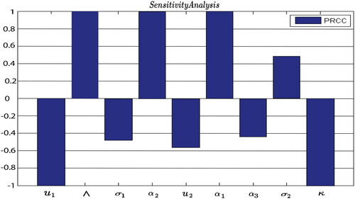
4. Sensitivity analysis of ${\mathcal{R}}_0^M$

Making decisions about effectively managing a disease necessitates careful consideration of the sensitivity analysis concept. The sensitivity analysis enables us to examine how variables fluctuate when the parameters in ${\mathcal{R}}_0^M$ are altered. It highlights the model’s most sensitive and impactful parameters and their effects on ${\mathcal{R}}_0^M.$

Definition 6.

(Zafar et al., 2022) The normalized forward sensitivity index (${\Gamma }_{\xi }$) of the basic reproduction number ${\mathcal{R}}_0^M$ that depends on a parameter $\xi$ is provided below as: (46) $${\Gamma }_{\xi }=\frac{\xi }{{\mathcal{R}}_0^M}\frac{\partial {\mathcal{R}}_0^M}{\partial \xi }.$$(46)

In order to investigate the sensitivity of ${\mathcal{R}}_0^M,$ we compute its derivatives as follows: $$\begin{array}{l}\frac{\partial {\mathcal{R}}_0^M}{\partial {\alpha }_1}=\frac{{\alpha }_2({\mu }_1+{\sigma }_2)\Lambda }{{\mu }_1({\alpha }_2+\kappa +{\mu }_1)({\mu }_2+{\alpha }_3+{\mu }_1)({\mu }_1+{\sigma }_1+{\sigma }_2)},\\ \frac{\partial {\mathcal{R}}_0^M}{\partial {\alpha }_2}=\frac{{\alpha }_1({\mu }_1+{\sigma }_2)\Lambda (\kappa +{\mu }_1)}{{\mu }_1{({\alpha }_2+\kappa +{\mu }_1)}^2({\mu }_2+{\alpha }_3+{\mu }_1)({\mu }_1+{\sigma }_1+{\sigma }_2)},\\ \frac{\partial {\mathcal{R}}_0^M}{\partial {\mu }_2}=-\frac{{\alpha }_1{\alpha }_2({\mu }_1+{\sigma }_2)\Lambda }{{\mu }_1({\alpha }_2+\kappa +{\mu }_1){({\mu }_2+{\alpha }_3+{\mu }_1)}^2({\mu }_1+{\sigma }_1+{\sigma }_2)},\\ \frac{\partial {\mathcal{R}}_0^M}{\partial \kappa }=-\frac{{\alpha }_1{\alpha }_2({\mu }_1+{\sigma }_2)\Lambda }{{\mu }_1{({\alpha }_2+\kappa +{\mu }_1)}^2({\mu }_2+{\alpha }_3+{\mu }_1)({\mu }_1+{\sigma }_1+{\sigma }_2)},\\ \frac{\partial {\mathcal{R}}_0^M}{\partial \Lambda }=\frac{{\alpha }_1{\alpha }_2({\mu }_1+{\sigma }_2)}{{\mu }_1({\alpha }_2+\kappa +{\mu }_1)({\mu }_2+{\alpha }_3+{\mu }_1)({\mu }_1+{\sigma }_1+{\sigma }_2)},\\ \frac{\partial {\mathcal{R}}_0^M}{\partial {\sigma }_1}=-\frac{{\alpha }_1{\alpha }_2({\mu }_1+{\sigma }_2)\Lambda }{{\mu }_1({\alpha }_2+\kappa +{\mu }_1)({\mu }_2+{\alpha }_3+{\mu }_1){({\mu }_1+{\sigma }_1+{\sigma }_2)}^2},\\ \frac{\partial {\mathcal{R}}_0^M}{\partial {\sigma }_2}=\frac{{\alpha }_1{\alpha }_2\Lambda {\sigma }_1}{{\mu }_1({\alpha }_2+\kappa +{\mu }_1)({\mu }_2+{\alpha }_3+{\mu }_1){({\mu }_1+{\sigma }_1+{\sigma }_2)}^2},\\ \frac{\partial {\mathcal{R}}_0^M}{\partial {\alpha }_3}=-\frac{{\alpha }_1{\alpha }_2({\mu }_1+{\sigma }_2)\Lambda }{{\mu }_1({\alpha }_2+\kappa +{\mu }_1){({\mu }_2+{\alpha }_3+{\mu }_1)}^2({\mu }_1+{\sigma }_1+{\sigma }_2)},\\ \frac{\partial {\mathcal{R}}_0^M}{\partial {\mu }_1}=-\frac{{\alpha }_1{\alpha }_2({\mu }_1+{\sigma }_2)\Lambda [\frac{{\sigma }_2({\alpha }_2+\kappa +2{\mu }_1)+{\mu }_1^2}{{\mu }_1({\mu }_1+{\sigma }_2)({\alpha }_2+\kappa +{\mu }_1)}+\frac{2{\mu }_1+{\sigma }_1+{\sigma }_2+{\mu }_2+{\alpha }_3}{({\mu }_2+{\alpha }_3+{\mu }_1)({\mu }_1+{\sigma }_1+{\sigma }_2)}]}{{\mu }_1({\alpha }_2+\kappa +{\mu }_1)({\mu }_2+{\alpha }_3+{\mu }_1)({\mu }_1+{\sigma }_1+{\sigma }_2)}.\end{array}$$

The normalized sensitivity indices of the involved parameters are obtained as: $$\begin{array}{cc}{\Gamma }_{{\alpha }_1}\hfill & =\frac{{\alpha }_1}{{\mathcal{R}}_0^M}\frac{\partial {\mathcal{R}}_0^M}{\partial {\alpha }_1}=1,\hfill \\ {\Gamma }_{\Lambda }\hfill & =\frac{\Lambda }{{\mathcal{R}}_0^M}\frac{\partial {\mathcal{R}}_0^M}{\Lambda }=1,\hfill \\ {\Gamma }_{{\alpha }_2}\hfill & =\frac{{\alpha }_2}{{\mathcal{R}}_0^M}\frac{{\mathcal{R}}_0^M}{\partial {\alpha }_2}=\frac{\kappa +{\mu }_1}{({\alpha }_2+\kappa +{\mu }_1)},\hfill \\ {\Gamma }_{{\mu }_2}\hfill & =\frac{{\mu }_2}{{\mathcal{R}}_0^M}\frac{\partial {\mathcal{R}}_0^M}{\partial {\mu }_2}=-\frac{{\mu }_2}{({\mu }_2+{\alpha }_3+{\mu }_1)},\hfill \\ {\Gamma }_{\kappa }\hfill & =\frac{\kappa }{{\mathcal{R}}_0^M}\frac{\partial {\mathcal{R}}_0^M}{\kappa }=-\frac{\kappa }{({\alpha }_2+\kappa +{\mu }_1)},\hfill \\ {\Gamma }_{{\sigma }_1}\hfill & =\frac{{\sigma }_1}{{\mathcal{R}}_0^M}\frac{\partial {\mathcal{R}}_0^M}{{\sigma }_1}=-\frac{{\sigma }_1}{({\mu }_1+{\sigma }_1+{\sigma }_2)},\hfill \\ {\Gamma }_{{\sigma }_2}\hfill & =\frac{{\sigma }_2}{{\mathcal{R}}_0^M}\frac{\partial {\mathcal{R}}_0^M}{{\sigma }_2}=\frac{{\sigma }_1{\sigma }_2}{({\mu }_1+{\sigma }_2)({\mu }_1+{\sigma }_1+{\sigma }_2)},\hfill \\ {\Gamma }_{{\alpha }_3}\hfill & =\frac{{\alpha }_3}{{\mathcal{R}}_0^M}\frac{\partial {\mathcal{R}}_0^M}{{\alpha }_3}=-\frac{{\alpha }_3}{({\mu }_2+{\alpha }_3+{\mu }_1)},\hfill \\ {\Gamma }_{{\mu }_1}\hfill & =\frac{{\mu }_1}{{\mathcal{R}}_0^M}\frac{\partial {\mathcal{R}}_0^M}{{\mu }_1}=-[\frac{{\sigma }_2({\alpha }_2+\kappa +2{\mu }_1)+{\mu }_1^2}{({\mu }_1+{\sigma }_2)({\alpha }_2+\kappa +{\mu }_1)}+\frac{{\mu }_1(2{\mu }_1+{\sigma }_1+{\sigma }_2+{\mu }_2+{\alpha }_3)}{({\mu }_2+{\alpha }_3+{\mu }_1)({\mu }_1+{\sigma }_1+{\sigma }_2)}].\hfill \end{array}$$

Table 3 and Figure 2 illustrate the positive impact of $\Lambda ,$ ${\alpha }_1,$ ${\alpha }_2,$ and ${\sigma }_2$ on the threshold parameter ${\mathcal{R}}_0^M,$ presenting that an increase in the parameter values would lead to a rise in ${\mathcal{R}}_0^M.$ It is clear from the calculated sensitivity indices that a 10$\%$ rise in the natality rate, effective contact rate, rate at which exposed humans become infected, and vaccine wane rate occurs to raise the value of ${\mathcal{R}}_0^M$ by 10$\%,$ 10$\%,$ 10$\%,$ and 4.8$\%,$ correspondingly, and can ultimately leading to a disease outbreak. Across the other perspective, natural recovery rate, natural death rate, death rate of infected humans due to measles, rate of vaccination of susceptible humans, and rate of exposed humans who have gone through screening and treatment suggests that raising their values by 10$\%$ will bring down the value of ${\mathcal{R}}_0^M$ by 4.3$\%,$ 10$\%,$ 5.6$\%,$ 4.8$\%,$ and 9.9$\%,$ respectively.

Figure 2. PRCC statistics regarding the significance of factors associated with ${\mathcal{R}}_0^M.$

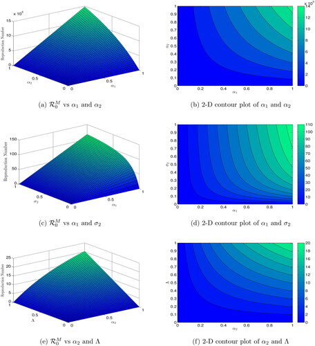
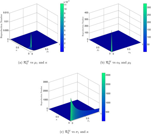
Figures (3–5) present the dynamics of reproduction numbers across various biological factors using 2D and 3D graphics. In Figure 3a, ${\mathcal{R}}_0^M$ is calculated as ${\alpha }_1$ and ${\alpha }_2$ increase, while all other parameters remain constant. Figure 3b shows a 2D contour plot of ${\alpha }_1$ versus ${\alpha }_2,$ indicating that an increase in ${\alpha }_1$ results in an increase in ${\alpha }_2.$ In Figure 3c, ${\mathcal{R}}_0^M$ is computed with ${\alpha }_1$ and ${\sigma }_2$ increasing. The 2D contour diagram of ${\alpha }_1$ versus ${\sigma }_2$ in Figure 3d illustrates that an increase in ${\alpha }_1$ leads to an increase in ${\sigma }_2.$ Figure 3e calculates ${\mathcal{R}}_0^M$ assuming ${\alpha }_2$ and $\Lambda$ are increasing, while the 2D contour graph of ${\alpha }_2$ versus $\Lambda$ in Figure 3f shows that an increase in ${\alpha }_2$ results in an increase in $\Lambda .$

Figure 3. The behaviours of ${\mathcal{R}}_0^M$ under different biological parameters.

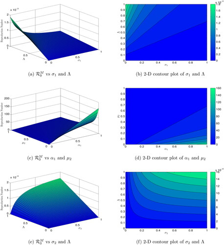
In the scenario where ${\sigma }_1$ decreases or $\Lambda$ increases, Figure 4a computes ${\mathcal{R}}_0^M.$ In Figure 4b, 2D contour maps of ${\sigma }_1$ versus $\Lambda$ confirm that a decrease in $\Lambda$ leads to an increase in ${\sigma }_1.$ Figure 4c calculates ${\mathcal{R}}_0^M$ assuming ${\alpha }_1$ is increasing and ${\mu }_2$ is decreasing. The 2D contour figure of ${\alpha }_1$ versus ${\mu }_2$ in Figure 4d shows that an increase in ${\alpha }_1$ causes a reduction in ${\mu }_2.$ Figure 4e computes ${\mathcal{R}}_0^M$ assuming ${\sigma }_2$ and $\Lambda$ are increasing, while the 2D contour plot of ${\alpha }_2$ versus $\Lambda$ in Figure 4f illustrates how an increase in ${\sigma }_2$ leads to an increase in $\Lambda .$

Figure 4. The behaviours of ${\mathcal{R}}_0^M$ under different biological parameters.

Finally, when $\kappa$ decreases or ${\mu }_1$ increases, Figure 5a determines ${\mathcal{R}}_0^M.$ Figure 5b calculates ${\mathcal{R}}_0^M$ with ${\alpha }_3$ and ${\mu }_2$ increasing, and Figure 5c displays similar performance trends.

Figure 5. The behaviours of ${\mathcal{R}}_0^M$ under different biological parameters.

5. Numerical analysis

This section introduces the Atangana-Toufik approach, a productive approximation method for the simulations of the considered system (2)(2) $$\{\begin{array}{ccc}{}_0^{\mathit{\text{ABC}}}{D}_t^{\vartheta }\mathbb{S}(t)\hfill & =\hfill & \Lambda -{\alpha }_1\mathbb{S}\mathbb{I}+{\sigma }_1\mathbb{V}-({\mu }_1+{\sigma }_2)\mathbb{S},\hfill \\ {}_0^{\mathit{\text{ABC}}}{D}_t^{\vartheta }\mathbb{V}(t)\hfill & =\hfill & {\sigma }_2\mathbb{S}-({\mu }_1+{\sigma }_1)\mathbb{V},\hfill \\ {}_0^{\mathit{\text{ABC}}}{D}_t^{\vartheta }\mathbb{E}(t)\hfill & =\hfill & {\alpha }_1\mathbb{S}\mathbb{I}-({\alpha }_2+\kappa +{\mu }_1)\mathbb{E},\hfill \\ {}_0^{\mathit{\text{ABC}}}{D}_t^{\vartheta }\mathbb{I}(t)\hfill & =\hfill & {\alpha }_2\mathbb{E}-({\mu }_2+{\alpha }_3+{\mu }_1)\mathbb{I},\hfill \\ {}_0^{\mathit{\text{ABC}}}{D}_t^{\vartheta }\mathbb{R}(t)\hfill & =\hfill & \kappa \mathbb{E}+{\alpha }_3\mathbb{I}-{\mu }_1\mathbb{R},\hfill \end{array}$$(2) . Remember that this strategy has previously been studied for fractional models (Butt et al., 2022; Toufik & Atangana, 2017). To apply this algorithm to system (2)(2) $$\{\begin{array}{ccc}{}_0^{\mathit{\text{ABC}}}{D}_t^{\vartheta }\mathbb{S}(t)\hfill & =\hfill & \Lambda -{\alpha }_1\mathbb{S}\mathbb{I}+{\sigma }_1\mathbb{V}-({\mu }_1+{\sigma }_2)\mathbb{S},\hfill \\ {}_0^{\mathit{\text{ABC}}}{D}_t^{\vartheta }\mathbb{V}(t)\hfill & =\hfill & {\sigma }_2\mathbb{S}-({\mu }_1+{\sigma }_1)\mathbb{V},\hfill \\ {}_0^{\mathit{\text{ABC}}}{D}_t^{\vartheta }\mathbb{E}(t)\hfill & =\hfill & {\alpha }_1\mathbb{S}\mathbb{I}-({\alpha }_2+\kappa +{\mu }_1)\mathbb{E},\hfill \\ {}_0^{\mathit{\text{ABC}}}{D}_t^{\vartheta }\mathbb{I}(t)\hfill & =\hfill & {\alpha }_2\mathbb{E}-({\mu }_2+{\alpha }_3+{\mu }_1)\mathbb{I},\hfill \\ {}_0^{\mathit{\text{ABC}}}{D}_t^{\vartheta }\mathbb{R}(t)\hfill & =\hfill & \kappa \mathbb{E}+{\alpha }_3\mathbb{I}-{\mu }_1\mathbb{R},\hfill \end{array}$$(2) in the sense of ABC derivative, let us assume a uniform mesh on the interval [0, T] with the nodes marked 0, 1, 2, ., Nh, where Nh is a positive integer and $h=\frac{T-0}{\mathit{\text{Nh}}}$ is the temporal step size. We now implement the Theorem 1 to each equation of the system (2)(2) $$\{\begin{array}{ccc}{}_0^{\mathit{\text{ABC}}}{D}_t^{\vartheta }\mathbb{S}(t)\hfill & =\hfill & \Lambda -{\alpha }_1\mathbb{S}\mathbb{I}+{\sigma }_1\mathbb{V}-({\mu }_1+{\sigma }_2)\mathbb{S},\hfill \\ {}_0^{\mathit{\text{ABC}}}{D}_t^{\vartheta }\mathbb{V}(t)\hfill & =\hfill & {\sigma }_2\mathbb{S}-({\mu }_1+{\sigma }_1)\mathbb{V},\hfill \\ {}_0^{\mathit{\text{ABC}}}{D}_t^{\vartheta }\mathbb{E}(t)\hfill & =\hfill & {\alpha }_1\mathbb{S}\mathbb{I}-({\alpha }_2+\kappa +{\mu }_1)\mathbb{E},\hfill \\ {}_0^{\mathit{\text{ABC}}}{D}_t^{\vartheta }\mathbb{I}(t)\hfill & =\hfill & {\alpha }_2\mathbb{E}-({\mu }_2+{\alpha }_3+{\mu }_1)\mathbb{I},\hfill \\ {}_0^{\mathit{\text{ABC}}}{D}_t^{\vartheta }\mathbb{R}(t)\hfill & =\hfill & \kappa \mathbb{E}+{\alpha }_3\mathbb{I}-{\mu }_1\mathbb{R},\hfill \end{array}$$(2) to get the numerical solutions of the proposed system, we obtain the following results: (47) $$\mathbb{S}(t)-\mathbb{S}(0)=\frac{1-\vartheta }{\mathcal{M}(\vartheta )}{\mathbb{G}}_1\left(t,\mathbb{S}(t)\right)+\frac{\vartheta }{\mathcal{M}(\vartheta )\Gamma (\vartheta )}{\int }_0^t{\mathbb{G}}_1(\rho ,\mathbb{S}(\rho )){(t-\rho )}^{\vartheta -1}d\rho .$$(47)

At a given point $t=t_{j+1},$ $j=0,1,2\dots ,$ then the Equation (47)(47) $$\mathbb{S}(t)-\mathbb{S}(0)=\frac{1-\vartheta }{\mathcal{M}(\vartheta )}{\mathbb{G}}_1\left(t,\mathbb{S}(t)\right)+\frac{\vartheta }{\mathcal{M}(\vartheta )\Gamma (\vartheta )}{\int }_0^t{\mathbb{G}}_1(\rho ,\mathbb{S}(\rho )){(t-\rho )}^{\vartheta -1}d\rho .$$(47) becomes $$\mathbb{S}(t_{j+1})-\mathbb{S}(0)=\frac{1-\vartheta }{\mathcal{M}(\vartheta )}{\mathbb{G}}_1\left(t_j,\mathbb{S}(t_j)\right)+\frac{\vartheta }{\mathcal{M}(\vartheta )\Gamma (\vartheta )}{\int }_{t_n}^{t_{n+1}}{\mathbb{G}}_1(\rho ,\mathbb{S}(\rho )){(t_{j+1}-\rho )}^{\vartheta -1}d\rho .$$

The above equation can written as: (48) $$\mathbb{S}(t_{j+1})-\mathbb{S}(0)=\frac{1-\vartheta }{\mathcal{M}(\vartheta )}{\mathbb{G}}_1\left(t_j,\mathbb{S}(t_j)\right)+\frac{\vartheta }{\mathcal{M}(\vartheta )\Gamma (\vartheta )}\sum _{n=0}^j{\int }_{t_n}^{t_{n+1}}{\mathbb{G}}_1(\rho ,\mathbb{S}(\rho )){(t_{j+1}-\rho )}^{\vartheta -1}d\rho .$$(48)

Applying two-step Lagrange polynomial interpolation on the function ${\mathbb{G}}_1(\rho ,\mathbb{S}(\rho ))$ in the interval $[t_j,t_{j+1}].$ Therefore, we obtain (49) $$\begin{array}{c}{\mathbb{S}}_{j+1}={\mathbb{S}}_0+\frac{1-\vartheta }{\mathcal{M}(\vartheta )}{\mathbb{G}}_1\left(t_j,{\mathbb{S}}_j\right)+\frac{\vartheta }{\mathcal{M}(\vartheta )\Gamma (\vartheta )}\sum _{n=0}^j\frac{{\mathbb{G}}_1(t_n,\mathbb{S}(t_n))}{h}{\int }_{t_n}^{t_{n+1}}(\rho -t_{n-1}){(t_{j+1}-\rho )}^{\vartheta -1}d\rho \\ \begin{array}{cc}-\hfill & \frac{{\mathbb{G}}_1(t_{n-1},\mathbb{S}(t_{n-1}))}{h}{\int }_{t_n}^{t_{n+1}}(\rho -t_n){(t_{j+1}-\rho )}^{\vartheta -1}d\rho ,\hfill \end{array}\end{array}$$(49) where $$\begin{array}{cc}{\Pi }_{n-1}\hfill & ={\int }_{t_n}^{t_{n+1}}(\rho -t_{n-1}){(t_{j+1}-\rho )}^{\vartheta -1}d\rho ,\hfill \\ \hfill & =\frac{h^{\vartheta +1}}{\vartheta (\vartheta +1)}[{\left(j+1-n\right)}^{\vartheta }\left(j-n+2+\vartheta \right)-{\left(j-n\right)}^{\vartheta }\left(j-n+2+2\vartheta \right)],\hfill \end{array}$$ and $$\begin{array}{cc}{\Pi }_n\hfill & ={\int }_{t_n}^{t_{n+1}}(\rho -t_n){(t_{j+1}-\rho )}^{\vartheta -1}d\rho ,\hfill \\ \hfill & =\frac{h^{\vartheta +1}}{\vartheta (\vartheta +1)}[{\left(j+1-n\right)}^{\vartheta +1}-{\left(j-n\right)}^{\vartheta }\left(j-n+1+\vartheta \right)].\hfill \end{array}$$

The above integrals substituted into the Equation (49)(49) $$\begin{array}{c}{\mathbb{S}}_{j+1}={\mathbb{S}}_0+\frac{1-\vartheta }{\mathcal{M}(\vartheta )}{\mathbb{G}}_1\left(t_j,{\mathbb{S}}_j\right)+\frac{\vartheta }{\mathcal{M}(\vartheta )\Gamma (\vartheta )}\sum _{n=0}^j\frac{{\mathbb{G}}_1(t_n,\mathbb{S}(t_n))}{h}{\int }_{t_n}^{t_{n+1}}(\rho -t_{n-1}){(t_{j+1}-\rho )}^{\vartheta -1}d\rho \\ \begin{array}{cc}-\hfill & \frac{{\mathbb{G}}_1(t_{n-1},\mathbb{S}(t_{n-1}))}{h}{\int }_{t_n}^{t_{n+1}}(\rho -t_n){(t_{j+1}-\rho )}^{\vartheta -1}d\rho ,\hfill \end{array}\end{array}$$(49) , then we have the solution $\mathbb{S}(t)$ as follows: (50) $$\begin{array}{cc}{\mathbb{S}}_{j+1}\hfill & ={\mathbb{S}}_0+\frac{1-\vartheta }{\mathcal{M}(\vartheta )}{\mathbb{G}}_1\left(t_j,{\mathbb{S}}_j\right)+\frac{\vartheta }{\mathcal{M}(\vartheta )\Gamma (\vartheta )}\sum _{n=0}^j[\frac{h^{\vartheta }{\mathbb{G}}_1(t_n,{\mathbb{S}}_n)}{\Gamma (\vartheta +2)}({\left(j+1-n\right)}^{\vartheta }\left(j-n+2+\vartheta \right)\hfill \\ \hfill & -{\left(j-n\right)}^{\vartheta }\left(j-n+2+2\vartheta \right))-\frac{h^{\vartheta }{\mathbb{G}}_1(t_{n-1},{\mathbb{S}}_{n-1})}{\Gamma (\vartheta +2)}\left({\left(j+1-n\right)}^{\vartheta +1}-{\left(j-n\right)}^{\vartheta }\left(j-n+1+\vartheta \right)\right)].\hfill \end{array}$$(50)

Similarly, for the other state variables, we evaluate the following schemes: (51) $$\begin{array}{c}{\mathbb{V}}_{j+1}={\mathbb{V}}_0+\frac{1-\vartheta }{\mathcal{M}(\vartheta )}{\mathbb{G}}_2\left(t_j,{\mathbb{V}}_j\right)+\frac{\vartheta }{\mathcal{M}(\vartheta )\Gamma (\vartheta )}\sum _{n=0}^j[\frac{h^{\vartheta }{\mathbb{G}}_2(t_n,{\mathbb{V}}_n)}{\Gamma (\vartheta +2)}({\left(j+1-n\right)}^{\vartheta }\left(j-n+2+\vartheta \right)\\ -{\left(j-n\right)}^{\vartheta }\left(j-n+2+2\vartheta \right))-\frac{h^{\vartheta }{\mathbb{G}}_2(t_{n-1},{\mathbb{V}}_{n-1})}{\Gamma (\vartheta +2)}\left({\left(j+1-n\right)}^{\vartheta +1}-{\left(j-n\right)}^{\vartheta }\left(j-n+1+\vartheta \right)\right)],\end{array}$$(51) (52) $$\begin{array}{c}{\mathbb{E}}_{j+1}={\mathbb{E}}_0+\frac{1-\vartheta }{\mathcal{M}(\vartheta )}{\mathbb{G}}_3\left(t_j,{\mathbb{E}}_j\right)+\frac{\vartheta }{\mathcal{M}(\vartheta )\Gamma (\vartheta )}\sum _{n=0}^j[\frac{h^{\vartheta }{\mathbb{G}}_3(t_n,{\mathbb{E}}_n)}{\Gamma (\vartheta +2)}({\left(j+1-n\right)}^{\vartheta }\left(j-n+2+\vartheta \right)\\ -{\left(j-n\right)}^{\vartheta }\left(j-n+2+2\vartheta \right))-\frac{h^{\vartheta }{\mathbb{G}}_3(t_{n-1},{\mathbb{E}}_{n-1})}{\Gamma (\vartheta +2)}\left({\left(j+1-n\right)}^{\vartheta +1}-{\left(j-n\right)}^{\vartheta }\left(j-n+1+\vartheta \right)\right)],\end{array}$$(52) (53) $$\begin{array}{c}{\mathbb{I}}_{j+1}={\mathbb{I}}_0+\frac{1-\vartheta }{\mathcal{M}(\vartheta )}{\mathbb{G}}_4\left(t_j,{\mathbb{I}}_j\right)+\frac{\vartheta }{\mathcal{M}(\vartheta )\Gamma (\vartheta )}\sum _{n=0}^j[\frac{h^{\vartheta }{\mathbb{G}}_4(t_n,{\mathbb{I}}_n)}{\Gamma (\vartheta +2)}({\left(j+1-n\right)}^{\vartheta }\left(j-n+2+\vartheta \right)\\ -{\left(j-n\right)}^{\vartheta }\left(j-n+2+2\vartheta \right))-\frac{h^{\vartheta }{\mathbb{G}}_4(t_{n-1},{\mathbb{I}}_{n-1})}{\Gamma (\vartheta +2)}\left({\left(j+1-n\right)}^{\vartheta +1}-{\left(j-n\right)}^{\vartheta }\left(j-n+1+\vartheta \right)\right)],\end{array}$$(53) (54) $$\begin{array}{c}{\mathbb{R}}_{j+1}={\mathbb{R}}_0+\frac{1-\vartheta }{\mathcal{M}(\vartheta )}{\mathbb{G}}_5\left(t_j,{\mathbb{R}}_j\right)+\frac{\vartheta }{\mathcal{M}(\vartheta )\Gamma (\vartheta )}\sum _{n=0}^j[\frac{h^{\vartheta }{\mathbb{G}}_5(t_n,{\mathbb{R}}_n)}{\Gamma (\vartheta +2)}({\left(j+1-n\right)}^{\vartheta }\left(j-n+2+\vartheta \right)\\ -{\left(j-n\right)}^{\vartheta }\left(j-n+2+2\vartheta \right))-\frac{h^{\vartheta }{\mathbb{G}}_5(t_{n-1},{\mathbb{R}}_{n-1})}{\Gamma (\vartheta +2)}\left({\left(j+1-n\right)}^{\vartheta +1}-{\left(j-n\right)}^{\vartheta }\left(j-n+1+\vartheta \right)\right)].\end{array}$$(54)

We perform some numerical simulations for the system (2)(2) $$\{\begin{array}{ccc}{}_0^{\mathit{\text{ABC}}}{D}_t^{\vartheta }\mathbb{S}(t)\hfill & =\hfill & \Lambda -{\alpha }_1\mathbb{S}\mathbb{I}+{\sigma }_1\mathbb{V}-({\mu }_1+{\sigma }_2)\mathbb{S},\hfill \\ {}_0^{\mathit{\text{ABC}}}{D}_t^{\vartheta }\mathbb{V}(t)\hfill & =\hfill & {\sigma }_2\mathbb{S}-({\mu }_1+{\sigma }_1)\mathbb{V},\hfill \\ {}_0^{\mathit{\text{ABC}}}{D}_t^{\vartheta }\mathbb{E}(t)\hfill & =\hfill & {\alpha }_1\mathbb{S}\mathbb{I}-({\alpha }_2+\kappa +{\mu }_1)\mathbb{E},\hfill \\ {}_0^{\mathit{\text{ABC}}}{D}_t^{\vartheta }\mathbb{I}(t)\hfill & =\hfill & {\alpha }_2\mathbb{E}-({\mu }_2+{\alpha }_3+{\mu }_1)\mathbb{I},\hfill \\ {}_0^{\mathit{\text{ABC}}}{D}_t^{\vartheta }\mathbb{R}(t)\hfill & =\hfill & \kappa \mathbb{E}+{\alpha }_3\mathbb{I}-{\mu }_1\mathbb{R},\hfill \end{array}$$(2) employing the values of the parameters from Table 2 as in a biologically feasible aspect to interpret our acquired results. The initial population of $\mathbb{S}(t),$ $\mathbb{V}(t),$ $\mathbb{E}(t),$ $\mathbb{I}(t),$ and $\mathbb{R}(t),$ are picked as 60309980, 0, 0, 76, and 0, respectively. The time varies between 0 and 25 months for the simulations. Population behaviour of the fractional measles model at the different fractional parameter values is depicted in Figure 6. Effect of fractional order values $\vartheta =0.80,0.84,0.88,0.92,0.96,1.00,$ on the solution behaviour of $\mathbb{S}(t),$ $\mathbb{V}(t),$ $\mathbb{E}(t),$ $\mathbb{I}(t),$ and $\mathbb{R}(t)$ is described in Figure 7. It is remarkable that when $\vartheta$ is equal to 1, then the dynamics of the proposed model achieved its integer order case. To assess the impact of varying fractional parameters on reducing measles prevalence in the general population, we analyze the effects of these parameters on individual subpopulations, as depicted in Figure 6. The results of the measles fractional model under various scenarios of fractional parameters are shown in Figure 6(a)-(f). Over time, the fractional parameter values increase, leading to a decrease in the subpopulations of susceptible, vaccinated, exposed, and infected individuals. Conversely, an increase in the fractional parameter values over time results in an increase in the number of recovered individuals. These response curves illustrate the stability and asymptotic behaviour of the measles fractional system.

Figure 6. Population behaviour of the measles fractional model at the different fractional parameter values.

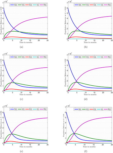
Figure 7. Simulations for the suggested model (2)(2) $$\{\begin{array}{ccc}{}_0^{\mathit{\text{ABC}}}{D}_t^{\vartheta }\mathbb{S}(t)\hfill & =\hfill & \Lambda -{\alpha }_1\mathbb{S}\mathbb{I}+{\sigma }_1\mathbb{V}-({\mu }_1+{\sigma }_2)\mathbb{S},\hfill \\ {}_0^{\mathit{\text{ABC}}}{D}_t^{\vartheta }\mathbb{V}(t)\hfill & =\hfill & {\sigma }_2\mathbb{S}-({\mu }_1+{\sigma }_1)\mathbb{V},\hfill \\ {}_0^{\mathit{\text{ABC}}}{D}_t^{\vartheta }\mathbb{E}(t)\hfill & =\hfill & {\alpha }_1\mathbb{S}\mathbb{I}-({\alpha }_2+\kappa +{\mu }_1)\mathbb{E},\hfill \\ {}_0^{\mathit{\text{ABC}}}{D}_t^{\vartheta }\mathbb{I}(t)\hfill & =\hfill & {\alpha }_2\mathbb{E}-({\mu }_2+{\alpha }_3+{\mu }_1)\mathbb{I},\hfill \\ {}_0^{\mathit{\text{ABC}}}{D}_t^{\vartheta }\mathbb{R}(t)\hfill & =\hfill & \kappa \mathbb{E}+{\alpha }_3\mathbb{I}-{\mu }_1\mathbb{R},\hfill \end{array}$$(2) using Atangan-Toufik scheme for the different values of fractional order $\vartheta .$

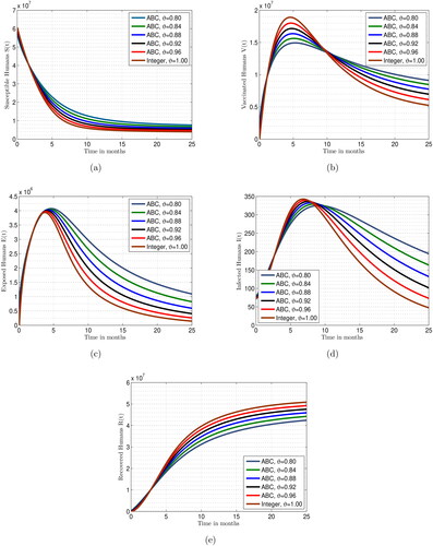
Table 2. Interpretation of involved symbols and their numeric values (47)(47) $$\mathbb{S}(t)-\mathbb{S}(0)=\frac{1-\vartheta }{\mathcal{M}(\vartheta )}{\mathbb{G}}_1\left(t,\mathbb{S}(t)\right)+\frac{\vartheta }{\mathcal{M}(\vartheta )\Gamma (\vartheta )}{\int }_0^t{\mathbb{G}}_1(\rho ,\mathbb{S}(\rho )){(t-\rho )}^{\vartheta -1}d\rho .$$(47) .

Symbol	Description	Value
$\Lambda$	Recruitment or natality rate of the population	7.27892$\times {10}^1$
${\alpha }_1$	Rate of effective contact of susceptible people	0.001
${\alpha }_2$	Rate at which exposed humans become infected	2.83562$\times {10}^{-5}$
${\alpha }_3$	Rate of natural recovery from infection	0.096
$\kappa$	Rate at which exposed humans who have gone through screening and treatment	1.45362
${\mu }_1$	Natural death rate of the population	$\frac{1}{(365\times 57.6)}$
${\mu }_2$	Death rate of infected humans due to measles	0.123
${\sigma }_1$	Rate of vaccination of susceptible humans	0.169
${\sigma }_2$	Rate of vaccine wane of the susceptible people	1.81656$\times {10}^{-1}$

Table 3. Sensitivity indices of ${\mathcal{R}}_0^M$ against the parameters.

Sensitivity index	Value	Sensitivity index	Value
${\Gamma }_{\Lambda }$	$+1.0000$	${\Gamma }_{{\mu }_2}$	$-0.5615$
${\Gamma }_{{\alpha }_1}$	$+1.0000$	${\Gamma }_{{\sigma }_1}$	$-0.4819$
${\Gamma }_{{\alpha }_2}$	$+1.0000$	${\Gamma }_{{\sigma }_2}$	$+0.4818$
${\Gamma }_{{\alpha }_3}$	$-0.4383$	${\Gamma }_{\kappa }$	$-0.9999$
${\Gamma }_{{\mu }_1}$	$-1.0001$	–	–

It seems that a larger fractional value leads to an improved outcome, as evidenced by the dynamics of the system approaching equilibrium in Figure 7(a)-(f) when the fractional order is reduced from 1 to 0.80 or even lower. Significant responses are observed in the compartments of the integrated model. Our numerical technique produces results as the time increment approaches a stable point, which represents the actual solution to the framework being studied. Each solution has a steady-state boundary. These graphs demonstrate how the model responds to decreasing fractional values, indicating that increasing the fractional value may enhance the solution’s accuracy.

This research illustrates that the long-lasting memory effect of the model can be effectively represented by fractional derivatives, which decrease as the fractional order $\vartheta$ approaches 1. The fractional differential operator captures an inherent effect, adding realism and accuracy to the proposed measles epidemic model. This framework considers long-term interdependencies, non-local consequences, durability, and recurrence, providing insights into measles transmission dynamics and guiding public health measures to prevent its spread. Decision-makers can utilize data relevant to the changing conditions of infected patients, as demonstrated by simulations. This analysis offers recommendations for practical measures to halt the spread of measles and anticipates advancements in this field.

6. Conclusion

The importance of epidemiological models in simulating disease transmission dynamics, fitting them to actual data, and recommending more effective control measures based on analysis cannot be overstated. To investigate the significance of memory in the system with the measles spread phenomenon, we have formulated an epidemiological framework for the spread of measles transmission with vaccination in a fractional context employing the ABC derivative. The primitive characteristics of the system, such as existence, uniqueness, boundedness, and positivity of the solution to the suggested fractional model, have been demonstrated using fundamental fractional calculus and fixed point theory. We have evaluated the system for equilibrium points and have used a next-generation matrix approach to obtain the threshold parameter for the considered model. To analyze the significance of various input components in ${\mathcal{R}}_0^M,$ we have conducted an analysis of the sensitivity of ${\mathcal{R}}_0^M$ using the partial rank correlation coefficient (PRCC) methodology. This analysis reveals that $\Lambda ,$ ${\alpha }_1,$ ${\alpha }_2,$ and ${\sigma }_2$ are the most sensitive factors. To control the spread of measles, we recommend minimizing or controlling these rates. Furthermore, a numerical approach for the stated fractional operator has been provided to depict the solution behaviour of the model. We have found that the complicated behaviour of the measles model can be addressed more accurately and effectively by the fractional-order model. The numerical results indicate that increasing the fractional parameter from 0.80 to 1 leads to an increase in the susceptibility and recovery of the measles population, while the infection rate in the population decreases over time. With these findings, we intend to actively engage with public health officials and clinicians to contribute to more beneficial epidemiological studies aimed at combating the epidemic. Future research will explore the transmission behaviour of measles using a newly designed fractal-fractional operator.

Acknowledgement

This work was supported by the Ministry of Education, Youth and Sports of the Czech Republic through the e-INFRA CZ (ID:90254).

Disclosure statement

No potential conflict of interest was reported by the author(s).

References

- Abbasi, Z., Zamani, I., Mehra, A. H. A., Shafieirad, M., & Ibeas, A. (2020). Optimal control design of impulsive SQEIAR epidemic models with application to COVID-19. Chaos, Solitons, and Fractals, 139, 110054. doi:10.1016/j.chaos.2020.110054
- Abboubakar, H., Fandio, R., Sofack, B. S., & Ekobena Fouda, H. P. (2022). Fractional dynamics of a measles epidemic model. Axioms, 11(8), 363. doi:10.3390/axioms11080363
- Ahmad, W., Rafiq, M., Butt, A. I. K., Ahmad, N., Ismaeel, T., Malik, S., … Asif, Z. (2024). Analytical and numerical explorations of optimal control techniques for the bi-modal dynamics of Covid-19. Nonlinear Dynamics, 112(5), 3977–4006. doi:10.1007/s11071-023-09234-8
- Ain, Q. T., Anjum, N., Din, A., Zeb, A., Djilali, S., & Khan, Z. A. (2022). On the analysis of Caputo fractional order dynamics of Middle East Lungs Coronavirus (MERS-CoV) model. Alexandria Engineering Journal, 61(7), 5123–5131. doi:10.1016/j.aej.2021.10.016
- Ain, Q. T., & Chu, Y. M. (2004). On fractal fractional hepatitis B epidemic model with modified vacci. New England Journal of Medicine, 351(27), 2832–2838.
- Ain, Q. T., Khan, A., Abdeljawad, T., Gómez-Aguilar, J. F., & Riaz, S. (2024). Dynamical study of varicella-zoster virus model in sense of Mittag-Leffler kernel. International Journal of Biomathematics, 17(03), 2350027. doi:10.1142/S1793524523500274
- Ain, Q. T., & Wang, J. (2023). A stochastic analysis of co-infection model in a finite carrying capacity population. International Journal of Biomathematics, 2350083. doi:10.1142/S1793524523500833
- Alzahrani, E. O., & Khan, M. A. (2020). Comparison of numerical techniques for the solution of a fractional epidemic model. The European Physical Journal Plus, 135(1), 110. doi:10.1140/epjp/s13360-020-00183-4
- Angelo, K. M., Gastañaduy, P. A., Walker, A. T., Patel, M., Reef, S., Lee, C. V., & Nemhauser, J. (2019). Spread of measles in Europe and implications for US travelers. Pediatrics, 144(1) doi:10.1542/peds.2019-0414
- Anjum, N., Ain, Q. T., & Li, X. X. (2021). Two-scale mathematical model for tsunami wave. GEM-International Journal on Geomathematics, 12(1), 10.
- Anjum, N., He, C. H., & He, J. H. (2021). Two-scale fractal theory for the population dynamics. Fractals, 29(07), 2150182. doi:10.1142/S0218348X21501826
- Baishya, C., Achar, S. J., Veeresha, P., & Prakasha, D. G. (2021). Dynamics of a fractional epidemiological model with disease infection in both the populations. Chaos (Woodbury, N.Y.), 31(4), 043130. doi:10.1063/5.0028905
- Batool, A., Talib, I., Riaz, M. B., & Tunç, C. (2022). Extension of lower and upper solutions approach for generalized nonlinear fractional boundary value problems. Arab Journal of Basic and Applied Sciences, 29(1), 249–256. doi:10.1080/25765299.2022.2112646
- Battegay, R., Itin, C., & Itin, P. (2012). Dermatological signs and symptoms of measles: A prospective case series and comparison with the literature. Dermatology (Basel, Switzerland), 224(1), 1–4. doi:10.1159/000335091
- Bohner, M., Tunç, O., & Tunç, C. (2021). Qualitative analysis of caputo fractional ıntegro-differential equations with constant delays. Computational and Applied Mathematics, 40(6), 2021–2214. doi:10.1007/s40314-021-01595-3
- Budigan Ni, H., de Broucker, G., Patenaude, B. N., Dudley, M. Z., Hampton, L. M., & Salmon, D. A. (2023). Economic impact of vaccine safety incident in Ukraine: The economic case for safety system investment. Vaccine, 41(1), 219–225.
- Butt, A. R., Ahmad Saqib, A., Alshomrani, A. S., Bakar, A., & Inc, M. (2024). Dynamical analysis of a nonlinear fractional cervical cancer epidemic model with the nonstandard finite difference method. Ain Shams Engineering Journal, 15(3), 102479. doi:10.1016/j.asej.2023.102479
- Butt, A. I. K., Ahmad, W., Rafiq, M., & Baleanu, D. (2022). Numerical analysis of Atangana-Baleanu fractional model to understand the propagation of a novel corona virus pandemic. Alexandria Engineering Journal, 61(9), 7007–7027. doi:10.1016/j.aej.2021.12.042
- Butt, A. R., Saqib, A. A., Bakar, A., Ozsahin, D. U., Ahmad, H., & Almohsen, B. (2023). Investigating the fractional dynamics and sensitivity of an epidemic model with nonlinear convex rate. Results in Physics, 54, 107089. doi:10.1016/j.rinp.2023.107089
- Callister, L. C. (2019). Global Measles Outbreak. MCN. The American Journal of Maternal Child Nursing, 44(4), 237. doi:10.1097/NMC.0000000000000542
- Center of Disease Control and Prevention. (2023). Global Measles Outbreaks. Available online: https://www.cdc.gov/globalhealth/ measles/data/global-measles-outbreaks.html. (accessed on 19 January 2023).
- Center of Disease Control and Prevention. (n.d.). Global Measles Outbreaks. Available online: https://www.cdc.gov/measles/cases-outbreaks.
- Conlan, A. J. K., Rohani, P., Lloyd, A. L., Keeling, M., & Grenfell, B. T. (2010). Resolving the impact of waiting time distributions on the persistence of measles. Journal of the Royal Society, Interface, 7(45), 623–640. doi:10.1098/rsif.2009.0284
- Din, A., Li, Y., Khan, F. M., Khan, Z. U., & Liu, P. (2022). On Analysis of fractional order mathematical model of Hepatitis B using Atangana-Baleanu Caputo (ABC) derivative. Fractals, 30(01), 2240017. doi:10.1142/S0218348X22400175
- Farman, M., Saleem, M. U., Ahmad, A., & Ahmad, M. O. (2018). Analysis and numerical solution of SEIR epidemic model of measles with non-integer time fractional derivatives by using Laplace Adomian Decomposition Method. Ain Shams Engineering Journal, 9(4), 3391–3397. doi:10.1016/j.asej.2017.11.010
- Fisker, A. B., Martins, J. S. D., Jensen, A. M., Martins, C., Aaby, P., & Thysen, S. M. (2022). Health effects of utilising hospital contacts to provide measles vaccination to children 9-59 months-a randomised controlled trial in Guinea-Bissau. Trials, 23(1), 349. doi:10.1186/s13063-022-06291-z
- Gambrell, A., Sundaram, M., & Bednarczyk, R. A. (2022). Estimating the number of US children susceptible to measles resulting from COVID-19-related vaccination coverage declines. Vaccine, 40(32), 4574–4579. doi:10.1016/j.vaccine.2022.06.033
- Gould, D. (2015). Measles: Symptoms, diagnosis, management and prevention. Primary Health Care, 25(1), 34–40. doi:10.7748/phc.25.1.34.e908
- Graef, J. R., Tunç, C., & Şevli, H. (2021). Razumikhin qualitative analyses of Volterra integro-fractional delay differential equation with Caputo derivatives. Communications in Nonlinear Science and Numerical Simulation, 103(2021), 106037. doi:10.1016/j.cnsns.2021.106037
- Ilesanmi, M. M., Adeyinka, D. A., & Olakunde, B. O. (2022). Sustainable Development Goals and childhood measles vaccination in Ekiti State, Nigeria: Results from spatial and interrupted time series analyses. Vaccine, 40(28), 3861–3868. doi:10.1016/j.vaccine.2022.05.037
- James Peter, O., Ojo, M. M., Viriyapong, R., & Abiodun Oguntolu, F. (2022). Mathematical model of measles transmission dynamics using real data from Nigeria. Journal of Difference Equations and Applications, 28(6), 753–770. doi:10.1080/10236198.2022.2079411
- Jost, M., Luzi, D., Metzler, S., Miran, B., & Mutsch, M. (2015). Measles associated with international travel in the region of the Americas, Australia and Europe, 2001-2013: A systematic review. Travel Medicine and Infectious Disease, 13(1), 10–18. doi:10.1016/j.tmaid.2014.10.022
- Khan, M. A., & Atangana, A. (2022). Mathematical modeling and analysis of COVID-19: A study of new variant Omicron. Physica A, 599, 127452. doi:10.1016/j.physa.2022.127452
- Khan, T., Ullah, Z., Ali, N., & Zaman, G. (2019). Modeling and control of the hepatitis B virus spreading using an epidemic model. Chaos, Solitons, Fractals, 124, 1–9. doi:10.1016/j.chaos.2019.04.033
- Liu, P., Ikram, R., Khan, A., & Din, A. (2022). The measles epidemic model assessment under real statistics: An application of stochastic optimal control theory. Computer Methods in Biomechanics and Biomedical Engineering, 26(2), 138–159. doi:10.1080/10255842.2022.2050222
- Memon, Z., Qureshi, S., & Memon, B. R. (2020). Mathematical analysis for a new nonlinear measles epidemiological system using real incidence data from Pakistan. European Physical Journal plus, 135(4), 378. doi:10.1140/epjp/s13360-020-00392-x
- Nabti, A., & Ghanbari, B. (2021). Global stability analysis of a fractional SVEIR epidemic model. Mathematical Methods in the Applied Sciences, 44(11), 8577–8597. doi:10.1002/mma.7285
- Ochoche, J. M., & Gweryina, R. I. (2014). A mathematical model of measles with vaccination and two phases of infectiousness. IOSR Journal of Mathematics, 10(1), 95–105. doi:10.9790/5728-101495105
- Peter, O. J., Qureshi, S., Ojo, M. M., Viriyapong, R., & Soomro, A. (2022). Mathematical dynamics of measles transmission with real data from Pakistan. Modeling Earth Systems and Environment, 9(2), 1545–1558. doi:10.1007/s40808-022-01564-7
- Pokharel, A., Adhikari, K., Gautam, R., Uprety, K. N., & Vaidya, N. K. (2022). Modeling transmission dynamics of measles in Nepal and its control with monitored vaccination program. Mathematical Biosciences and Engineering: MBE, 19(8), 8554–8579. doi:10.3934/mbe.2022397
- Qureshi, S., & Jan, R. (2021). Modeling of measles epidemic with optimized fractional order under Caputo differential operator. Chaos, Solitons, Fractals, 145, 110766. doi:10.1016/j.chaos.2021.110766
- Raza, N., Arshed, S., Bakar, A., Shahzad, A., & Inc, M. (2023). A numerical efficient splitting method for the solution of HIV time periodic reaction-diffusion model having spatial heterogeneity. Physica A: Statistical Mechanics and Its Applications, 609, 128385. doi:10.1016/j.physa.2022.128385
- Raza, N., Bakar, A., Khan, A., & Tunç, C. (2022). Numerical simulations of the fractional-order SIQ mathematical model of Corona virus disease using the nonstandard finite difference scheme. Malaysian Journal of Mathematical Sciences, 16(3), 391–411. doi:10.47836/mjms.16.3.01
- Samko, S. G., Kilbas, A. A., & Marichev, O. I. (1993). Fractional integrals and derivatives (Vol. 1). Yverdon, Yverdon-les-Bains, Switzerland: Gordon and Breach Science Publishers.
- Singh, J., Kumar, D., Hammouch, Z., & Atangana, A. (2018). A fractional epidemiological model for computer viruses pertaining to a new fractional derivative. Applied Mathematics and Computation, 316, 504–515. doi:10.1016/j.amc.2017.08.048
- Sowole, S. O., Ibrahim, A., Sangare, D., & Lukman, A. O. (2020). Mathematical model for measles disease with control on the susceptible and exposed compartments. Open Journal of Mathematical Analysis, 4(1), 60–75. doi:10.30538/psrp-oma2020.0053
- Tao, H., Anjum, N., & Yang, Y. J. (2023). The Aboodh transformation-based homotopy perturbation method: New hope for fractional calculus. Frontiers in Physics, 11, 1168795. doi:10.3389/fphy.2023.1168795
- Toufik, M., & Atangana, A. (2017). New numerical approximation of fractional derivative with non-local and non-singular kernel: Application to chaotic models. The European Physical Journal Plus, 132(10), 1–16. doi:10.1140/epjp/i2017-11717-0
- Tunç, C., Tunç, O., & Yao, J.-C. (2022). On the new qualitative results in integro-differential equations with Caputo fractional derivative and multiple kernels and delays. Journal of Nonlinear Convex Analysis, 23(11), 2577–2591.
- Tunç, O., & Tunç, C. (2023). Solution estimates to Caputo proportional fractional derivative delay integro –differential equations. Revista de la Real Academia de Ciencias Exactas, Fisicas y Naturales – Serie A: Matematicas 117(1). doi:10.1007/s13398-022-01345-y
- Tyagi, S., Gupta, S., Abbas, S., Das, K. P., & Riadh, B. (2021). Analysis of infectious disease transmission and prediction through SEIQR epidemic model. Nonautonomous Dynamical Systems, 8(1), 75–86. doi:10.1515/msds-2020-0126
- Uchaikin, V. V. (2013). Fractional derivatives for physicists and engineers (Vol. 2). Berlin: Springer
- Vojtek, I., Larson, H., Plotkin, S., & Van Damme, P. (2022). Evolving measles status and immunization policy development in six European countries. Human Vaccines & Immunotherapeutics, 18(1), 2031776. doi:10.1080/21645515.2022.2031776
- Yang, X. J. (2019). General fractional derivatives: Theory, methods and applications. Chapman and Hall/CRC.
- Zafar, Z. U. A., Zaib, S., Hussain, M. T., Tunç, C., & Javeed, S. (2022). Analysis and numerical simulation of tuberculosis model using different fractional derivatives. Chaos, Solitons and Fractals, 160, 112202. doi:10.1016/j.chaos.2022.112202
- Zafar, Z. U. L. A., Yusuf, A., Musa, S. S., Qureshi, S., Alshomrani, A. S., & Baleanu, D. (2022). Impact of public health awareness programs on COVID-19 dynamics: A fractional modeling approach. Fractals, 31(10) doi:10.1142/S0218348X23400054