Method to obtain parameters k₂, k₃ for dilution rate observer in AM2 model of the anaerobic digestion process in a batch reactor

ABSTRACT

Anaerobic digestion (AD) is a process of biochemical decomposition by anaerobic bacteria. Organic solid waste, subjected to anaerobic digestion, produces organic fertilizer and biogas, composed of methane, carbon dioxide, and other gases. The AM2 model describes the AD system and is the most widely used model for dynamic behavior analysis and control of AD processes. One of the most critical variables for system analysis is the concentration of volatile fatty acids (VFA). The behavior of the concentration of VFA depends on the dilution rate. This, in turn, depends on the performance parameters of producing and consuming VFA (k₂ and k₃). This paper presents a deterministic method to calculate the k₂ and k₃ parameters, from the dilution rate dynamics and Olson method for indirect validation of the parameters based on the direct validation of the concentration of VFA. Model results for VFA concentration showed an error of <0.4%. An error of <1.98% was found between the theoretical model and the experimental data. Overall, a global error of <2.37% gives a reliability to the proposed method to determine k₂ and k₃.

KEYWORDS:

• Anaerobic digestion
• observer D
• k2 and k3 parameters
• indirect validation
• dilution rate

Introduction

Anaerobic Digestion is a decomposition process through which bacteria break organic matter, such as food waste, without oxygen. The biochemical model described by (Liu et al. 2023) shows different products such as organic fertilizer, nutrients, bio-chemicals such as carboxylic acids, polyesters, proteins (Bolzonella et al. 2023), and biogas, which is mainly composed of carbon dioxide, CO₂ (25% to 45%), methane, CH₄ (50% to 70%), hydrogen sulfide (H₂S <1%), hydrogen (H₂), carbon monoxide CO and among others (Acosta-Pavas et al. 2023). Amongst these products, methane is has the most significant potential for energy production (Arshad et al. 2022; Kabeyi and Olanrewaju 2022).

Control of influencing factors is important to improve biogas production for electricity generation in AD (Olatunji, Madyira, and Adeleke 2023). The hydrogen and methane produced in both stages require the observability of an appreciable number of variables (Rodríguez-Mata et al. 2023), Some assumptions can simplify the variables used through a non-linear model for these two stages (Tawai, Sriariyanun, and Gentili 2022). Hence, the dynamics of the AD process have been studied through different mathematical models, such as anaerobic digestion model 2 (AM2) (Dekhici et al. 2022), which is a modification to the ADM1 (Mo et al. 2023). The AM2 model comprises six equations of state (Abdelhani and Samia 2022). In order to solve these differential equations and characterize the AD process, a first stage which consists of obtaining the value of the variables VFA concentration (S₂) and dilution rate (D), as well as the values of the production and consumption performance parameters during the process (k₁, k₂, k₃, k₄, k_5, and k₆) is required.

The D is not a measurable variable within the process. It reflects the relationship between the feed to the reactor and the volume of the mixture, which characterizes and regulates the production of VFA in the reaction mixture. Therefore, an observer is required to determine the value of D at different stages of the AD process.

The parameters k₁ to k₅ are obtained from the stoichiometric ratios of the AD process, which depend on the biochemical, biological, physicochemical, and physical characteristics of the substrate and the process.

The production of methane depends on the concentration of VFA. This behavior is reflected in the AM2 model through the parameters k₂ and k₃, which are related to production yield and VFA consumption yield, respectively. The unmeasurable D is estimated using an observer. The problem consists of obtaining the values of these parameters, particularly k₂ and k₃, which are the most challenging to obtain since they are related to the D. The difficulty lies in both securing and validating these parameters since they cannot be directly measured in the process. To address this, different authors use indirect instantaneous measurement of variables, such as VFA concentration, instead of employing a method to determine them in the dynamic model. This article presents a method for determining the parameters k₂ and k₃ and proposes an indirect validation strategy for the obtained values of k₂ and k₃ through experimental VFA concentration values.

Methodology

Determination of the parameters k₂ y k₃

To determine the parameters k₂ and k_3, an experiment was conducted to measure the system variables. In the case of k₂, the VFA substrate and the VFA production was measured. For the case of k₃, the VFA consumed and the methane produced from them are calculated.

Validation

The calculated value of k₂ and k₃ was validated indirectly through the direct validation of $S_2\left(\mathit{t}\right)$. For this purpose, the parameters k₂ and k₃ are incorporated into the AM2 model and, through numerical methods, theoretical $S_2\left(\mathit{t}\right)$ is obtained and then compared with values of $S_2\left(\mathit{t}\right)$ measured in the experiment. In this way, if the estimated value of $S_2\left(\mathit{t}\right)$ presents an error of less than 5% compared with the theoretical value of $S_2\left(\mathit{t}\right)$, calculated with k₂ and k₃, these parameters are validated with the above.

The indirect validation method for k₂ and k₃ can be summarized in five steps:

1. Measurement of $\mathit{TotalSolid}(\mathit{TS}),\mathit{TotalVolatilSolid}\left(\mathit{VS}\right),S_1\left(\mathit{t}\right),S_2\left(\mathit{t}\right),\mathit{C}{H}_4$

2. Calculation of parameters k₂ and k₃ starting from the variables measured in 1.

3. Construction of the theoretical model of $S_2\left(\mathit{t}\right)$ using the parameters of k₂ and k₃.

4. Construction of a theoretical model for $S_2\left(\mathit{t}\right)$ through the solution by numerical methods of the AM2 model using the parameters k₂ and k₃.

5. Comparison of the experimental $S_2\left(\mathit{t}\right)$ model vs. the theoretical model to establish the existing error between the two models.

AM2 dynamic model

The AM2 model is an adaptation of the Anaerobic Digestion Model No. 1 (Acosta-Pavas et al.2023), and (ADM1) (Ficara et al. 2012). The AM2 is simpler compared to ADM1 because it provides excellent features for the construction of solutions and includes variables to model the process dynamics, such as the VFA concentration, which influences the pH and the growth rate of methanogens (${\mu }_2$) (Kalyuzhnyi et al. 2002). There are other important variables for the analysis of the process, such as temperature (T), amount of feed substrate (S₁) (Bastin and Dochain 1991; Méndez-Acosta et al. 2016), the variation rate of S₁ $\left(\frac{d{S}_1}{\mathit{dt}}\right)$, the variation rate of S₂ $\left(\frac{d{S}_2}{\mathit{dt}}\right)$, the concentration of acidogenic bacteria $\left(X_1\right)$, the concentration of methanogenic bacteria (X₂), the growth rate of acidogenic bacteria $\left({\mu }_1\right)$, which have an impact on the volume of biogas and renewable energy produced and the methane flux (q_M), which can be assessed by Chemical Oxygen Demand (COD) or by volumetry.

On the other hand, the D and the chemical reaction rate (r₁) are parameters of great importance in the dynamic analysis of the process, where hydrogen and methane are the main products of AD (Chorukova et al. 2022; Pan et al. 2022).

(Stinga et al. 2017) proposed a control structure for the AD process to estimate variables through observers and include at least one observer, which can be the D and AD process is considered as a system with four stages.

The AM2 dynamic model of AD is built based on six state variables, these are:

a. Substrate concentration S₁, b. VFA concentration S₂, c. Concentration of acidogenic bacteria $X_1$, d. Concentration of methanogenic bacteria $X_2$, e. Alkalinity $\mathit{Z}$, f. Inorganic carbon concentration $\mathit{C}$

Other variables that intervene in the model and that are related to the previous ones are:

The growth rate of acidogenic bacteria $\left({\mu }_1\right)$, directly related to the concentration of acidogenic bacteria$X_1$. Growth rate of methanogenic bacteria $\left({\mu }_2\right)$,directly related to the concentration of methanogenic bacteria $X_2$. The available products are the volume of biogas (Salamanca-Valdivia et al. 2021) and the flow of methane (q_M).

The equations of state are developed based on biochemical and biological kinetics (Sun et al. 2023).

The stoichiometry presented in Table 1, reactions (a) to (e), are input to build the six state Equations (1)(1) $\frac{d{S}_1}{\mathit{dt}}=\mathit{D}\left(S_{1\mathit{in}}-S_1\right)-k_1{\mu }_1\left(S_1\right)X_1$(1) to (6(6) $\frac{\mathit{dC}}{\mathit{dt}}=\mathit{D}\left(C_{\mathit{in}}-\mathit{C}\right)-q_c+k_4{\mu }_1\left(S_1\right)X_1+k_5{\mu }_2\left(S_2\right)X_2$(6) ) that describe the dynamics of the AM2 model, together with the output Equation (7)(7) $q_M=k_6{\mu }_2\left(S_2\right)X_2$(7) .

(1) $\frac{d{S}_1}{\mathit{dt}}=\mathit{D}\left(S_{1\mathit{in}}-S_1\right)-k_1{\mu }_1\left(S_1\right)X_1$(1)

(2) $\frac{d{X}_1}{\mathit{dt}}=\left({\mu }_1\left(S_1\right)-\propto \mathit{D}\right)X_1$(2)

(3) $\frac{d{S}_2}{\mathit{dt}}=\mathit{D}\left(S_{2\mathit{in}}-S_2\right)+k_2{\mu }_1\left(S_1\right)X_1-k_3{\mu }_2\left(S_2\right)X_2$(3)

(4) $\frac{d{X}_2}{\mathit{dt}}=\left({\mu }_2\left(S_2\right)-\propto \mathit{D}\right)X_2$(4)

(5) $\frac{\mathit{dZ}}{\mathit{dt}}=\mathit{D}\left(Z_{\mathit{in}}-\mathit{Z}\right)$(5)

(6) $\frac{\mathit{dC}}{\mathit{dt}}=\mathit{D}\left(C_{\mathit{in}}-\mathit{C}\right)-q_c+k_4{\mu }_1\left(S_1\right)X_1+k_5{\mu }_2\left(S_2\right)X_2$(6)

(7) $q_M=k_6{\mu }_2\left(S_2\right)X_2$(7)

Table 1. Chemical reactions of the hydrolysis, acidogenesis, and methanogenesis phase.

Reaction	Phase
${\left(C_6{H}_{10}{O}_5\right)}_{\mathit{n}}+\mathit{n}{H}_2\mathit{O}\to \mathit{n}{C}_6{H}_{12}{O}_6$	$\left(\mathit{a}\right)\mathit{Hydrolysis}$
$\mathit{n}{C}_6{H}_{12}{O}_6\to 3\mathit{nC}{H}_3\mathit{COOH}$	$\left(\mathit{b}\right)\mathit{Acidogenesis}$
$C_6{H}_{12}{O}_6\to 2C_2{H}_5\mathit{OH}+2\mathit{C}{O}_2$	$\left(\mathit{c}\right)\mathit{Acidogenesis}$
$2C_2{H}_5\mathit{OH}+\mathit{C}{O}_2\to 2\mathit{C}{H}_3\mathit{COOH}+\mathit{C}{H}_4$	$\left(\mathit{d}\right)\mathit{Methanogenesis}$
$3\mathit{nC}{H}_3\mathit{COOH}\to 3\mathit{nC}{O}_2+3\mathit{nC}{H}_4$	$\left(\mathit{e}\right)\mathit{Methanogenesis}$

where: $S_1$ corresponds to the initial substrate, represented in the concentration of carbohydrates in the biodigestion mixture (g/L), $X_1$ corresponds to the biomass concentration (acidogenic bacteria, g/L), ${\mathit{S}}_2$ is the intermediate substrate, represented in the VFA (mg/L) concentration the biodigestion mixture. ${\mathbf{S}}_{2\mathit{in}}$ is the concentration of VFA (mg/L) present in the biodigestion mixture at the beginning of the AD process, ${\mathit{X}}_2$ corresponds to the biomass concentration (g/L) of methanogenic bacteria, $\mathit{Z}$, is the alkalinity represented as the sum of the concentration of acetate and bicarbonate in the mixture (meq/L), ${\mathit{k}}_{\mathit{i}}$ represents the activity constant of the reaction in each stage (production or consumption performance parameter), $q_M\mathit{\hspace{0.17em}}$corresponds to the methane flow produced (L/day).

Dilution rate observer

Observer´s model

By solving Eq. (3)(3) $\frac{d{S}_2}{\mathit{dt}}=\mathit{D}\left(S_{2\mathit{in}}-S_2\right)+k_2{\mu }_1\left(S_1\right)X_1-k_3{\mu }_2\left(S_2\right)X_2$(3) , D is obtained as stated in Equation (8)(8) $\mathit{D}=\left(\frac{1}{\left({\mathit{S}}_{2\mathit{in}}-S_2\right)}\right)\left(\frac{d{S}_2}{\mathit{dt}}-k_2{\mu }_1\left(S_1\right)X_1+k_3{\mu }_2\left(S_2\right)X_2\right)$(8) :

(8) $\mathit{D}=\left(\frac{1}{\left({\mathit{S}}_{2\mathit{in}}-S_2\right)}\right)\left(\frac{d{S}_2}{\mathit{dt}}-k_2{\mu }_1\left(S_1\right)X_1+k_3{\mu }_2\left(S_2\right)X_2\right)$(8)

The difficulty that arises in obtaining experimentally ${\mu }_1\left(S_1\right)X_1\mathrm{and}{\mu }_2\left(S_2\right)X_2$ in the continuous AD process, it is necessary to replace these Equation (8)(8) $\mathit{D}=\left(\frac{1}{\left({\mathit{S}}_{2\mathit{in}}-S_2\right)}\right)\left(\frac{d{S}_2}{\mathit{dt}}-k_2{\mu }_1\left(S_1\right)X_1+k_3{\mu }_2\left(S_2\right)X_2\right)$(8) variables with other variables that can be estimated from measurable variables (Lara-Cisneros and Dochain 2018).

Starting from Eq. (7)(7) $q_M=k_6{\mu }_2\left(S_2\right)X_2$(7) , we can solve for X₂ as shown in Equation ($9$):

(9) $X_2=\frac{q_M}{k_6{\mu }_2\left(S_2\right)}$(9)

Substituting in Eq. (8)(8) $\mathit{D}=\left(\frac{1}{\left({\mathit{S}}_{2\mathit{in}}-S_2\right)}\right)\left(\frac{d{S}_2}{\mathit{dt}}-k_2{\mu }_1\left(S_1\right)X_1+k_3{\mu }_2\left(S_2\right)X_2\right)$(8) the value obtained in (9), we have Equation (10)(10) $\mathit{D}=\left(\frac{1}{\left({\mathit{S}}_{2\mathit{in}}-S_2\right)}\right)\left(\frac{d{S}_2}{\mathit{dt}}-k_2{\mu }_1\left(S_1\right)X_1+k_3\frac{q_M}{K_6}\right)$(10) :

(10) $\mathit{D}=\left(\frac{1}{\left({\mathit{S}}_{2\mathit{in}}-S_2\right)}\right)\left(\frac{d{S}_2}{\mathit{dt}}-k_2{\mu }_1\left(S_1\right)X_1+k_3\frac{q_M}{K_6}\right)$(10)

This makes it possible to obtain the variables experimentally, except ${\mu }_1\left(S_1\right)X_1$, for which we proceed to estimate from other measurable variables$.$

Based on the reaction rate (r₁) of the S₁ substrate to produce S₂ and CO₂, in acidogenesis (Manjusha and Beevi 2016), Equation (11)(11) $r_1={\mu }_1\left(S_1\right)X_1\mathit{\hspace{0.17em}}$(11) is obtained:

(11) $r_1={\mu }_1\left(S_1\right)X_1\mathit{\hspace{0.17em}}$(11)

Then, substituting $r_1$ for ${\mu }_1\left(S_1\right)X_1$ in Equation (10)(10) $\mathit{D}=\left(\frac{1}{\left({\mathit{S}}_{2\mathit{in}}-S_2\right)}\right)\left(\frac{d{S}_2}{\mathit{dt}}-k_2{\mu }_1\left(S_1\right)X_1+k_3\frac{q_M}{K_6}\right)$(10) gives Equation (12)(12) $\mathit{D}=\left(\frac{1}{\left({\mathit{S}}_{2\mathit{in}}-S_2\right)}\right)\left(\frac{d{S}_2}{\mathit{dt}}-k_2{r}_1+k_3\frac{q_M}{K_6}\right)$(12) :

(12) $\mathit{D}=\left(\frac{1}{\left({\mathit{S}}_{2\mathit{in}}-S_2\right)}\right)\left(\frac{d{S}_2}{\mathit{dt}}-k_2{r}_1+k_3\frac{q_M}{K_6}\right)$(12)

To solve Equation (12)(12) $\mathit{D}=\left(\frac{1}{\left({\mathit{S}}_{2\mathit{in}}-S_2\right)}\right)\left(\frac{d{S}_2}{\mathit{dt}}-k_2{r}_1+k_3\frac{q_M}{K_6}\right)$(12) , it is required that the variables $S_2,r_1,q_M,$ be observable in the process (Draa et al. 2018).

The use of a linearized control (Draa et al. 2015) is therefore proposed, through Equation (13)(13) $\frac{d{q}_M^{\ast }-q_M}{\mathit{dt}}+\mathit{\lambda }\left(q_M^{\ast }-q_M\right)=0$(13) :

(13) $\frac{d{q}_M^{\ast }-q_M}{\mathit{dt}}+\mathit{\lambda }\left(q_M^{\ast }-q_M\right)=0$(13)

where λ is the controllable operator.

Using Equation (7)(7) $q_M=k_6{\mu }_2\left(S_2\right)X_2$(7) , the change in the methane flux can be expressed by Equation (14)(14) $\frac{d{q}_M}{\mathit{dt}}=k_6\frac{d{\mu }_2\left(S_2\right)}{\mathit{dt}}{X}_2+k_6{\mu }_2\left(S_2\right)\frac{d{X}_2}{\mathit{dt}}$(14) :

(14) $\frac{d{q}_M}{\mathit{dt}}=k_6\frac{d{\mu }_2\left(S_2\right)}{\mathit{dt}}{X}_2+k_6{\mu }_2\left(S_2\right)\frac{d{X}_2}{\mathit{dt}}$(14)

Substituting the Equation of state (4) in Eq. (14)(14) $\frac{d{q}_M}{\mathit{dt}}=k_6\frac{d{\mu }_2\left(S_2\right)}{\mathit{dt}}{X}_2+k_6{\mu }_2\left(S_2\right)\frac{d{X}_2}{\mathit{dt}}$(14) we have Equation (15)(15) $\frac{d{q}_M}{\mathit{dt}}=k_6\frac{d{\mu }_2\left(S_2\right)}{\mathit{dt}}{X}_2+q_M\left({\mu }_2\left(S_2\right)-\propto \mathit{D}\right)$(15) :

(15) $\frac{d{q}_M}{\mathit{dt}}=k_6\frac{d{\mu }_2\left(S_2\right)}{\mathit{dt}}{X}_2+q_M\left({\mu }_2\left(S_2\right)-\propto \mathit{D}\right)$(15)

The Equation (15)(15) $\frac{d{q}_M}{\mathit{dt}}=k_6\frac{d{\mu }_2\left(S_2\right)}{\mathit{dt}}{X}_2+q_M\left({\mu }_2\left(S_2\right)-\propto \mathit{D}\right)$(15) can be expressed as shown in Equation (16)(16) $\frac{d{q}_M}{\mathit{dt}}=q_M\left[\frac{\left(k_{S_2}{k}_{I_2}-{S_2}^2\right){\mu }_2\left(S_2\right)}{k_{I_2}{\mu }_{2\mathit{max}}{S_2}^2}\right]\left(\mathit{D}\left(S_{2,\mathit{in}}-S_2\right)+k_2{r}_1-\frac{k_3}{k_6}{q}_M\right)+q_M\left({\mu }_2\left(S_2\right)-\propto \mathit{D}\right)$(16) :

(16) $\frac{d{q}_M}{\mathit{dt}}=q_M\left[\frac{\left(k_{S_2}{k}_{I_2}-{S_2}^2\right){\mu }_2\left(S_2\right)}{k_{I_2}{\mu }_{2\mathit{max}}{S_2}^2}\right]\left(\mathit{D}\left(S_{2,\mathit{in}}-S_2\right)+k_2{r}_1-\frac{k_3}{k_6}{q}_M\right)+q_M\left({\mu }_2\left(S_2\right)-\propto \mathit{D}\right)$(16)

Since the reference value is constant ($q_M^{\ast }$=constant), Equation (17)(17) $\mathit{\lambda }\left(q_M^{\ast }-q_M\right)=\frac{d{q}_M}{\mathit{dt}}=q_M\left[\frac{\left(k_{S_2}{k}_{I_2}-{S_2}^2\right){\mu }_2\left(S_2\right)}{k_{I_2}{\mu }_{2\mathit{max}}{S_2}^2}\right]\left(\mathit{D}\left(S_{2,\mathit{in}}-S_2\right)+k_2{r}_1-\frac{k_3}{k_6}{q}_M\right)+q_M\left({\mu }_2\left(S_2\right)-\propto \mathit{D}\right)$(17) is obtained:

(17) $\mathit{\lambda }\left(q_M^{\ast }-q_M\right)=\frac{d{q}_M}{\mathit{dt}}=q_M\left[\frac{\left(k_{S_2}{k}_{I_2}-{S_2}^2\right){\mu }_2\left(S_2\right)}{k_{I_2}{\mu }_{2\mathit{max}}{S_2}^2}\right]\left(\mathit{D}\left(S_{2,\mathit{in}}-S_2\right)+k_2{r}_1-\frac{k_3}{k_6}{q}_M\right)+q_M\left({\mu }_2\left(S_2\right)-\propto \mathit{D}\right)$(17)

Solving Equation (17)(17) $\mathit{\lambda }\left(q_M^{\ast }-q_M\right)=\frac{d{q}_M}{\mathit{dt}}=q_M\left[\frac{\left(k_{S_2}{k}_{I_2}-{S_2}^2\right){\mu }_2\left(S_2\right)}{k_{I_2}{\mu }_{2\mathit{max}}{S_2}^2}\right]\left(\mathit{D}\left(S_{2,\mathit{in}}-S_2\right)+k_2{r}_1-\frac{k_3}{k_6}{q}_M\right)+q_M\left({\mu }_2\left(S_2\right)-\propto \mathit{D}\right)$(17) , the D is expressed as Equation (18)(18) $\mathit{D}=\frac{\frac{\lambda \left(q_M^{\ast }-q_M\right)}{q_M\mathit{\beta }}-k_2{r}_1+\frac{k_3}{k_6}{q}_M-\frac{{\mu }_2\left(S_2\right)}{\mathit{\beta }}}{\left(S_{2,\mathit{in}}-S_2\right)-\frac{\propto }{\beta }}$(18) , where $\mathit{\beta }=\left[\frac{\left(k_{S_2}{k}_{I_2}-{S_2}^2\right){\mu }_2\left(S_2\right)}{k_{I_2}{\mu }_{2\mathit{max}}{S_2}^2}\right]$:

(18) $\mathit{D}=\frac{\frac{\lambda \left(q_M^{\ast }-q_M\right)}{q_M\mathit{\beta }}-k_2{r}_1+\frac{k_3}{k_6}{q}_M-\frac{{\mu }_2\left(S_2\right)}{\mathit{\beta }}}{\left(S_{2,\mathit{in}}-S_2\right)-\frac{\propto }{\beta }}$(18)

Determination of $K_2\mathit{and}{K}_3$ parameters

The procedure to determine the parameters $k_2\mathrm{and}{k}_3$ is carried out utilizing the following steps, where $k_2:$ VFA production yield (mmol/g); $k_3:$ VFA consumption yield (mmol/g):

1. Measurement of moles of VFA produced.

2. Calculation of the VFA production yield parameter, $k_2$.

3. Calculation of moles of methane produced.

4. Calculation of VFA consumption yield parameter, ${\mathit{k}}_3$.

5. Validation of$k_2\mathit{\hspace{0.17em}}\mathrm{and}\mathit{\hspace{0.17em}}{k}_3$ parameters.

The steps of the procedure in this case study are carried out below.

a) Step 1 VFA mole measurement

Experiment 1. Alkalinity, total solids, total volatile solids, and methane.

Experiment 1 is carried out in a batch reactor, as shown in Supplementary material S1. The results obtained are, TS, VS, substrate concentration $S_1$, Alkalinity Z, ammonium content in the mixture, ammonium content in the activated sludge, the volume of biogas, and volume of $\mathit{C}{H}_4$.

The measurement of the alkalinity variables, $S_2,S_1,q_M$ was carried out to determine the values of $k_2$and $k_3$and build the model for $S_2\left(\mathit{t}\right)$.

To measure the variables alkalinity, carbohydrate concentration $\left(S_1\right)$, VFA $\left(S_2\right)$, methane flux ($q_M$), pH, and temperature, the following techniques were used: The reaction rate of VFA is established from the stoichiometric ratio, as shown in Equation (16)(16) $\frac{d{q}_M}{\mathit{dt}}=q_M\left[\frac{\left(k_{S_2}{k}_{I_2}-{S_2}^2\right){\mu }_2\left(S_2\right)}{k_{I_2}{\mu }_{2\mathit{max}}{S_2}^2}\right]\left(\mathit{D}\left(S_{2,\mathit{in}}-S_2\right)+k_2{r}_1-\frac{k_3}{k_6}{q}_M\right)+q_M\left({\mu }_2\left(S_2\right)-\propto \mathit{D}\right)$(16) (Gavala, Angelidaki, and Ahring 2003). Alkalinity was also measured by titration following the methodology stablished in (APHA-AWWA-WPCF 2017). Volumetric analysis was used to determine the methane concentration. Likewise, carbohydrates are valued by the spectrometry technique at 492 nm following the method of (DuBois et al. 1956), pH is measured continuously through the transducer and the data acquisition and processing system directly within the digestion mixture (Hajji et al. 2016).

Subsequently, ammonium titration is carried out since ammonium in concentrations higher than 400 mg/L becomes an inhibitor of bacterial growth. In the experiment, it was found that the ammonium concentration was below the minimum inhibition concentration. Since that does not alter bacterial growth, it is not subject to further analysis. The results are presented in Table 2.

Table 2. Experimental data obtained in test 1.

COMPOUND	SAMPLE CONTENT
Biogas	107.7 ml/100 g of OSW
Methane	75 ml/100 g of OSW
Ammonium	327 mg/L In Biodigester
Ammonium	230 mg/L Active Sludge
Carbohydrates (S1)	$85.47\mathit{\%}$ In TS
Alkalinity	10–8 mg/ml CO3
Lipids	1–28% OSW total
TS	307.41 g/Kg OSW
VS	300.63 g/Kg OSW

TS are determined by dehydration at 105°C to obtain 307.41 g/L, and VS of 300.63 g/L are measured by calculating the TS at 550°C.

The substrate concentration is determined as the carbohydrate content in the TS.

Typically, the carbohydrate concentration is calculated using a phenol solution in the presence of sulfuric acid, generating an orange color. It is measured by colorimetry with a wavelength of 492 nm. The percentage of carbohydrates is determined from Equation (19)(19) $\mathrm{\%Carb}{s}_{\mathit{Total}}=\frac{\left(\mathit{m}\ast \mathit{Ab}{\mathit{s}}_{492}\left(\mathit{nm}\right)+\mathit{b}\right)\ast V_e}{V_m\ast W_b}\ast 100$(19) .

(19) $\mathrm{\%Carb}{s}_{\mathit{Total}}=\frac{\left(\mathit{m}\ast \mathit{Ab}{\mathit{s}}_{492}\left(\mathit{nm}\right)+\mathit{b}\right)\ast V_e}{V_m\ast W_b}\ast 100$(19)

where: $\mathit{m}$ is the slope of the linear Equation with a value of 0.016, $\mathit{Ab}{s}_{492}$ (nm) is the absorbance value, $\mathit{b}$ is the ordinate to the origin of the linear Equation with the value of 0.0411, $V_e$ is the total volume of the acid extract, in ml, $V_m$ is the volume of aliquot to be tested, in ml, and $W_b$ is the weight of dry lyophilized biomass, in mg.

(20) $\mathrm{\%Carb}{s}_{\mathit{Total}}=\frac{\left(0.016\ast 0.368+0.0411\right)\ast 0.064L}{{10}^{-4}\mathit{L}\ast 22\mathit{mg}}\ast 100=85.47\mathrm{\%}$(20)

This resulting value corresponds to the percentage content of organic material in the TS.

The titration of methane is carried out by volumetric titration using a $\mathit{C}{O}_2$ trap through which the produced biogas passes. A total of 150 ml of $\mathit{C}{H}_4$ was produced in 15 days from 200 g of organic solid waste (OSW).

Using the ideal gas law, the methane equivalents produced is calculated as given in Equation (21)(21) $\mathit{n}=\frac{1\mathit{atm}\ast 0,15\mathit{L}}{0,08205\left[\frac{\mathit{atm}\ast \mathit{L}}{mol{\ast }^{\circ }\mathit{K}}\right]\ast {293}^{\circ }\mathit{K}}=6.138\mathit{mmol}\mathit{de}\mathit{C}{H}_4$(21) :

(21) $\mathit{n}=\frac{1\mathit{atm}\ast 0,15\mathit{L}}{0,08205\left[\frac{\mathit{atm}\ast \mathit{L}}{mol{\ast }^{\circ }\mathit{K}}\right]\ast {293}^{\circ }\mathit{K}}=6.138\mathit{mmol}\mathit{de}\mathit{C}{H}_4$(21)

The total alkalinity was calculated as calcium carbonate (CaCO₃), expressed in mg L⁻¹ as shown in Equation (22)(22) $\mathit{CaC}{O}_3=\frac{PE\ast N_i\ast V_g}{V_m}\ast 1000$(22) :

(22) $\mathit{CaC}{O}_3=\frac{PE\ast N_i\ast V_g}{V_m}\ast 1000$(22)

Where: $\mathit{PE}$ is the equivalent weight at CaCO₃ to convert Eq/L to mg, $N_i$ is the initial normal concentration of H₂SO₄, $V_g$ is the total volume of H₂SO₄ expended in the titration (L), and $V_m$ is the sample volume (L). It is obtained: 10.8 mg (represented as carbonate)/ml

Calculation of the VFA production yield parameters K₂

Experiment 2. VFA concentration, S₂(t)

The second experiment consists of two batch-type reactors with identical conditions, temperature control, and aluminum covering to avoid the incidence of direct light on the process, activated using a mixture of organic solid waste with active sludge in a 1:3 S:I ratio. The tests were carried out for 21 days, with a temperature system at 37°C ±1°C. VFA measurement is made by titration. Table 3 shows the data of the measurements.

Table 3. Experimental data obtained in test 2.

TIME	TS (g/kg OSW)	S2(t) mmol VFA/ml	mg/ml VFA
Day 1	319	1.46	87.6
Day 2	319	1.68	100.8
Day 3	319	1.75	105
Day 4	319	1.72	103.2
Day 5	319	1.62	95.2
Day 6	319	1.52	91.2
Day 7	319	1.47	88.2
Day 8	319	1.42	85.2

The estimation of the parameters k₂ and k₃ are carried out from measurements made of the variables S₁, S₂, biogas flow, and CH₄ concentration (Tables 2 and 3) in the biogas as referred in Dittmer, Krümpel, and Lemmer (2021) and Salgado (2019).

b) Step: 2 calculation of VFA production yield parameter, K₂

From the results obtained in the experimental phase, the VFA production yield parameter $k_2$is calculated.

The production yield of VFA in acidogenesis corresponding to k₂ is given in mmol of VFA produced (S₂) divided by the weight in g. of initial substrate (S₁). The data obtained can be seen in Table 3.

The measured number of moles from titration is 1.75 mmol VFA/ml. The biodigester mixture has a volume of 904 ml, hence, the total amount of VFA is calculated as given in Eq. 23(23) $n_{\left(C{H}_3\mathit{COOH}\right)}=\frac{1.75\mathit{mmol}\mathit{VFA}}{\mathit{ml}\mathit{mixture}}\ast 904\mathit{ml}\mathit{mixture}=1582\mathit{mmol}\mathit{de}\mathit{VFA}$(23) .

(23) $n_{\left(C{H}_3\mathit{COOH}\right)}=\frac{1.75\mathit{mmol}\mathit{VFA}}{\mathit{ml}\mathit{mixture}}\ast 904\mathit{ml}\mathit{mixture}=1582\mathit{mmol}\mathit{de}\mathit{VFA}$(23)

The amount of Total Volatile Solids (VS) in the mixture was 6.252 g, so the k₂ parameter is calculated as shown in Eq. (24)(24) $k_2=\frac{1582\mathit{mmol}\mathit{de}\mathit{VFA}}{6.252\mathit{g}\mathit{de}\mathit{STV}}=252.63\mathit{mmol}\mathit{de}\mathit{VFA}/\mathit{g}\mathit{de}\mathit{STV}$(24) .

(24) $k_2=\frac{1582\mathit{mmol}\mathit{de}\mathit{VFA}}{6.252\mathit{g}\mathit{de}\mathit{STV}}=252.63\mathit{mmol}\mathit{de}\mathit{VFA}/\mathit{g}\mathit{de}\mathit{STV}$(24)

c) Step 3. Calculation of methane moles

The consumption yield of VFA in methanogenesis (see Table 1 for balanced chemical equation), corresponding to $k_3$ is given in mmol of VFA (S₂) consumed or in methane produced by weight in g of VFA in the substrate S₂. The data on the methane produced can be seen in Table 2.

To calculate the methane yield from the volume obtained, the number of moles produced is calculated using the ideal gas law as shown in Eq. (25)(25) $V_{C{H}_4}=\frac{n\ast R\ast T^{\circ }}{\mathit{P}}\mathit{therefore},\mathit{n}=\frac{P\ast VC{H}_4}{\mathit{R}\ast T^{\circ }}=\frac{1\mathit{atm}\ast 0.15\mathit{L}}{0.082\frac{\mathit{atm}\ast \mathit{L}}{mol{\ast }^{\circ }\mathit{K}}\ast {298}^{\circ }\mathit{K}}=6.138\mathit{mmol}\mathit{C}{H}_4$(25) :

(25) $V_{C{H}_4}=\frac{n\ast R\ast T^{\circ }}{\mathit{P}}\mathit{therefore},\mathit{n}=\frac{P\ast VC{H}_4}{\mathit{R}\ast T^{\circ }}=\frac{1\mathit{atm}\ast 0.15\mathit{L}}{0.082\frac{\mathit{atm}\ast \mathit{L}}{mol{\ast }^{\circ }\mathit{K}}\ast {298}^{\circ }\mathit{K}}=6.138\mathit{mmol}\mathit{C}{H}_4$(25)

d) Step 4. Calculation of VFA consumption performance parameter, k_3.

AGV consumption performance ($k_3$), is calculated as shown in Eq. (26)(26) $k_3=6.138\frac{\mathrm{mmol}C{H}_4}{0.0894\mathit{g}\mathit{VFA}}=68.65\frac{\mathrm{mmol}C{H}_4}{\mathit{g}\mathit{VFA}}$(26) $:$

(26) $k_3=6.138\frac{\mathrm{mmol}C{H}_4}{0.0894\mathit{g}\mathit{VFA}}=68.65\frac{\mathrm{mmol}C{H}_4}{\mathit{g}\mathit{VFA}}$(26)

where 6.138 mmol of $\mathit{C}{H}_4$ is the amount produced per day and 0.0894 g of VFA is the amount consumed per day. With the values of the parameters $k_2\mathrm{and}{k}_3$ calculated, the mathematical model of Eq. (18)(18) $\mathit{D}=\frac{\frac{\lambda \left(q_M^{\ast }-q_M\right)}{q_M\mathit{\beta }}-k_2{r}_1+\frac{k_3}{k_6}{q}_M-\frac{{\mu }_2\left(S_2\right)}{\mathit{\beta }}}{\left(S_{2,\mathit{in}}-S_2\right)-\frac{\propto }{\beta }}$(18) is completed. Hence, we can generate an equation for the observer of the D with which the variables are obtained for the AM2 model as expressed in Equation (27)(27) $\mathit{D}=\frac{\frac{\lambda \left(q_M^{\ast }-q_M\right)}{q_M\mathit{\beta }}-252.63r_1+\frac{68.65}{k_6}{q}_M-\frac{{\mu }_2\left(S_2\right)}{\mathit{\beta }}}{\left(S_{2,\mathit{in}}-S_2\right)-\frac{\propto }{\beta }}$(27) .

(27) $\mathit{D}=\frac{\frac{\lambda \left(q_M^{\ast }-q_M\right)}{q_M\mathit{\beta }}-252.63r_1+\frac{68.65}{k_6}{q}_M-\frac{{\mu }_2\left(S_2\right)}{\mathit{\beta }}}{\left(S_{2,\mathit{in}}-S_2\right)-\frac{\propto }{\beta }}$(27)

e) Step 5. Validation

To perform the validation of the parameters $k_2\mathrm{and}{k}_3$, first the experimental model of $S_2\left(\mathit{t}\right)$ was built based on the measured values of $S_2\left(\mathit{t}\right)$. Subsequently, the theoretical model of $S_2\left(\mathit{t}\right)$ was obtained from the AM2 model where the previously calculated values of $k_2\mathrm{and}{k}_3$ have been replaced. The direct validation of the theoretical model of $S_2\left(\mathit{t}\right)$ is obtained through the error calculated with Eqs. (28)(28) $e_i=\frac{{\mathit{D}}_{\mathit{Ti}}-D_{\mathit{Ei}}}{D_{\mathit{Ei}}}\ast 100\mathrm{\%}$(28) and (29(29) $e_E=\sqrt[2]{\frac{1}{n}\sum _{\mathit{i}=1}^n{e_i}^2}$(29) ), which allows the values of $k_2\mathrm{and}{k}_3$ to be validated indirectly.

(28) $e_i=\frac{{\mathit{D}}_{\mathit{Ti}}-D_{\mathit{Ei}}}{D_{\mathit{Ei}}}\ast 100\mathrm{\%}$(28)

(29) $e_E=\sqrt[2]{\frac{1}{n}\sum _{\mathit{i}=1}^n{e_i}^2}$(29)

where n corresponds to the number of samples in the functions to be compared.

Results and discussion

Experimental model of $S_2\left(\mathit{t}\right)$

Initially, a function will be found that allows extrapolating the eight values of the experimental measurements of $S_2\left(\mathit{t}\right)$ throughout the temporal measurement region to have a more significant number of values for validation. By inspection of the experimental data of $S_2\left(\mathit{t}\right)$, in Figure 1, there is a behavior with three poles and two zeros with a candidate transfer function Eq. (30)(30) $S_2\left(\mathit{s}\right)=\frac{0.53002\left(\mathit{s}+0.0576427\right)\left(\mathit{s}+3.81635\right)}{\mathit{s}\left(\mathit{s}+1.00317\right)\left(\mathit{s}+0.11683\right)}$(30) :

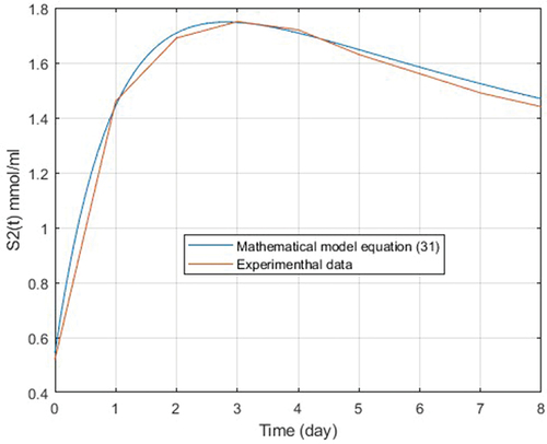
Figure 1. Experimental data of S₂ concentration (Table 3), (red color) and experimental mathematical model of S₂ (blue color).

(30) $S_2\left(\mathit{s}\right)=\frac{0.53002\left(\mathit{s}+0.0576427\right)\left(\mathit{s}+3.81635\right)}{\mathit{s}\left(\mathit{s}+1.00317\right)\left(\mathit{s}+0.11683\right)}$(30)

Hence, a mathematical model of the behavior of $S_2\left(\mathit{t}\right)$ is obtained as shown in Eq. (31)(31) $\widehat{S_2}\left(\mathit{t}\right)=0.99481221-1.58553\ast e^{-1.00317\mathit{t}}+1.12072\ast e^{-0.11683\mathit{t}}$(31) :

(31) $\widehat{S_2}\left(\mathit{t}\right)=0.99481221-1.58553\ast e^{-1.00317\mathit{t}}+1.12072\ast e^{-0.11683\mathit{t}}$(31)

The following figure (Figure 1) shows the comparison of discrete S₂(t) (experimental data) with the mathematical model obtained by regression Eq. (31)(31) $\widehat{S_2}\left(\mathit{t}\right)=0.99481221-1.58553\ast e^{-1.00317\mathit{t}}+1.12072\ast e^{-0.11683\mathit{t}}$(31) . With this method, a RMSE error found between their pointswas only 0.4%.

Theoretical model of $S_2\left(\mathit{t}\right)$

The AM2 model expressed through the ordinary differential equations system described in Eqs. (1)(1) $\frac{d{S}_1}{\mathit{dt}}=\mathit{D}\left(S_{1\mathit{in}}-S_1\right)-k_1{\mu }_1\left(S_1\right)X_1$(1) to (7(7) $q_M=k_6{\mu }_2\left(S_2\right)X_2$(7) ), is solved using the classical fourth-order Runge-Kutta numerical method, from which the behavior curve of the variable $S_2\left(\mathit{t}\right)$, using the calculated parameters k₂ and k₃ and the parameters k₁, k₄, k₅ and k₆ obtained by (Draa et al. 2018), the results are shown in Figure 2.

Figure 2. VFA concentration curve, using the parameters k₂ and k₃, generated by the theoretical model of S₂(t).

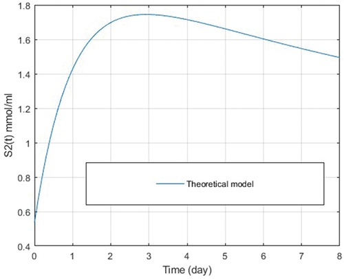
To build the theoretical curve using the Runge-Kutta numerical method for $S_2\left(\mathit{t}\right)$, successive calculations are made for the value of $S_2\left(\mathit{t}\right)$ at the instant following the current one $\left(y_{\mathit{i}+1}\right)$ starting from the current value $y_i$, to estimate the next value of VFA concentration $\left(y_{\mathit{i}+1}\right)$ . The algorithm used for the iteration procedure proposed by the classical fourth-order Runge-Kutta method implements Eq. (32)(32) $y_{\mathit{i}+1}=y_i+\frac{1}{6}\left(A_1+2A_2+2A_3+A_4\right)\mathit{h}$(32) .

(32) $y_{\mathit{i}+1}=y_i+\frac{1}{6}\left(A_1+2A_2+2A_3+A_4\right)\mathit{h}$(32)

where $\mathit{h}$ is the interval between $\left(\mathit{i}\right)\mathit{and}(\mathit{i}+1$) and $A_1$ to $A_4$ are functions calculated from Eqs. (33)(33) $A_1=\mathit{f}\left(x_i,y_i\right)$(33) to (36(36) $A_4=\mathit{f}\left(x_i+\mathit{h},y_i+A_3\mathit{h}\right)$(36) ).

(33) $A_1=\mathit{f}\left(x_i,y_i\right)$(33)

(34) $A_2=\mathit{f}\left(x_i+\frac{1}{2}\mathit{h},y_i+\frac{1}{2}{A}_1\mathit{h}\right)$(34)

(35) $A_3=\mathit{f}\left(x_i+\frac{1}{2}\mathit{h},y_i+\frac{1}{2}{A}_2\mathit{h}\right)$(35)

(36) $A_4=\mathit{f}\left(x_i+\mathit{h},y_i+A_3\mathit{h}\right)$(36)

Validation

To get the best approximation, it is evaluated with a sampling interval h = 0.02. With the above, it can be stated that the model obtained from Eq. (31)(31) $\widehat{S_2}\left(\mathit{t}\right)=0.99481221-1.58553\ast e^{-1.00317\mathit{t}}+1.12072\ast e^{-0.11683\mathit{t}}$(31) can be considered valid to represent experimental S₂(t) and compare it with theoretical S₂(t), the latter evaluated by numerical methods (Runge-Kutta) from k₂ y k₃ the AM2 model (Figure 3). The curve is parameterized by scaling to the maximum value of S₂(t) and an offset of 0.5 to adjust theoretical values to real values of the process.

Figure 3. Behavior of theoretical model S₂(t) (blue color) and experimental model S₂(t), (red color).

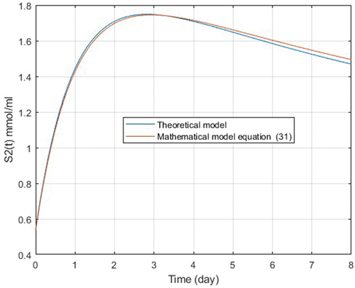
The error between the curves of the experimental and theoretical S2(t) model was calculated, with k = 42 values, 34 equidistant and 8 measured values. An error of 1.98% was found, which suggests a valid theoretical value of S₂(t), indirectly validating the calculated value of the parameters k₂ and k₃.

The results in Table 3 present a second-order exponential behavior. The mathematical model was obtained to compare the values obtained experimentally with the theoretical values within the 8-day time interval. The data in Figure 1 from the mathematical model superimposed on the graph constructed from the discrete data obtained from the periodic measurement of VFA shows the reliability of the mathematical model obtained to describe the behavior of the VFA concentration during the experimental time. The maximum error that occurs between the two of them is e <0.4%.

The curve constructed from the mathematical model AM2 using numerical methods, including k₂ and k₃ calculated based on the experimental phase, presents the same behavior observed in the curve constructed from the real VFA data from the same reactor. With the information already tabulated and modeled, two VFA behavior curves are constructed, shown in Figure 3, when compared result in a maximum error of 1.98%. Considering both error, it is achieved a maximum error <2.47%, which allows us to conclude that the values k₂ and k₃ obtained with the proposed method is valid for those used in the observer model D presented in this paper.

The experimental data obtained from the concentration of VFA, S₂(t), measured in experiment 2 are presented in Table 3 and Figure 1. Figure 2 shows the curve obtained with the S₂(t) theoretical model obtained by solving the AM2 model with the estimated parameters k₂ and k₃ and using the fourth-order Runge-Kutta numerical method, and the graph in Figure 3. With this information, an error of the theoretical model of S₂(t) is less or equal to 1.98%. This error agrees with the validation using VFA concentration as a variable in the D estimator, which has as stability condition D_min<D<D_max (D_med ± 5%); this allows validating the parameters k₂ and k₃ calculated in Eqs. (26)(26) $k_3=6.138\frac{\mathrm{mmol}C{H}_4}{0.0894\mathit{g}\mathit{VFA}}=68.65\frac{\mathrm{mmol}C{H}_4}{\mathit{g}\mathit{VFA}}$(26) and (31(31) $\widehat{S_2}\left(\mathit{t}\right)=0.99481221-1.58553\ast e^{-1.00317\mathit{t}}+1.12072\ast e^{-0.11683\mathit{t}}$(31) ).

Conclusions

An experimental method is proposed to determine the values of performance and consumption parameters embedded in the AM2 model, in particular the obtaining and validation of the parametders k₂ and k₃ used for the dilution rate obserever from the AM2 model.

To validate the proposed method, an indirect validation technique is established, which obtains the evolution of the dynamic behavior of the concentration of volatile fatty acids, S₂, based on the parameters k₂ and k₃ found and copares it with the value of S₂ observed experimentally.

The experimental mathematical model results for VFA concentration showed an error of <0.4% with respect to the experimental data. An error of <1.98% was found between the theoretical model and the experimental mathematical model. Overall, a global error of <2.37% gives a reliability to the proposed method to determine k₂ and k₃.

The above allows algorithms to be generated that automate and incorporate adaptive control strategies that help stabilize, control, and optimize the AD process.

This method can be applied to evaluate and validate other parameters of the model that cannot be measured but depend on other measurable process variables.

Based on the above, future work can be carried out to develop adaptive control strategies for process stability. Control strategies can be worked on in the future that use the dilution rate as a control variable using VFA and D observers.

Acknowledgements

Authors acknowledge the financial support provided by Dirección General de Asuntos del Personal. Académico (DGAPA), Universidad Nacional Autónoma de México (UNAM), México under PAPIIT Project No. IA104023.

Authors acknowledge the financial support provided by Ministerio de Ciencia y Tecnología de Colombia (MINCIENCIAS), Through Bicentenary Scholarships of the project called “Training of High-level human capital in Doctorate for regional development”.

Authors acknowledge the collaboration of the Doctorate in Engineering of the District University (Universidad Distrital Francisco José de Caldas).

Disclosure statement

No potential conflict of interest was reported by the author(s).

Supplementary material

Supplemental data for this article can be accessed online at https://doi.org/10.1080/15567036.2024.2311326

Additional information

Funding

The work was supported by the Dirección General de Asuntos del Personal Académico, Universidad Nacional Autónoma de México [IA104023]; Ministerio de ciencia, técnologia e innovación [Acuerdo 05 de 2020].

Notes on contributors

Orlando Harker-Sanchez

Orlando Harker-Sanchez received his degree in Electronic Engineering from Universidad Distrital Francisco José de Caldas, Colombia, and holds a Master’s degree from Universidad de La Salle, Bogotá. He is currently pursuing a Ph.D. in Engineering with a specialization in Electrical and Electronic Engineering from Universidad Distrital. Orlando is also a lecturer at Universidad Distrital, where he teaches control systems and industrial instrumentation. He is an active researcher in the LIFAE group in Renewable Energies.

Adolfo A. Jaramillo

Adolfo A. Jaramillo Matta received his degree in Electronic Engineering and a Master’s degree from the Universidad del Valle in Cali, Colombia. Later, he graduated with a Master’s and a PhD in Electronic, Automatic, and Telecommunications Engineering from the Rovira i Virgili University in Spain. He is currently a professor in the field of Control Systems at the Universidad Distrital. His research interests mainly include mathematical modeling of dynamic systems, automatic control systems, alternative energy sources, and power quality.

Dulce María Arias

Dulce María Arias is a Biochemical Engineer who specializes in environmental biochemistry. She completed her studies at the National Technological Institute of Mexico and obtained her PhD in Environmental Engineering from the Polytechnical University of Catalonia (UPC), where she was a member of the Environmental Engineering and Microbiology group (GEMMA). Currently, she works as a full professor and researcher at the Institute for Renewable Energies-UNAM. Her current research focuses on water and wastewater management, waste recovery and valorization, microbial fuel cells, and microalgae/cyanobacteria biotechnology for bioenergy and bioproducts production.

References

- Abdelhani, C., and S. Samia 2022. Identification of the AM2HN model parameters in the context of organic matter recycling. 2022 19th IEEE International Multi-Conference on Systems, Signals and Devices, SSD 2022 367–72. 10.1109/SSD54932.2022.9955922.
- Acosta-Pavas, J. C., C. E. Robles-Rodríguez, J. Morchain, C. Dumas, A. Cockx, and C. A. Aceves-Lara. 2023. Dynamic modeling of biological methanation for different reactor configurations: An extension of the anaerobic digestion model No. 1. Fuel 344 (March):128106. doi:10.1016/j.fuel.2023.128106.
- APHA-AWWA-WPCF. 2017. Standard methods for the examination of water and wastewater. 23rd ed. Washington, DC: American Public Health Association.
- Arshad, M., A. R. Ansari, R. Qadir, M. H. Tahir, A. Nadeem, T. Mehmood, H. Alhumade, and N. Khan. 2022. Green electricity generation from biogas of cattle manure: An assessment of potential and feasibility in Pakistan. Frontiers in Energy Research 10 (August):1–10. doi:10.3389/fenrg.2022.911485.
- Bastin, G., and D. Dochain. 1991. Online estimation and adaptive control of bioreactors. Analytica Chimica Acta 243:324. doi:10.1016/s0003-2670(00)82585-4.
- Bolzonella, D., D. Bertasini, R. Lo Coco, M. Menini, F. Rizzioli, A. Zuliani, F. Battista, N. Frison, A. Jelic, and G. Pesante. 2023. Toward the Transition of Agricultural Anaerobic Digesters into Multiproduct Biorefineries. Processes 11 (2):415. doi:10.3390/pr11020415.
- Chorukova, E., V. Hubenov, Y., Gocheva, and I. Simeonov. 2022. Two-phase Anaerobic Digestion of Corn Steep Liquor in Pilot scale biogas plant with automatic control system with Simultaneous Hydrogen and methane production. Applied Sciences 12 (12):6274.
- Dekhici, B., B. Benyahia, B. Cherki, B. Dekhici, B. Benyahia, B. Cherki, and D. Mode. 2022. Dynamic mode decomposition with control for data-driven modeling of anaerobic digestion process to cite this version: HAL Id: Hal-03696038 dynamic mode decomposition with control for data-driven modeling of.
- Dittmer, C., J. Krümpel, and A. Lemmer. 2021. Modeling and simulation of biogas production in full scale with time series analysis. Microorganisms 9 (2):1–10. doi:10.3390/microorganisms9020324.
- Draa, K. C., H. Voos, M. Alma, and M. Darouach 2015. Linearizing control of biogas flow rate and quality. IEEE International Conference on Emerging Technologies and Factory Automation, ETFA 2015 (October 3): 1–4. 10.1109/ETFA.2015.7301556.
- Draa, K. C., H. Voos, M. Alma, A. Zemouche, K. C. Draa, H. Voos, M. Alma, A. Zemouche, and M. D. Observer. 2018. Observer-based trajectory tracking for anaerobic digestion process mohamed darouach to cite this version: HAL Id: Hal-01683627 observer-based trajectory tracking for anaerobic digestion process.
- DuBois, M., K. A. Gilles, J. K. Hamilton, P. A. Rebers, and F. Smith. 1956. Colorimetric method for determination of sugars and related substances. Analytica Chimica Acta 28 (3):350–56. doi:10.1021/ac60111a017.
- Ficara, E., S., Hassam, A., Allegrini, A., Leva, F., Malpei, and G. Ferretti. 2012. Anaerobic digestion models: a comparative study. IFAC Proceedings Volumes 45 (2):1052–57.
- Gavala, H. N., I. Angelidaki, and B. K. Ahring. 2003. Kinetics and modeling of anaerobic digestion process. Advances in Biochemical Engineering/biotechnology 81:57–93. doi:10.1007/3-540-45839-5_3.
- Hajji, A., M. Rhachi, M. Garoum, and N. Laaroussi 2016. The effects of pH, temperature and agitation on biogas production under mesophilic regime. 2016 3rd International Conference on Renewable Energies for Developing Countries, REDEC2016:1–4. 10.1109/REDEC.2016.7577510.
- Kabeyi, M. J. B., and O. A. Olanrewaju. 2022. Technologies for biogas to electricity conversion. Energy Reports 8:774–86. doi:10.1016/j.egyr.2022.11.007.
- Kalyuzhnyi, S. V., D. J. Batstone, V. A. Vavilin, S. G. Pavlostathis, H. Siegrist, W. T. M. Sanders, A. Rozzi, I. Angelidaki, and J. Keller. 2002. The IWA Anaerobic Digestion Model No 1 (ADM1). Water Science and Technology 45 (10):65–73. doi:10.2166/wst.2002.0292.
- Lara-Cisneros, G., and D. Dochain 2018. Online estimation of the VFA concentration in anaerobic digestion processes based on a super-twisting observer. 2018 5th International Conference on Control, Decision and Information Technologies, CoDIT 2018:545–49. 10.1109/CoDIT.2018.8394870.
- Liu, X., A. Coutu, S. Mottelet, A. Pauss, and T. Ribeiro. 2023. Overview of numerical simulation of solid-state anaerobic digestion considering hydrodynamic behaviors, phenomena of transfer, biochemical kinetics and statistical approaches. Energies 16 (3):1108. doi:https://doi.org/10.3390/en16031108.
- Manjusha, C., and B. S. Beevi. 2016. Mathematical modeling and simulation of anaerobic digestion of solid waste. Procedia Technology 24:654–60. doi:10.1016/j.protcy.2016.05.174.
- Méndez-Acosta, H. O., A. Campos-Rodríguez, V. González-Álvarez, J. P. García-Sandoval, R. Snell-Castro, and E. Latrille. 2016. A hybrid cascade control scheme for the VGA and COD regulation in two-stage anaerobic digestion processes. Bioresource Technology 218:1195–202. doi:10.1016/j.biortech.2016.07.076.
- Mo, R., W. Guo, D. Batstone, J. Makinia, and Y. Li. 2023. Modifications to the anaerobic digestion model no. 1 (ADM1) for enhanced understanding and application of the anaerobic treatment processes – a comprehensive review. Water Research 244 (May):120504. doi:10.1016/j.watres.2023.120504.
- Olatunji, K. O., D. M. Madyira, and O. Adeleke. 2023. Optimizing anaerobic co-digestion of xyris capensis and duck waste using neuro-fuzzy model and response surface methodology. Fuel 354 (June):129334. doi:10.1016/j.fuel.2023.129334.
- Pan, N., H., Wang, Y., Tian, E., Chorukova, I., Simeonov, and N. Christov. 2022. Comparison study of dynamic models for One-stage and two-stage anaerobic digestion processes. IFAC-Papersonline 55 (7):667–72. doi:10.1016/j.ifacol.2022.07.520.
- Rodríguez-Mata, A. E., E. Gómez-Vidal, C. A. Lucho-Constantino, J. A. Medrano-Hermosillo, R. Baray-Arana, and P. A. López-Pérez. 2023. State estimation in a biodigester via nonlinear logistic observer: Theoretical and simulation approach. Processes 11 (4):1–17. doi:10.3390/pr11041234.
- Salamanca-Valdivia, M. A., L. Cardenas-Herrera, J. E. Barreda-Del-Carpio, G. M. Moscoso-Apaza, R. E. Garate-De-Davila, and C. A. Munive-Talavera 2021. Production of biogas in a dry anaerobic digestion reactor of residues generated in the processing of sheep and alpaca wool. 10th IEEE International Conference on Renewable Energy Research and Applications, ICRERA 2021:152–54. 10.1109/ICRERA52334.2021.9598668.
- Salgado, J. A. A. (2019). Modeling and simulation of biogas production based on anaerobic digestion of energy crops and manure. Master Thesis.
- Stinga, F., E., Petre, and M. Marian. 2017. Multiple predictive control of an anaerobic digestion process of microalgae. In 21st International Conference on System Theory, Control and Computing (ICSTCC). IEEE. 384–89. doi:10.1109/ICSTCC.2017.8107064.
- Sun, H., Z. Yang, G. Liu, Y. Zhang, Y. W. Tong, and W. Wang. 2023. Double-edged effect of tar on anaerobic digestion: Equivalent method and modeling investigation. Energy 277 (May):127738. doi:10.1016/j.energy.2023.127738.
- Tawai, A., M. Sriariyanun, and P. L. Gentili. 2022. Nonlinear Optimization-Based Robust Control Approach for a Two-Stage Anaerobic Digestion Process. Journal of Chemistry 2022:1–18. doi:10.1155/2022/8966350.