Population response of pelagic fishes (ciscoes, Coregonus spp.) to rapidly accelerated eutrophication of an originally oligotrophic deep lake

Figures & data

Figure 1: Bathymetric map of Lake Stechlin. Black lines indicate the 20 hydroacoustic transects surveyed annually. The four dashed brown lines indicate the approximate location of the midwater trawl transects.

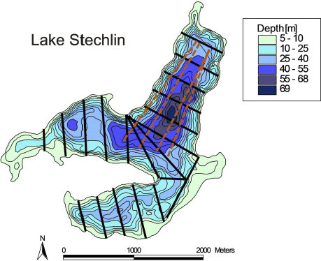
Figure 2: Panel a) Temporal trends of annual averages in total phosphorus concentration (mg m^-3), b) water temperature (°C) at 5 m and 40 m depths, respectively, c) Secchi depth (m), and d) oxygen concentrations (mg L^-1) at 5 m and 40 m depths, respectively, in Lake Stechlin between 2008 and 2021. Solid lines reflect significant (P < 0.05) linear regressions of the variable over time.

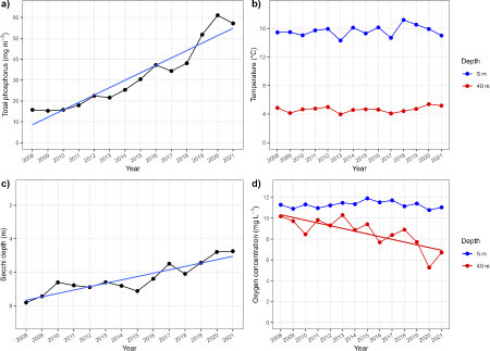
Table 1: Summary of results of linear regressions on temporal trends in abiotic and biotic variables from Lake Stechlin in the years 2008 to 2021. Values are annual averages from high-resolution measurements obtained once or twice per month (abiotic variables, chl a, zooplankton) or from annual fishing surveys conducted in June each year. Hydroacoustic daytime surveys were missing in 2014, while trawl data were missing in 2016. Abbreviations are used in figures showing cross-correlations between variables. wm = wet mass, dm = dry mass.

Dependent variable	Abbreviation	Unit	No. years	Slope	Mult. R²	t-value	P
Total phosphorus concentration	TP	mg m^-3	14	0.254	0.903	10.6	<0.0001
Secchi depth	Secchi	m	14	-4.03	0.811	-7.17	<0.0001
Water temperature 5 m	Temp5	°C	14	1.42	0.067	0.93	0.37
Water temperature 40 m	Temp40	°C	14	3.18	0.093	1.11	0.29
Oxygen concentration 5 m	Oxygen5	mg L^-1	14	0.172	0.0001	0.04	0.97
Oxygen concentration 40 m	Oxygen40	mg L^-1	14	-2.31	0.604	-4.28	0.0011
Fish abundance hydroacoustics	FishAbu	ind. 1000 m^-3	14	-0.046	0.022	-0.52	0.61
Fish biomass hydroacoustics	FishBM	kg wm ha^-1	14	0.038	0.149	1.45	0.17
Fish size hydroacoustics	FishSize	g wm	14	0.458	0.313	2.34	0.038
Fish depth day hydroacoustics		m	13	-0.179	0.050	-0.8	0.44
Fish depth night hydroacoustics		m	14	-0.589	0.193	-1.69	0.12
Fish migration amplitude hydroacoustics		m	13	-0.061	0.007	-0.28	0.78
Fish abundance trawl		ind. 1000 m^-3	13	0.142	0.059	0.83	0.42
Fish biomass trawl		g wm 1000 m^-3	13	0.010	0.348	2.42	0.034
Fish size trawl		g wm	13	0.211	0.234	1.83	0.094
Proportion Fontane cisco biomass trawl		%	13	-27.7	0.224	-1.78	0.10
Chlorophyll a	Chl a	mg m^-3	14	2.52	0.268	2.1	0.058
Zooplankton biomass Epilimnion	ZPEpiTot	mg dm m^-3	14	0.217	0.304	2.29	0.041
Zooplankton biomass fish prey Epilimnion	ZPEpiPrey	mg dm m^-3	14	0.249	0.339	2.48	0.029
Zooplankton biomass Hypolimnion	ZPHypoTot	mg dm m^-3	14	0.924	0.819	7.37	<0.0001
Zooplankton biomass fish prey Hypolimnion	ZPHypoPrey	mg dm m^-3	14	2.42	0.748	5.97	<0.0001

Figure 3: Panel a) Temporal trends of volumetric fish abundance (individuals 1000 m^-3), b) areal fish biomass (kg wet mass ha^-1), c) average individual fish size (g wet mass), d) average population depth during daytime (m), e) average population depth during nighttime (m) and f) average migration amplitude (m) in Lake Stechlin between 2008 and 2021. Dots represent ping-weighted averages (± 95% confidence intervals) of 20 transects (abundance, biomass and population depths), or geometric mean individual fish sizes (± 95% confidence intervals), as calculated from single echo detections from all transects combined. The blue line reflects significant (P < 0.05) linear regression of the variable over time.

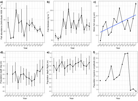
Figure 4: Panel a) Temporal trends of volumetric fish abundance (individuals 1000 m^-3), b) volumetric fish biomass (g wet mass 1000 m^-3), c) mean fish size (g wet mass) and d) proportion of Fontane cisco (Coregonus fontanae) biomass in total trawl catches in Lake Stechlin between 2008 and 2021. Data were obtained by midwater trawl surveys in four water depths in June (2008-2019, survey missed in 2016) or November (2020 and 2021). Dots represent arithmetic averages (± 95% confidence intervals) of four pelagic midwater trawl hauls (abundance, biomass). Mean fish size was calculated as average biomass divided by average abundance. Blue solid line reflects significant (P < 0.05) linear regression of the variable over time, while dotted blue lines reflect linear regressions with P<=0.10.

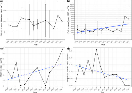
Figure 5: Panel a) Temporal trends of chlorophyll a concentration (mg m^-3), and b) zooplankton volumetric biomass (mg dry mass m^-3) in Lake Stechlin between 2008 and 2021. Chlorophyll a data reflect samples mixed from 0-5 m (May to October) or 0-10 m (November to April) depths, and averaged annually. Zooplankton were sampled in epilimnetic (0-22 m) and hypolimnetic layers (22-65 m), and expressed as either total biomass of all taxa, or biomass of taxa known to be prey for coregonid fishes (cladocerans, juvenile copepods). Data were obtained by one or two samples per month per year, and averaged to annual values. Solid lines reflect significant (P < 0.05) linear regressions, dashed line reflect a strong temporal trend (P ≤ 0.10) of the variable over time.

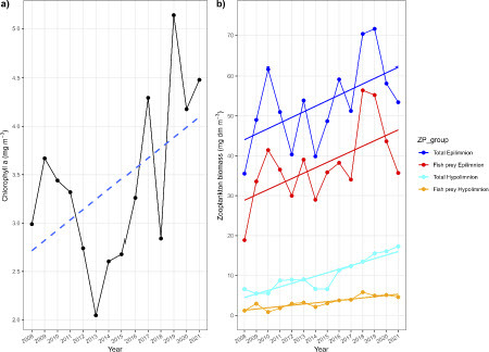
Figure 6: Bivariate Pearson correlation matrix among 14 annually averaged variables (for abbreviations, see Table 1) from Lake Stechlin between 2008 and 2021. Fish variables were obtained by nighttime hydroacoustics. Values are correlation coefficients for pairs of variables. Strong trends (P ≤ 0.10 for n = 14 years) in positive correlations are indicated by blue circles, while strong trends in negative correlations are indicated by red circles. Circle size and color intensity scale with interaction strengths.

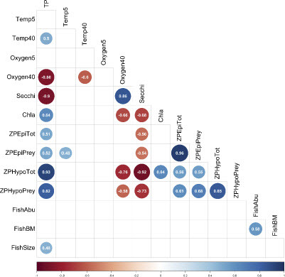
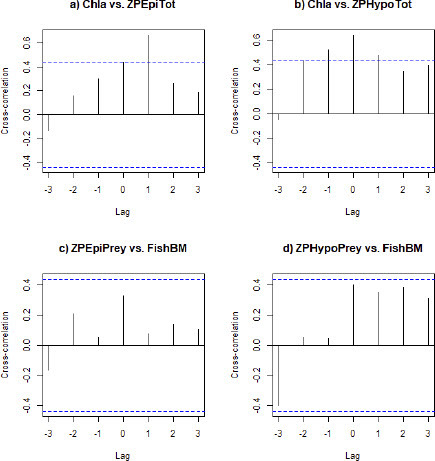
Figure 7: Cross-correlations with time lags up to three years between chlorophyll a concentration and zooplankton biomass in the epilimnion (a), chlorophyll a concentration and zooplankton biomass in the hypolimnion (b), zooplankton biomass of epilimnetic fish prey groups and fish biomass (c) and zooplankton biomass of hypolimnetic fish prey groups and fish biomass (d). Horizontal dashed blue lines represent 90% confidence intervals.