Two decades of fire activity over the PEEX domain: a look from space, with contribution from models and ground-based measurements

Figures & data

Figure 1. PEEX domain, selected areas, and selected locations. Background – land types map (https://lpdaac.usgs.gov/products/mcd12c1v006/, last access 25.08.2023). Coordinates of the selected areas are provided in the supplement (Table S2).

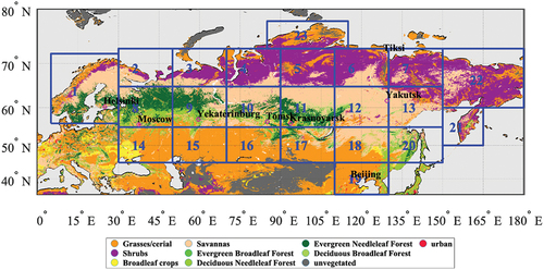
Figure 2. Cumulative FRP (MW, 10⁶) over the summer season (May to August) over the PEEX domain for 2002–2022 obtained from the MODIS instrument.

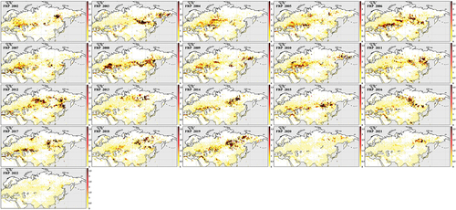
Figure 3. For AOD, HCHO, CO, and NO₂ (panels left-right), background monthly values (May to August, panels top-down) obtained from 2002–2022 (for AOD and CO; 2005–2020 for HCHO; 2005–2022 for NO₂) monthly products.

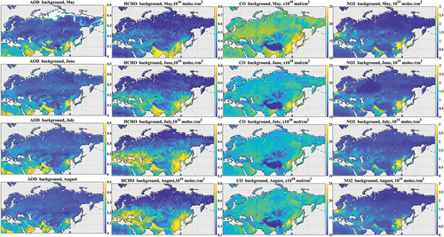
Figure 4. For July 2002–2022, mean actual values (upper panel) for lnFRP (a), T (b), P (c), SM (d), AOD (e), HCHO (f), CO (g), and NO₂ (h) and mean monthly values (lower panel) for the same variables after removal of the background values (except for lnFRP, which remains unchanged).

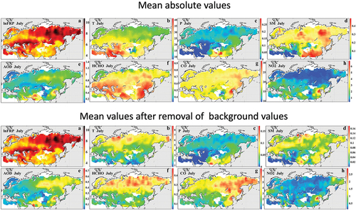
Figure 5. Mean lnFRP for July 2002–2022. (a) Spatial distribution of the correlation coefficients (p-value < 0.05) between lnFRP and temperature, T (b), precipitation, P (c), soil moisture, SM (d), AOD (e), HCHO (f), CO (g), and NO₂ (h) for July 2002–2022.

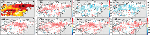
Table 1. For July, for the whole PEEX domain and different land types, the mean statistically significant (p < 0.05) correlation coefficients between lnFRP and T, P, SM, AOD, CO, HCHO, and NO₂.

	T	P	SM	AOD	CO	HCHO	NO2
PEEX domain	0.28	−0.28	−0.30	0.27	0.29	0.33	0.29
Land type
grass	0.27	−0.25	−0.25	0.12	0.25	0.27	0.25
shrubs	0.38	−0.32	−0.36	0.28	0.21	0.30	0.35
broadleaf crops	0.29	−0.26	−0.25	0.20	0.21	0.25	0.38
forest	0.24	−0.29	−0.33	0.32	0.34	0.34	0.22
savannas	0.27	−0.28	−0.31	0.32	0.30	0.36	0.33

Figure 6. For May 2006 (intense cropland fires in southern Russia and Kazakhstan), satellite lnFRP and ERA5 anomalies of meteorological parameters (T, P, and SM), satellite AOD and gas emission (HCHO, CO, NO₂) calculated with respect to median (2005–2017) values.

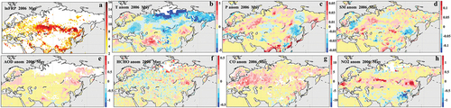
Figure 7. For August 2013 (intense fires in Siberia and eastern Europe), same as Figure 6.

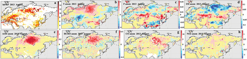
Figure 8. For August 2013, scatter plots of lnFC versus lnFC(a), meteorological parameters (temperature, (b); precipitation, (c); soil moisture, (d)), AOD (e), HCHO (f), CO (g), and NO₂ (h) with colour showing the latitude dependence (colourbar, latitudinal zones). Red dots correspond to the Sakha (Russia) area; magenta dots correspond to Jinan (China) area.

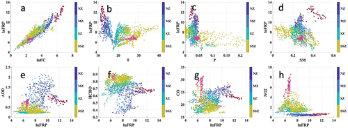
Figure 9. As Figure 8, scatter plot for anomalies.

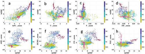
Table 2. For August 2013, correlation coefficients between different variables (Var1, Var2, actual values, and anomalies) for four zones (NZ, MZ, SZ, and SSZ) defined in Sect. 2. Statistically not significant values are replaced with *.

	Zones	NZ	MZ	SZ	SSZ	NZ	MZ	SZ	SSZ
Var1	Var2	for actual values				for anomalies
lnFC	lnFRP	0.88	0.91	0.85	0.56	0.35	0.79	−0.41	0.10
T	lnFRP	*	−0.62	0.42	0.40	−0.24	0.70	−0.44	−0.43
P	lnFRP	0.17	0.15	−0.62	−0.59	0.18	−0.24	−0.13	−0.10
SM	lnFRP	*	−0.43	−0.59	−0.66	*	−0.65	*	*
lnFRP	AOD	0.22	0.68	*	−0.44	0.24	0.69	0.10	0.15
lnFRP	HCHO	0.39	0.53	0.25	−0.49	0.26	0.58	0.11	0.25
lnFRP	CO	0.45	*	0.48	−0.08	0.34	0.73	*	−0.16
lnFRP	NO2	*	−0.60	−0.30	−0.41	0.35	0.57	−0.37	−0.11

Figure 10. Temporal and spatial distribution of FRP, temperature (T), precipitation (P), soil moisture (SM) (upper panel), and AOD, HCHO, CO, and NO₂ (lower panel) for July. The Y-axis shows the Areas (1–23) defined in Figure 1, while the X-axis shows the time (years). Vertical black dashed lines separate 5-year periods (e.g. 2006–2010 from 2011–2015), whereas horizontal green lines divide different latitudinal zones. Values for the variables are shown as a colorbar. The colorbar comprises of four primary colours (blue-green-magenta-orange, from low to high values). Each colour (e.g. blue) is divided into sub-classes of different intensities, increasing from lower to higher (inside sub-class) values.

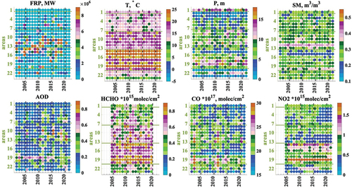
Figure 11. As Figure 10, for scaled anomalies.

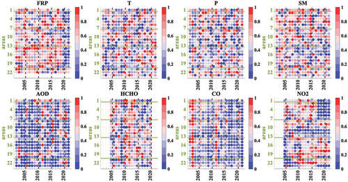
Table 3. For different domains, correlation coefficients between lnFRP and temperature (T), precipitation (P), soil moisture (SM), AOD, CO, HCHO, NO₂ for actual values (actual), anomalies (anom), relative anomalies (rel. anom), and scaled anomalies (scaled anom). Same after background values (BG) have been removed. Values are replaced with * if the corresponding p-value is >0.05.

		T	P	SM	AOD	CO	HCHO	NO2
Whole domain	actual	*	0.26	*	0.50	0.23	0.41	0.27
	BG removed	−0.39	0.23	0.34	0.47	0.41	0.30	*
	anom	−0.28	*	*	0.41	0.40	0.14	0.25
	rel.anom	0.16	−0.06	−0.10	0.19	0.21	0.21	0.16
	scaled anom	−0.17	−0.07	0.03	0.56	0.30	0.35	0.34
Zones:
SZ (45 º N–55º N)	actual	0.16	*	*	0.34	*	0.26	*
	BG removed	*	*	*	0.34	0.31	0.23	*
	anom	*	−0.27	*	0.31	0.27	0.23	*
	rel.anom	*	−0.27	*	0.33	0.29	0.26	*
	scaled anom	0.02	−0.28	−0.22	0.36	0.34	0.35	0.16
MZ (55 º N–65º N)	actual	0.34	*	−0.43	0.57	*	0.55	0.48
	BG removed	*	*	*	0.54	0.37	0.41	0.31
	anom	*	−0.31	−0.28	0.45	0.40	0.26	0.34
	rel.anom	*	−0.30	−0.28	0.49	0.40	0.30	0.39
	scaled anom	*	−0.31	−0.37	0.64	0.35	0.28	0.40
NZ (65 º N–73º N)	actual	0.73	0.42	−0.74	0.45	*	0.28	0.30
	BG removed	*	0.35	0.32	0.44	*	*	*
	anom	0.36	−0.33	−0.40	0.43	0.29	*	0.24
	rel.anom	*	−0.29	−0.38	0.43	0.26	*	*
	scaled anom	0.40	−0.23	−0.40	0.27	*	*	*
Areas:
Area 1, Scandinavia	actual	0.21	*	−0.48	*	*	0.37	0.15
	BG removed	0.32	−0.35	−0.30	*	0.28	0.31	0.15
	anom	0.32	−0.41	−0.51	*	0.35	0.32	*
	rel.anom	0.32	−0.43	−0.51	*	*	0.37	0.25
	scaled anom	0.46	−0.54	−0.54	*	*	0.47	*
Area 11, Central Siberia	actual	0.24	−0.47	−0.52	0.53	0.29	0.52	0.25
	BG removed	0.45	−0.49	−0.52	0.53	0.38	0.47	0.24
	anom	0.43	−0.56	−0.71	0.53	0.35	0.49	0.19
	rel.anom	0.29	−0.56	−0.71	0.54	0.35	0.58	*
	scaled anom	0.39	−0.43	−0.43	0.58	0.26	0.57	0.36
Area 19, Central China	actual	*	*	−0.45	*	*	*	*
	BG removed	0.26	−0.35	−0.37	*	*	0.65	0.26
	anom	0.24	−0.26	−0.34	0.21	0.02	0.60	0.23
	rel.anom	0.32	*	−0.30	*	*	0.43	*
	scaled anom	0.34	−0.29	−0.27	*	*	0.30	*

Figure 12. For central Siberia (Area 11), upper panel: scatterplots for lnFC, temperature (T), precipitation (P), and soil moisture (SM) monthly relative anomalies (x-axis) for years 2002–2022 and FRP relative anomalies (y-axis). Lower panel: scatterplots for different combinations of lnFRP relative anomalies (x-axis) and AOD, CO, HCHO, and NO₂ (y-axis) relative anomalies. Pearson correlation coefficient R is given on top of each panel; the p-value is provided. Percentages of points (from the total number of points) are shown in the “expected” quarters (e.g. for precipitation and soil moisture “expected” quarters are sector 90º–180º (T< 0or p < 0, and FRP > 0, coloured light yellow) and sector 270º–360º (T> 0 or p > 0, FRP < 0, coloured light orange); for other variables “expected” quarters are sector 0º–90º (anomalies are positive for both variables, coloured light red) and sector 180º–270º (anomalies are negative for both variables,coloured light blue)). The colour of the dots shows the month (see the legend).

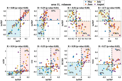
Figure 13. For central Siberia (Area 11), upper panel: scatterplots of scaled lnFC, T, P, SM (x-axis), and scaled FRP (y-axis). Lower panel: scatterplots scaled FRP (x-axis) and scaled AOD, CO, HCHO, and NO₂ (y-axis). The Pearson correlation coefficient R is shown on top of each panel. The color of each fit shows the month (see the legend).

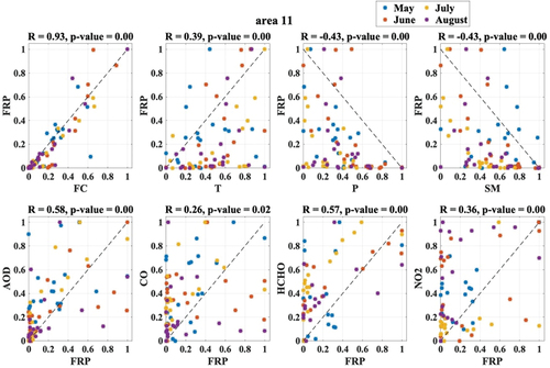
Figure 14. Decadal trends of FC, FRP, meteorological parameters, AOD, and atmospheric gases for the whole PEEX domain, zones NZ, MZ, and SZ, and Areas 1, 11, and 19. Units are as in Figure 10.

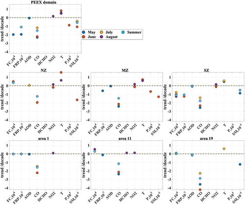
Figure 15. Top panel: AOD:CO ratios of monthly satellite data for pixels with FRP>0 (left); PM_2.5:CO from Akagi et al. (2011) (middle); PM_FRP:CO as in SILAM (right). Middle panel: same for AOD(or PM):HCHO. Lower panel: same for AOD(or PM):NO₂(or NO, NOx).

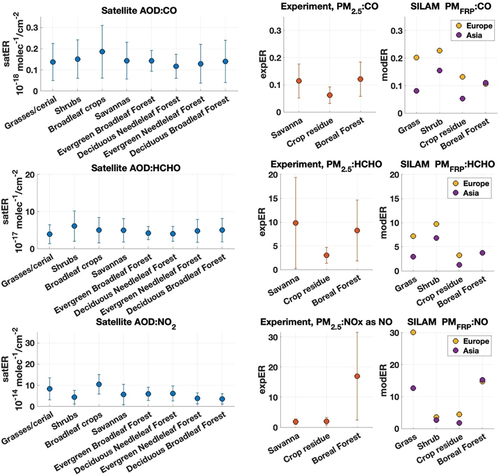
Figure 16. For three latitudinal zones (>65°N, 55°N–65°N, <55°N, columns left to right), satER for AOD:CO, AOD:HCHO, AOD:NO₂ (panels top-down).

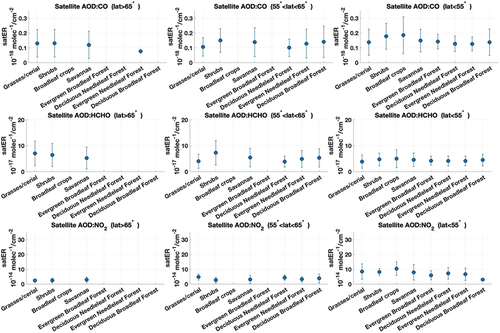
Figure 17. For different AOD ranges (all AOD, AOD ≤0.5, AOD ≥0.5, columns left to right), satER for AOD:CO, AOD:HCHO, AOD:NO₂ (panels top-down).

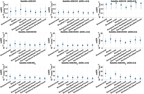
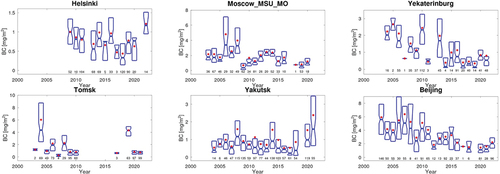
Figure 18. Boxplot of seasonal (May–August) columnar BC concentrations inferred from AERONET measurements for the following sites: Helsinki, Moscow, Yekaterinburg, Tomsk, Yakutsk, and Beijing. Boxplots give the seasonal medians (with 5^th/95^th percentiles) of BC concentrations, and red points provide the mean values in addition. The numbers below the boxes indicate the total number of measurements included in the seasonal means/medians in each year.

May, N. W., Bernays, N., Farley, R., Zhang, Q., & Jaffe, D. A. (2023). Intensive aerosol properties of boreal and regional biomass burning aerosol at Mt. Bachelor observatory: Larger and black carbon (BC)-dominant particles transported from Siberian wildfires. Atmospheric Chemistry & Physics, 23, 2747–2764. https://doi.org/10.5194/acp-23-2747-2023

 Web of Science ®Google Scholar

Yurganov, L. N., Rakitin, V., Dzhola, A., August, T., Fokeeva, E., George, M., Gorchakov, G., Grechko, E., Hannon, S., Karpov, A., Ott, L., Semutnikova, E., Shumsky, R., & Strow, L. (2011). Satellite- and ground-based CO total column observations over 2010 Russian fires: Accuracy of top-down estimates based on thermal IR satellite data. Atmospheric Chemistry & Physics, 11, 7925–7942. https://doi.org/10.5194/acp-11-7925-2011

 Web of Science ®Google Scholar

Akagi, S. K., Yokelson, R. J., Wiedinmyer, C., Alvarado, M. J., Reid, J. S., Karl, T., Crounse, J. D., & Wennberg, P. O. (2011). Emission factors for open and domestic biomass burning for use in atmospheric models. Atmospheric Chemistry & Physics, 11(9), 4039–4072. https://doi.org/10.5194/acp-11-4039-2011

 Web of Science ®Google Scholar

Data availability statement

Larisa Sogacheva (2023). Satellite-retrieved AOD, CO, HCHO, and NO₂ background over the PEEX domain [Data set]. Finnish Meteorological Institute. https://doi.org/10.23728/FMI-B2SHARE.003652E36B1B4FABA14283DE53C50B61