Time-first approach for land cover mapping using big Earth observation data time-series in a data cube – a case study from the Lake Geneva region (Switzerland)

Figures & data

Figure 1. Localization of the study area with a Sentinel-2 RGB (B04-B03-B02) composite showing the extent of the 31TGM tile together with the biogeographical zones covered.

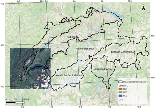
Figure 2. General workflow for the land cover map production using with the SITS package in R.

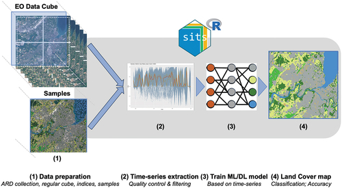
Table 1. SITS API main functions and their respective inputs and outputs (adapted from SITS book).

Step	API_function	Inputs	Output
1	sits_cube()	ARD image collection	Irregular data cube
	sits_regularize()	Irregular data cube	Regular data cube
	sits_apply()	Regular data cube	Regular data cube with new bands and indices
2	sits_get_data()	Data cube and sample locations	Time series
	sits_reduce_imabalance()	Time series samples	Balanced time-series
	sits_som_map()	Balanced time-series	Clean balanced time-series
	sits_kfold_validate()	Clean balanced time-series	Confusion matrix + F1 scores
3	sits_train()	Time series and ML method	ML classification model
4	sits_classify()	ML classification model and regular data cube	Probability cube
	sits_smooth()	Probability cube	Post-processed probability cube
	sits_label_classification()	Post-processed probability cube	Classified map
	sits_accuracy()	Classified map and validation samples	Accuracy assessment

Figure 3. Main functions of the SITS API and their respective interactions in the processing chain.

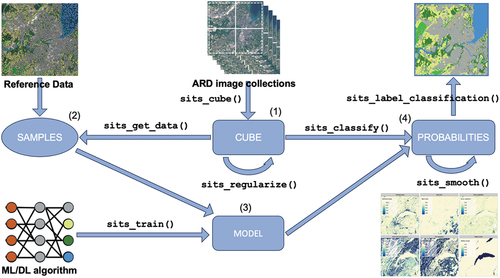
Figure 4. General implementation of the workflow in SITS. Satellite Analysis Ready Data are provided by the Swiss Data Cube (https://www.swissdatacube.ch); samples are gathered from the Arealstatistik dataset provided by the Federal Statistical Office.

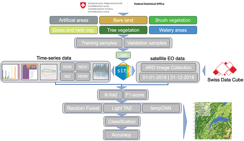
Figure 5. Aerial view over an area in Geneva (left); the sample points from the arealstatistik with the different classes of the NOLC04 Principal Domains (middle); and the translation in gridded land cover map (right).

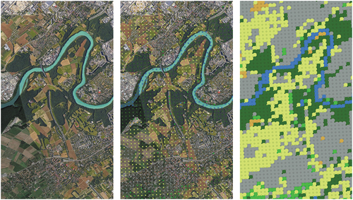
Table 2. Categories following the land cover NOLC04 classification separated in principal domains and basic categories.

Principal Domains	Basic Categories
10 – Artificial areas	15 – Lawns
	16 – Trees in artificial areas
20 – Grass and herb vegetation	21 – Gras and herb vegetation
30 – Brush vegetation	31 – Shrubs
	32 – Brush meadows
	33 – Short-stem fruit trees
	34 – Vines
	35 – Permanent garden plants and brush crops
40 – Tree vegetation	41 – Closed forest
	42 – Forest edges
	43 – Forest strips
	44 – Open forest
	45 – Brush forest
	46 – Linear woods
	47 – Cluster of trees
50 – Bare land	51 – Solid rock
	52 – Granular soil
	53 – Rocky areas
60 – Watery areas	61– Water
	62 – Glacier, perpetual snow
	63 – Wetlands
	64 – Reedy marshes

Figure 6. Patterns of the time-series for the six classes extracted using SITS. Each of six Principal Domains show different patterns that indicate potential good separability between the classes.

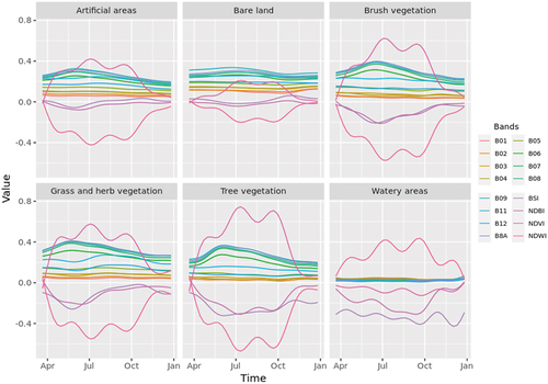
Figure 7. Confusion by cluster between the six different classes before (left) and after (right) pre-processing of the training samples.

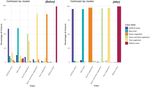
Table 3. Proportion of samples before and after the pre-processing of the training samples.

	Before pre-processing		After pre-processing
Label	Count	Proportion	Count	Proportion
Artificial areas	28884	0.10114862	1600	0.19314341
Bare land	7621	0.02668791	1150	0.13882183
Brush vegetation	9109	0.03189873	806	0.09729599
Grass and herb vegetation	120237	0.42105687	1600	0.19314341
Tree vegetation	86169	0.30175445	1600	0.19314341
Watery areas	33540	0.11745342	1528	0.18445196

Figure 8. Smoothed probabilities obtained for the tempCNN model and each land cover classes according to the NOLC04 nomenclature.

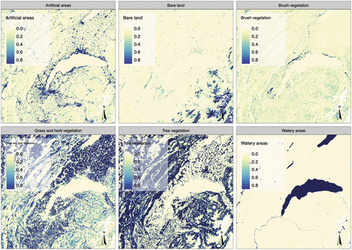
Figure 9. Final output of the classification obtained with the tempCNN model.

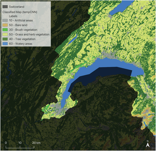
Table 4. Cross-validation showing accuracy, 95% Confidence Interval (CI), Kappa values, and F1-scores for the three tested methods: Random Forest (RF), lightweight temporal self-attention encoder (LTAE), and temporal convolutional neural network (tempCNN).

		RF	LTAE	tempCNN
Accuracy		0.9849	0.9703	0.9794
95% CI		(0.982, 0.9874)	(0.9664, 0.9739)	(0.9761, 0.9823)
Kappa		0.9817	0.964	0.975
F1-scores	Artificial areas	0.9812	0.9659	0.9697
	Grass and herb vegetation	0.9758	0.9528	0.9723
	Tree vegetation	0.9853	0.9798	0.9828
	Watery areas	0.9980	0.9951	0.9980
	Brush vegetation	0.9894	0.9655	0.9926
	Bare land	0.9817	0.9575	0.9634

Figure 10. Uncertainty of RF, LTAE, tempCNN models estimated through entropy estimation.

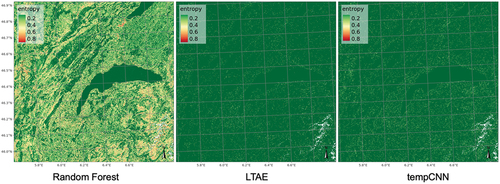
Table 5. Overall, users (UA) and producers (PA) accuracy for three models produced with a time-first approach and a comparison with the space-first approach.

	Space-first		Time-first
	RF		RF		LTAE		LTAE (tuned)		tempCNN		tempCNN (tuned)
Overall	0.82		0.85		0.83		0.86		0.86		0.90
	UA	PA	UA	PA	UA	PA	UA	PA	UA	PA	UA	PA
Artificial areas	0.65	0.61	0.67	0.63	0.75	0.54	0.69	0.65	0.69	0.65	0.75	0.67
Bare land	0.79	0.42	0.65	0.38	0.57	0.40	0.64	0.41	0.64	0.41	0.72	0.49
Brush vegetation	0.59	0.11	0.68	0.11	0.38	0.23	0.68	0.15	0.68	0.15	0.71	0.19
Grass and herb vegetation	0.82	0.82	0.87	0.87	0.86	0.83	0.88	0.89	0.88	0.89	0.91	0.89
Tree vegetation	0.83	0.85	0.85	0.95	0.82	0.95	0.86	0.95	0.86	0.95	0.87	0.97
Watery areas	0.96	0.90	0.99	0.90	0.99	0.89	0.99	0.90	0.99	0.90	0.99	0.90

Figure 11. Visual comparison of an aerial image (left) with Arealstatistik (middle) and the classified Sentinel-2 data with the tuned tempCNN model (right). The top view shows a larger area than the bottom view that corresponds to a zoom in the red square. Legend is the same as Figure 9.

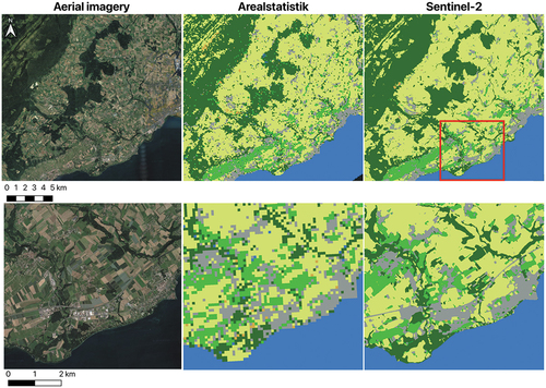
Table 6. Comparison of the proportions by class between the Arealstatistik and the classified Sentinel-2 data with the tuned tempCNN model.

	Arealstatistik			Sentinel-2
	Number (points)	Surface (km^2)	Proportion (%)	Number (pixels)	Surface (km^2)	Proportion (%)
Artificial areas	41588	415.88	10.14	4065402	406.54	9.91
Bare land	48250	482.5	11.77	4549149	454.92	11.09
Brush vegetation	12374	123.74	3.02	956667	95.67	2.33
Grass and herb vegetation	171829	1718.29	41.90	17766483	1776.65	43.32
Tree vegetation	13078	130.78	3.19	1081687	108.17	2.64
Watery areas	122992	1229.92	29.99	12589829	1258.98	30.70
Total	410111	4101.11	100.00	41009217	4100.92	100.00

Data availability statement

Sentinel-2 data that support the findings of this study are openly available at: https://doi.org/10.26037/yareta:zeg4u3pa5bcrfbph7mcsehorfm

Land Use Statistics, used as reference data are available at: https://www.bfs.admin.ch/bfs/de/home/statistiken/raum-umwelt/erhebungen/area.html

National Boundaries and Biogeographical regions can be obtained at: https://www.swisstopo.admin.ch/en/geodata/landscape/boundaries3d.html