The influence of channel morphology and hydraulic complexity on larval pallid sturgeon (Scaphirhynchus albus) drift and dispersal dynamics in the Fort Peck Segment, Upper Missouri River: insights from particle tracking simulations

Figures & data

Figure 1. Map showing the location of the study area (in red) within the segment of the Upper Missouri River Basin between Fort Peck Dam and Lake Sakakawea. The inset map shows the location of this area (in green) within the broader Missouri River Basin.

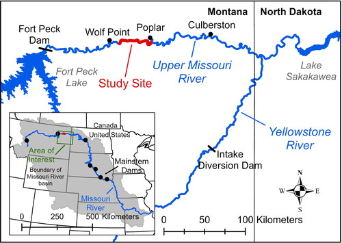
Figure 2. A Subset of the final channel-floodplain topographic surface. Topographic data are available in Call et al. (2024).

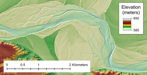
Figure 3. Map showing the locations of cross section measurements, 2019 larval drift experiment sampling stations, and the spatial extents of the 2018 and 2019 bathymetric surveys. Aerial imagery is from the USGS National Map (U.S. Geological Survey 2021).

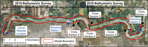
Table 1. Derived model parameters and the calibration RMSE for each of the three days that hydraulics measurements were taken.

Date	Discharge measured at Wolf Point gage	Downstream WSEL (m)	Roughness (Cd)	RMSE	LEV
06/10/2018	23,095 cfs (654 cms)	592.68	0.0051	0.0447	0.0469
09/07/2018	16,597 cfs (470 cms)	592.29	0.0057	0.0643	0.0343
07/01/2019	12,289 cfs (348 cms)	591.87	0.0054	0.0556	0.0259

Cfs, cubic feet per second; cms, cubic meters per second; WSEL, water surface elevation; m, meters; Cd, roughness coefficient; RMSE, root mean square error; LEV, lateral eddy viscosity.

Figure 4. Historic depth (a) and velocity (b) field measurements and corresponding fitted hydraulic geometry relations used to derive a representative power-law relationship for the LEV as Eq. (9)(9) $$\mathit{\text{LEV}}=0.01\left(0.096Q^{0.583}\right)\left(0.108Q^{0.358}\right)$$(9) (c).

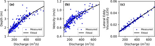
Figure 5. Water surface elevations derived by adjusting modeled values to better approximate measured values (a). Calibrated roughness values per discharge with Eq. (10)(10) $$\mathit{\text{Cd}}=\frac{n^{2}g}{h^{\raisebox{1ex}{$1$}\!\left/ \!\raisebox{-1ex}{$3$}\right.}}$$(10) plotted for manning’s n values of 0.028, 0.029, and 0.030 (b).

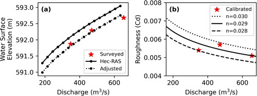
Figure 6. Comparisons of measured (red) and modeled (blue and black) depth-averaged velocities and depths for measurements made at cross-section 2 on June 10, 2018 (a and b, respectively), and September 9, 2018 (c and d, respectively). Solid blue lines represent values using hydrodynamics generated using the calibrated roughness parameter while the dashed black line represent hydrodynamics generated using the roughness parameter derived using Eq. (10)(10) $$\mathit{\text{Cd}}=\frac{n^{2}g}{h^{\raisebox{1ex}{$1$}\!\left/ \!\raisebox{-1ex}{$3$}\right.}}$$(10) .

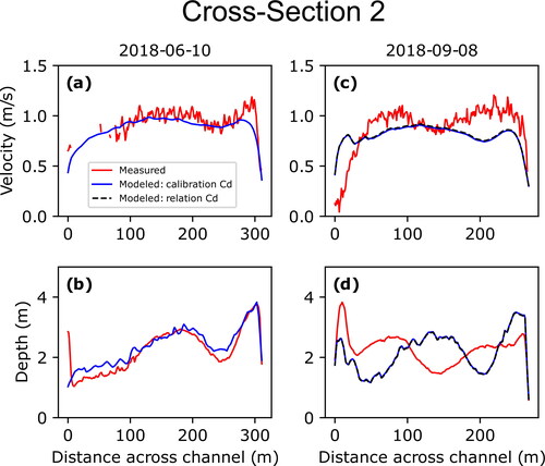
Figure 7. Comparisons of measured (red) and modeled (blue and black) depth-averaged velocities and depths for measurements made at cross-section 3 on June 10, 2018 (a and b, respectively), September 9, 2018 (c and d, respectively), and July 1, 2019 (e and f, respectively). Solid blue lines represent values using hydrodynamics generated using the calibrated roughness parameter while the dashed black line represent hydrodynamics generated using the roughness parameter derived using Eq. (10)(10) $$\mathit{\text{Cd}}=\frac{n^{2}g}{h^{\raisebox{1ex}{$1$}\!\left/ \!\raisebox{-1ex}{$3$}\right.}}$$(10) .

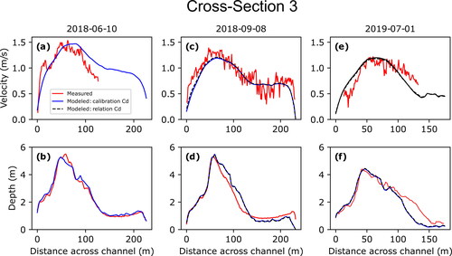
Figure 8. Comparisons of measured (red) and modeled (blue and black) depth-averaged velocities and depths for measurements made on July 1, 2019, at the larval drift experiment release site (a and b, respectively), sampling station 1 (c and d, respectively), and sampling station 2 (e and f, respectively). Solid blue lines represent values using hydrodynamics generated using the calibrated roughness parameter while the dashed black line represent hydrodynamics generated using the roughness parameter derived using Eq. (10)(10) $$\mathit{\text{Cd}}=\frac{n^{2}g}{h^{\raisebox{1ex}{$1$}\!\left/ \!\raisebox{-1ex}{$3$}\right.}}$$(10) .

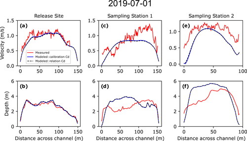
Figure 9. Map of the model reach showing the spatial extent of the upper reach (red) and the lower reach (blue) and their respective starting locations for Lagrangian particle tracking (LPT) simulations in addition to the channel centerline and reference points per kilometer from downstream to upstream used to identify general locations within the study reach.

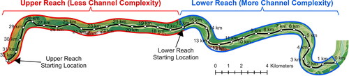
Figure 10. Comparisons of breakthrough curves from the 1-dimensional (1-D) model, Lagrangian particle tracking (LPT) simulations, and larval catch field data for 1-day-post-hatch (DPH) larvae at stations 1 and 2 (a and b, respectively) and 5-DPH larvae at stations 1 and 2 (c and d, respectively).

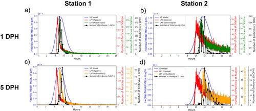
Figure 11. Comparison of median values of velocity, depth, and width (a, b, and c, respectively) and inter-quartile ranges (IQR) for velocity, depth, and width (d, e, and f, respectively) for the upper reach (red) and lower reach (blue).

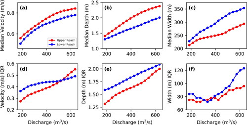
Figure 12. Comparison of median helix strength (a), number of emergent features (b), and total wetted perimeter (c) for the upper reach (red) and lower reach (blue).

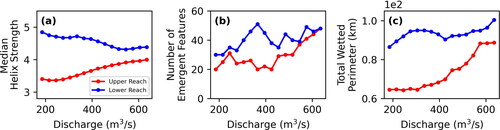
Figure 13. Each of the three vertical movement scenarios (passive is red, active75pct is blue, and active50pct is green) for the percent of particles retained for the upper and lower reaches (a and b, respectively), mean residence time for the upper and lower reaches (c and d, respectively), and mean transit time for the upper and lower reaches (e and f, respectively).

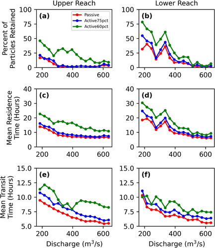
Figure 14. Median velocities (a and b) and depths (c and d) in the upper reach (a and c, respectively) and lower reach (b and d, respectively) for all particles (plotted as solid lines) and only those that exit the reach (plotted as dashed lines). Lines are colored according to the method of vertical movement (passive is red, active75pct is blue, active60pct is green). The black solid lines are the median velocities and depths calculated from hydrodynamic solutions for each reach.

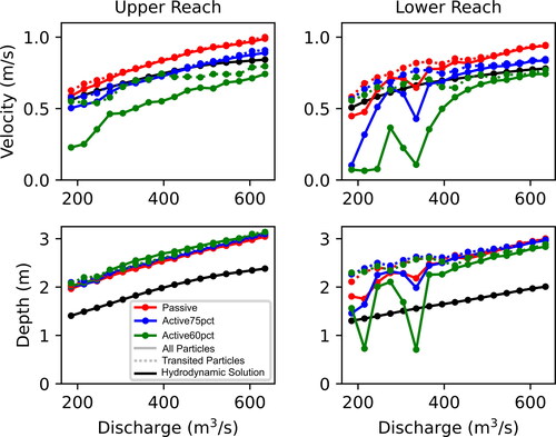
Figure A1. Location map showing the Upper Missouri River study area.

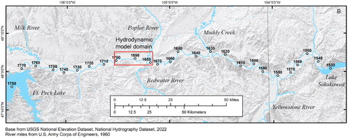
Figure A2. Longitudinal plot of geomorphic variables by 0.1 river mile, from upstream (left) to downstream (right). m, meters. Black vertical lines indicate the hydrodynamic model domain. Data source: Jacobson et al. (2023b).

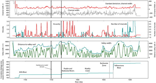
Figure B1.1. Comparisons of measured (red) and modelled (blue and black) depth-averaged velocities and depths for measurements made at cross-section 1 on June 10, 2018 (a and b, respectively), and July 1, 2019 (c and d, respectively). Solid blue lines represent values using hydrodynamics generated using the calibrated roughness parameter while the dashed black line represent hydrodynamics generated using the roughness parameter derived using Eq. (10)(10) $$\mathit{\text{Cd}}=\frac{n^{2}g}{h^{\raisebox{1ex}{$1$}\!\left/ \!\raisebox{-1ex}{$3$}\right.}}$$(10) .

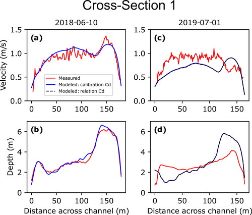
Figure B1.2. Comparisons of measured (red) and modelled (blue and black) depth-averaged velocities and depths for measurements made at cross-section 4 on June 10, 2018 (a and b, respectively), and September 9, 2018 (c and d, respectively). Solid blue lines represent values using hydrodynamics generated using the calibrated roughness parameter while the dashed black line represent hydrodynamics generated using the roughness parameter derived using Eq. (10)(10) $$\mathit{\text{Cd}}=\frac{n^{2}g}{h^{\raisebox{1ex}{$1$}\!\left/ \!\raisebox{-1ex}{$3$}\right.}}$$(10) .

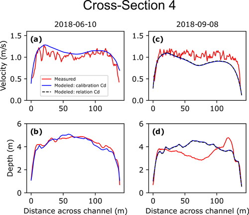
Figure B1.3. Comparisons of measured (red) and modelled (blue and black) depth-averaged velocities and depths for measurements made on June 10, 2018 (a and b, respectively), and September 8, 2018 (c and d, respectively) at cross-section 5. Solid blue lines represent values using hydrodynamics generated using the calibrated roughness parameter while the dashed black line represent hydrodynamics generated using the roughness parameter derived using Eq. (10)(10) $$\mathit{\text{Cd}}=\frac{n^{2}g}{h^{\raisebox{1ex}{$1$}\!\left/ \!\raisebox{-1ex}{$3$}\right.}}$$(10) .

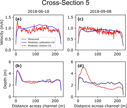
Figure B1.4. Comparisons of breakthrough curves from the 1-dimensional (1D) model, Lagrangian particle tracking (LPT) simulations, and larval catch field data for 1-day-post-hatch (DPH) larvae at stations 1 and 2 for LEVx0.5 (a and b, respectively), LEVx1 (c and d, respectively), and LEVx2 (e and f, respectively).

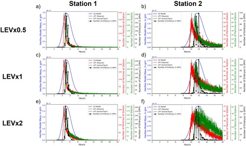
Figure B1.5. Comparisons of breakthrough curves from the 1-dimensional (1D) model, Lagrangian particle tracking (LPT) simulations, and larval catch field data for 5-days-post-hatch (DPH) larvae at stations 1 and 2 for LEVx0.5 (a and b, respectively), LEVx1 (c and d, respectively), and LEVx2 (e and f, respectively).

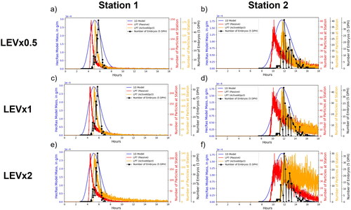
Figure B1.6. Comparison of percent particles retained for the upper reach (red) and lower reach (blue) for passive (first column), active75pct (second column), and active50pct (third column) vertical movement scenarios for LEVx0.5 (a, b, and c, respectively), LEVx1 (d, e, and f, respectively), and LEVx2 (g, h, and i, respectively).

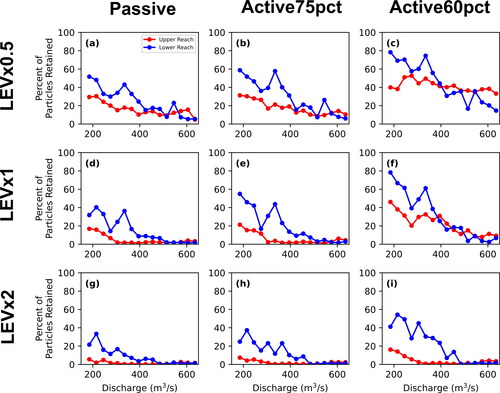
Figure B1.7. Comparison of mean residence time for the upper reach (red) and lower reach (blue) for passive (first column), active75pct (second column), and active50pct (third column) vertical movement scenarios for LEVx0.5 (a, b, and c, respectively), LEVx1 (d, e, and f, respectively), and LEVx2 (g, h, and i, respectively).

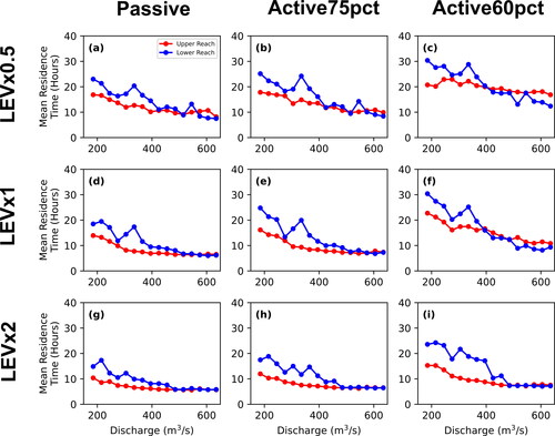
Figure B1.8. Comparison of mean transit time for the upper reach (red) and lower reach (blue) for passive (first column), active75pct (second column), and active50pct (third column) vertical movement scenarios for LEVx0.5 (a, b, and c, respectively), LEVx1 (d, e, and f, respectively), and LEVx2 (g, h, and i, respectively).

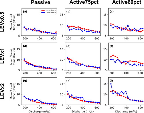
Table A1. Medians of geomorphic variables for the upper Missouri River, model domain, and upper and lower subsections.

	n	Average bankfull channel width, m	Standard deviation of channel width, m	Average channel sinuosity @ 3200 m	Maximum channel sinuosity @ 3200 m	Bankfull number of channels	Low-flow number of channels	Average valley width, m	Distance, channel to valley, m
Fort Peck Segment	2,448	323.0	105.8	1.25	4.91	1.17	NA	5,067	1,313
Model domain	224	359.3	106.1	1.15	1.58	1.02	2.0	6,237	1,380
Upper section	112	345.9	113.6	1.12	1.58	1.00	1.7	5,198	968
Lower section	112	369.9	100.2	1.18	1.47	1.04	2.3	7,054	1,703

Data are tabulated by 160 m sub reaches. Data source: Jacobson et al. (2023a). [NA, not applicable.].

Call BC, Erwin SO, Bulliner EA. 2024. Supporting files for particle tracking simulations of the Upper Missouri River near Wolf Point, MT. U.S. Geological Survey data. doi: 10.5066/P975PH68.

 Google Scholar

U.S. Geological Survey. 2021. USGS ImageryOnly Base Map. https://apps.nationalmap.gov/services/.

 Google Scholar

Jacobson RB, Elliott CM, Bulliner EA. 2023b. Geomorphic variables for classification of the Upper Missouri River, Montana and North Dakota. U.S. Geological Survey data. doi: 10.5066/P92HVKT3.

 Google Scholar

Jacobson RB, Elliott CM, Bulliner EA. 2023a. Geomorphic classification framework for assessing reproductive ecology of Scaphirhynchus albus (pallid sturgeon), Fort Peck segment, Upper Missouri River, Montana and North Dakota. Scientific Investigations Report 2023-5109. 15 pages. doi: 10.3133/sir20235109.

 Google Scholar

Data availability statement

All data used in this analysis are cited and available in sciencebase.gov (Call et al. 2024).