Connecting Land and Sea Vertical Datums: A Data Evaluation for Developing Australia’s AUSHYDROID Model

Abstract

Land and sea vertical datums have traditionally been separate reference levels, due to the different methodologies and observations used in their derivations. However, the need for a seamless connection of these datums has become important due to a wide range of applications in the coastal zone. This study evaluates existing methods, oceanographic and geodetic models and observations for the development of an operational model of coastal heights called AUSHYDROID. We use a complex study area in north west Australia to gain a new insight into how accurately the separation between the lowest astronomical tide (LAT) and a reference ellipsoid can be estimated from existing models, which could form the basis of a national AUSHYDROID model for Australia. Our results are the first attempt to use this combination of existing data in this location, suggesting that ellipsoidal heights of LAT can be estimated to an accuracy of ∼0.2 m at the coast, with the combination of DTU18MSS and FES2014b having the lowest RMS of 0.125 m. However, in some complex coastline areas such as bays and estuaries, the differences increase to >0.5 m so that additional tide gauge observations with GNSS levelling connections and improved models are needed in these regions.

Keywords:

• Tidal datum
• AUSHYDROID
• mean sea surface model
• lowest astronomical tide
• geoid
• ocean tide models
• marine chart
• coastal bathymetry

Introduction

The connection of heterogeneous datasets referenced to different land and sea vertical datums across the coastal boundary is fundamental to meet industrial and scientific requirements to support economic development, environmental and infrastructure protection and maritime and coastal safety (e.g. Slobbe et al. 2013a). This is particularly important for Australia with ∼85% of Australia’s population located on or near the coast (Ramm et al. 2017), and a heavy reliance on maritime trade and offshore resource development. In Australia, the AUSHYDROID working group has been established under the auspices of the Inter-Governmental Committee for Surveying and Mapping (ICSM) and leadership of the Australian Hydrographic Office (AHO) and tasked with developing an AUSHYDROID model that will facilitate the ocean-land vertical datum connection around Australia (see: https://www.icsm.gov.au/what-we-do/aushydroid). The term ‘hydroid’, which refers to the vertical separation between chart datum and a reference ellipsoid, was initially coined by Martin and Broadbent (2004), with the view that it is the ocean version of a geoid (hence AUSHYDROID as the maritime version of the gravimetric AUSGeoid; e.g. Featherstone et al. 2011), where the geoid height (N) is the vertical distance between the adopted geopotential surface and the chosen reference ellipsoid.

The motivation to develop an operational AUSHYDROID is due to the increasing national importance of Australia’s coastal and offshore regions for economic, security, maritime safety and environmental considerations. For example, understanding and estimating the vulnerability of residential and commercial property from rising sea levels, and the associated tidal surges depend on the accurate connection of land heights and sea heights (e.g. tide height and water depth). These are not currently defined in a single vertical datum where ocean modelling is related to tide gauges that may or may not be connected to the land height datum (cf. Figure 1). Moreover, many of the offshore datasets used are loosely connected to disparate vertical datums so that these cannot be directly compared with other data sets and land based vertical datums (cf. Iliffe et al. 2007). The benefits of connecting the land-sea vertical datums are that modelled and observed ocean heights can be directly related to land heights so that these risks, and their possible solutions, can be investigated and understood. The following examples highlight the diverse data sets and datums that abut, and often overlap at the coast:

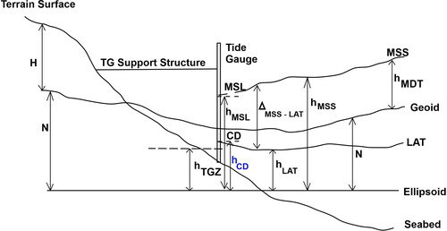
Figure 1. Reference datums/surfaces for land and sea in relation to each other: ocean’s time-mean dynamic topography (MDT), mean sea level (MSL; at the tide gauge) or mean sea surface (MSS; in the open ocean), lowest astronomical tide (LAT), tide gauge zero (TGZ), chart datum (CD), ellipsoidal height ($\mathrm{h}$), geoid-ellipsoid separation (N) and physical height (H) on the land vertical datum. Note that $\mathrm{h}=\mathrm{H}+\mathrm{N}$ on land, and $\mathrm{h}=\mathrm{\text{MDT}}+\mathrm{N}$ over the ocean.

1. Depths on maritime navigation charts are referenced to chart datum (CD) which is defined at a tidal height at specific port tide gauges.

2. Vertical land datums are historically based on a national levelling network constrained to historical mean sea level at specific tide gauges.

3. Modern Global Navigation Satellite Systems (GNSS) observations refer to an ellipsoid surface with a gravimetric geoid model used to transform (usually approximately) to the vertical datum.

In Australia, CD is defined as approximately lowest astronomical tide (LAT) under average atmospheric conditions fixed at a local tide gauge over a specified 20 year period (ICSM 2021). This provides a vertical reference for safe maritime navigation because the depths published on official nautical charts relate to the lowest tide at that specific tide gauge location under average conditions (cf. Slobbe et al. 2013a).

However, there are additional complexities in defining and connecting land-sea vertical datums because there are multiple variations and versions of each of the vertical datums depending on how, when and where they are defined (Wöppelmann, Zerbini, and Marcos 2006). For example, the Australian Height Datum (AHD; Roelse, Granger, and Graham 1971) was realised by the least squares adjustment of the national levelling network, fixed at mean sea level for 30 mainland tide gauges (observation period 1966–1968) and two Tasmanian tide gauges (observation period 1972). This has resulted in the north-south AHD slope with respect to an equipotential surface, which was shown by Featherstone and Filmer (2012) to approximately represent the ocean’s mean dynamic topography (MDT; Figure 1). A comparison of MDT estimates from 19 ocean and geodetic models by Filmer et al. (2018) demonstrated the different results from these models, which were dependent on the data and methods used to compute each model. Woodworth (2022) highlights the complexities of reconciling the vertical reference level for tide gauges at different locations. On the other hand, GNSS observations measured with respect to the surface of a reference ellipsoid provides a common reference to connect these data and disparate vertical datums and is now the basis for modern hydrographic surveys (e.g. Mills and Dodd 2014; Robin et al. 2016).

For a reference ellipsoid to be used as a common reference surface (Figure 1), GNSS observations need to be connected to tide gauges so as to relate the reference ellipsoid to the sea level observations (e.g. Bevis, Scherer, and Merrifield 2002; King 2014; Woodworth et al. 2017). Because GNSS observations are relatively recent compared to many of the tide gauge and other observations, the relation among these existing data and their respective vertical levels is often not well known, and in most historical cases can only ever be approximated. For example, sea level observations from tide gauges without a GNSS observation directly connected to the tide gauge zero (TGZ) will result in tide heights above an arbitrary datum, that cannot be related to other tide gauge records, maritime charts or sea surface heights derived from satellite radar altimetry. This causes difficulties in the numerous disciplines that require these connections; such as oceanography, hydrography, geodesy, flood forecasting, maritime navigation, coastal infrastructure management, etc.

While GNSS observations at the tide gauge will provide the ellipsoidal height ($\mathrm{h}$) of CD (${\mathrm{h}}_{\mathrm{\text{CD}}}$) at the specific tide gauge location (in the harbour) this value changes with distance from the tide gauge (Woodworth 2022). The key problem is that the ellipsoidal height of LAT (${\mathrm{h}}_{\mathrm{\text{LAT}}}$), which defines CD at the tide gauge, is spatially variable, thus changing in other areas of the harbour or bay, and the open sea, so that its value away from the defining tide gauge is uncertain. Considering this, the challenge is to relate all disparate vertical datums relative to CD (adopted from a specific time period of LAT) to a single reference surface, most conveniently nowadays a reference ellipsoid used by GNSS, so that the vertical difference relative to CD can be known (within a specified uncertainty) across all Australian coastal seas. Hence, the value ${\mathrm{h}}_{\mathrm{\text{CD}}}$ defines AUSHYDROID, to which all land and sea vertical datums are to be related. In reality, the objective is to estimate ${\mathrm{h}}_{\mathrm{\text{LAT}}}$ over the specified epoch, which is then adopted as ${\mathrm{h}}_{\mathrm{\text{CD}}}.$

Similar work has been undertaken in other national jurisdictions, each taking slightly different approaches to this problem, dependent on their measurement capability, data availability and their geographic situation. The key terms to determine ${\mathrm{h}}_{\mathrm{\text{CD}}}$ (refer to Figure 1) in seas away from the defining tide gauge are (1) ${\Delta }_{\mathit{\text{MSL}}‐\mathit{\text{LAT}}},$ which is the height difference between mean sea level (MSL) and LAT, determined at tide gauges, or ${\Delta }_{\mathit{\text{MSS}}‐\mathit{\text{LAT}}}$ which is the difference between mean sea surface (MSS) and LAT in the open ocean, (2) ${\mathrm{h}}_{\mathrm{\text{MSL}}}$ derived from tide gauges and GNSS at the coast, or ${\mathrm{h}}_{\mathrm{\text{MSS}}}$ over the open ocean derived from either satellite radar altimetry, or a combination of a geoid model (N) and an MDT model.

Sea level can be measured accurately at the tide gauge with MSL derived at this point location over a specified period of time, which is ideally 18.6 years so as to cover the full lunar nodal period (e.g. Woodworth 2012). The sea surface can be measured by satellite radar altimetry in the open ocean so that MSS can also be derived to a centimetre or two in the open ocean, but is less accurate close to the coast and in shallower waters (e.g. Vignudelli et al. 2019). This leaves a region or ‘gap’ between the open ocean and MSL at the tide gauge location on the coast where MSS is less accurately known. This is a key challenge, with Deng et al. (2002) previously recommending that satellite radar altimetry observations should be treated with caution within 22 km of the Australian coast, dependent on coastal topography contaminating altimetry waveforms, in addition to shallow water and bathymetry variations. However, there have been significant improvements in coastal altimetry results in recent years, with an example being X-Track reprocessed altimetry (Birol et al. 2017), which suggests improved results as close as 5 km from the coast (e.g. Seifi and Filmer 2023). Considering the demonstrated improvements in coastal altimetry, we will consider the coastal ‘gap’ where altimetry may be less reliable as ∼10 km for the purpose of this study. The results from this study will contribute further to our understanding of radar altimetry and the models using these data in these coastal regions.

Research in other national jurisdictions include the following: (1) The UK vertical offshore reference frame (VORF) where Iliffe et al. (2013) and Turner et al. (2013) incorporate information from satellite altimetry, tide and geoid models, tide gauges, and GNSS observations. Testing on the VORF project indicates accuracies of 0.10 m onshore and 0.15 m at offshore locations (Turner et al. 2013); (2) the Hydrographic Vertical Separation Surfaces (HyVSEPs) have been developed for Canadian tidal waters for the Continuous Vertical Datum for Canadian Waters (CVDCW; Robin et al. 2016); (3) the US VDATUM project (https://vdatum.noaa.gov/welcome.html) is able to transform between tidal and other land-based datums (Parker, Milbert, and Gill 2003); (4) the French approach in Bathyelli (Pineau-Guillou and Dorst 2013), differs in that it relies mostly on co-located GNSS and tide gauge observations along the coast, satellite radar altimetry offshore, and shipborne GNSS and water level surveys to fill in the gap areas. They did not use an MDT and geoid model to approximate the MSS in the open ocean as the Canadian, USA and UK approaches did; (5) the Netherlands (NEVREF) took a different approach again, where they used a geoid model and then estimated the vertical distance between LAT and the geoid (Slobbe et al. 2013a, 2013b, Slobbe et al. 2018). In this case, the important value is the LAT-geoid separation (${\Delta }_{\mathrm{\text{LAT}}‐\mathrm{\text{geoid}}}$) which was derived from a hydrodynamic and geoid model in the open ocean, and tide gauge records and a geoid model at the coast.

Progress has been made in Australia through the study of Keysers, Quadros, and Collier (2013, 2015) developing vertical coastal transformation software, but finding that there was insufficient tide gauge data at that stage to rigorously connect across the coastal boundary. On a local level, a high spatial and temporal resolution hydroid model was established around Port Hedland (northwest Australia) (Schlack and Hewitt 2015). This local example adjusted an existing single chart datum value based in the port, which was being applied uniformly along the (42 nautical mile) long shipping channel, to one that varied spatially in accordance with the diminishing offshore tidal range as measured by a series of tide gauges and GNSS receivers.

Our study presents a new approach for Australia, where we evaluate existing models and observations that could be used to develop AUSHYDROID in Australian coastal waters. We use state of the art ocean tide models (OTMs), geoid, MSS and MDT models combined with terrestrial tide gauge and GNSS observations in a challenging study area in north west Australia to assess the suitability of these data for building an operational AUSHYDROID. The aim is to determine the accuracy that could be achieved from these existing data as a step towards the design and development of AUSHYDROID. These results are significant as they show the characteristics of these models to realise ${\mathrm{h}}_{\mathrm{\text{LAT}}}$ for the first time in this coastal region of Australia.

Material and methods

There are a number of methods and data that can be used to connect land and sea vertical datums. Following from Figure 1, we break the quantities required down into a series of components related to experiences in international jurisdictions. Because ICSM (2021) defines CD as LAT over a defined period, we will consider ${\mathrm{h}}_{\mathrm{\text{LAT}}}$ as the key quantity for this study, which we treat as an approximation of ${\mathrm{h}}_{\mathrm{\text{CD}}}$ which can only be defined at the port tide gauge.

Methodology

To create an operational AUSHYDROID across the coastal region, a method is required to estimate ${\mathrm{h}}_{\mathrm{\text{LAT}}}$ over the open ocean that can be connected to tide gauges in harbours. This can be done using satellite radar altimetry-derived ocean heights of MSS above a defined ellipsoid (${\mathrm{h}}_{\mathrm{\text{MSS}}}$), and the modelled (absolute, that is, positive value) difference between the MSS and LAT (${\Delta }_{\mathrm{\text{MSS}}‐\mathrm{\text{LAT}}}$), which is computed from an OTM (e.g. Wöppelmann, Zerbini, and Marcos 2006). Alternatively, ${\mathrm{h}}_{\mathrm{\text{MSS}}}$ can be closely approximated by a model of MDT and the geoid so that ${\mathrm{h}}_{\mathrm{\text{MSS}}}\approx \mathrm{\text{MDT}}+\mathrm{N}$ (see Figure 1 for definitions), so that regardless of how ${\mathrm{h}}_{\mathrm{\text{MSS}}}$ is estimated: (1) $${\mathrm{h}}_{\mathrm{\text{LAT}}}\approx {\mathrm{h}}_{\mathrm{\text{MSS}}}-{\Delta }_{\mathrm{\text{MSS}}‐\mathrm{\text{LAT}}}$$(1)

To evaluate the available data and models, we derive ‘ground truth’ data (${\mathrm{h}}_{\mathrm{\text{LAT}}}$) using tide gauge observations at the coast in combination with GNSS levelling connections. Tide gauge ${\mathrm{h}}_{\mathrm{\text{LAT}}}$ is computed as (2) $${\mathrm{h}}_{\mathrm{\text{LAT}}}\approx {\mathrm{h}}_{\mathrm{\text{MSL}}}-{\Delta }_{\mathrm{\text{MSL}}‐\mathrm{\text{LAT}}}$$(2) where ${\Delta }_{\mathrm{\text{MSL}}‐\mathrm{\text{LAT}}}$ is the absolute (i.e. a positive value) vertical difference between MSL and LAT determined at the tide gauge. ${\mathrm{h}}_{\mathrm{\text{MSL}}}$ is the ellipsoidal height of MSL at the tide gauge computed as (cf., Filmer et al. 2018, Andersen et al. 2018a; Filmer and Featherstone 2012; Woodworth et al. 2012) (3) $${\mathrm{h}}_{\mathrm{\text{MSL}}}={\mathrm{h}}_{\mathrm{\text{TGBM}}}-\left(\Delta \mathrm{H}+\Delta \mathrm{N}\right)+{\mathrm{\text{MSL}}}_{\mathrm{\text{TGZ}}}$$(3) where ${\mathrm{h}}_{\mathrm{\text{TGBM}}}$ is the GNSS observed ellipsoidal height $\mathrm{h}$ at the tide gauge benchmark (TGBM), $\Delta \mathrm{H}$ is the physical height difference (levelling observations with height correction) between the TGBM and the tide gauge zero (TGZ), $\Delta \mathrm{N}$ is the geoid height difference between the TGBM and tide gauge location, which transforms the physical height difference to an ellipsoidal height difference, and ${\mathrm{\text{MSL}}}_{\mathrm{\text{TGZ}}}$ is MSL estimated from a time series of sea level observations relative to the TGZ. The notation $\mathrm{H}$ refers to a physical height (e.g. orthometric, or normal height) measured along the curved and torsioned plumb line, taking gravity potential into account and refers to the geoid, or quasigeoid respectively (e.g. Filmer, Featherstone, and Kuhn 2010). The quasigeoid and geoid coincide over the ocean, but diverge over land at higher elevations. The physical height $\mathrm{H}$ is different to $\mathrm{h},$ which is a GNSS-derived ellipsoidal height, measured along the ellipsoid normal and referred to a specific ellipsoid surface defined within an earth-centred geodetic datum (e.g. Jekeli 2000).

In this study, we refer to MSL as being the point-wise value estimated from sea level observations at a tide gauge over a period of time, whereas MSS is estimated from satellite radar altimetry observations over the open ocean related to the radar signal’s footprint over an area of the sea surface. Theoretically, they are both measuring the ocean surface when transformed to a common height datum, but are subject to different errors and noise due to the different measurement techniques. This is because MSL is an observation at a discrete point on the coast, but MSS from altimetry is the sea surface averaged over the area of the footprint. The challenge to estimate ${\mathrm{h}}_{\mathrm{\text{LAT}}}$ from models in Equation (1)(1) $${\mathrm{h}}_{\mathrm{\text{LAT}}}\approx {\mathrm{h}}_{\mathrm{\text{MSS}}}-{\Delta }_{\mathrm{\text{MSS}}‐\mathrm{\text{LAT}}}$$(1) is dependent on how accurately these models can represent MSS and ${\Delta }_{\mathrm{\text{MSS}}‐\mathrm{\text{LAT}}}$ at the coast and the adjacent ocean region where an operational AUSHYDROID is required.

Study area

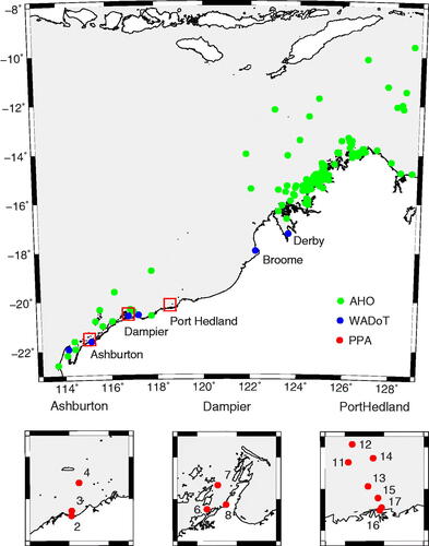
The study area in north west Australia along with the location of the tide gauges used are shown in Figure 2. The study area was selected because it is a challenging area with very large tidal ranges (up to 14 m; Griffin et al. 2021) along a complex coastline with bays, estuaries and harbours so that any problems with data quality and spatial or temporal frequency will be exacerbated and more easily identified. These data problems can then be addressed to facilitate the development of AUSHYDROID.

Figure 2. Locations of 10 WADoT tide gauges, 16 PPA tide gauges and 116 AHO tide gauges. The boxes (red in the online version) on the main plot at Ashburton, Dampier and Port Hedland relate to the inset boxes in the bottom row, showing the PPA tide gauges at these locations (numbered as per Table 1).

Tide gauge and GNSS observations

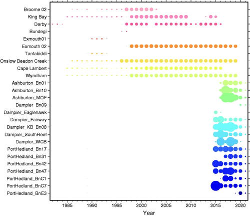
The tide gauge locations shown in Figure 2 are from three different sources; Pilbara Ports Authority (16 PPA; red circles), Western Australian Department of Transport (10 WADoT; blue circles), and the Australian Hydrographic Office (116 AHO; green circles). These tide gauge sets provide a total of 142 tide gauges, and are all quite diverse in their observation epoch, frequency and location. The epoch of the WADoT and PPA tide gauges are represented in Figure 3, with each circle representing the number of annual observations. The larger size the circle, the more observations for that year, indicating a change in the recording frequency. For instance, the WADoT tide gauge time series used a 15 min recording frequency up to ∼1995, but this was increased to 5 min after this time, resulting in more annual observations. The WADoT annual observations go back to 1982, but there are also gaps in some tide gauge records, which may be due to tide gauge malfunction, or removal of the tide gauge. The PPA tide gauges are all employed in the Ashburton, Dampier and Port Hedland maritime navigation areas, having been installed and operational from around 2015. The Port Hedland tide gauges have been used to upgrade the port datum for bulk shipping navigation, as described in Schlack and Hewitt (2015). On the other hand, all the AHO tide gauge recordings come from temporary short epoch installations (mostly between 30–60 days) that include recordings dating back to 1944, and as recently as 2020 in the HydroScheme Industry Partnership Program (HIPP; https://www.hydro.gov.au/NHP/hipp.htm).

Figure 3. Summary of 10 WADoT and 16 PPA tide gauge observations for the WA study area. The circle size increases with more observations for a given year (e.g. due to an increase in sample rate). Missing circles are where there are no observations – small circles may represent some data missing and/or a lower sampling rate for the given year. Locations for these sites are shown in Figure 2.

We use the software program UTide (Codiga 2011) to analyse the sea level observations from the tide gauge records to compute LAT and MSL. We have used the full tide gauge record to compute MSL, as per the time period illustrated in Figure 3. While it may be preferable to compute MSL from the tide gauges over the same time period as the MSS and MDT models (shown in Table 2), this is problematic due to the limited number of available tide gauges and their operating period. All of the WADoT tide gauge records used were at least 10 years long, with most covering the MSS/MDT/OTM periods, with the PPA tide gauge records mostly ∼5 years, but at the end, or after the MSS/MDT/OTM observation periods. To avoid truncating some tide gauge records to fit the model periods, we took a pragmatic approach and use the full tide gauge records for the MSL estimate. A discussion of these possible effects is in Section ‘Comment on compatibility of the models and observations’. We took a different approach to compute tide gauge ${\Delta }_{\mathrm{\text{MSL}}‐\mathrm{\text{LAT}}}.$ For consistency, we used the four main tidal constituents (M₂, S₂, K₁, O₁) and 5-year observation period 2006/01/01 to 2010/12/31 at WADoT tide gauges (where possible) and from each OTM. The PPA period was 2016/01/01 to 2020/12/31 (or as close as possible depending on the record) with the AHO period spanning their full 30–60 day record. Using only the four main tidal constituents enabled ${\Delta }_{\mathrm{\text{MSL}}‐\mathrm{\text{LAT}}}$ to be resolved at the 30–60 day AHO tide gauges.

Table 2. Details of the different models tested in this study to provide modelled ${\mathrm{h}}_{\mathrm{\text{LAT}}}$ to compare with tide gauge ${\mathrm{h}}_{\mathrm{\text{LAT}}}$ at the coast.

Model	Spatial res	Period	Source/availability (Download location)	References
MSS
CNES-CLS 2015 MSS	1’	1993–2012	Aviso+ at https://www.aviso.altimetry.fr/en/data/products/auxiliary-products/mss.html	Schaeffer et al. (2016a, 2016b)
DTU18 MSS	1’	1993–2017	DTU at ftp://ftp.spacecenter.dk	Andersen et al. (2018b, 2018c)
MDT
CNES-CLS18 MDT	7.5’	1993–2017	Aviso+ at https://www.aviso.altimetry.fr/en/data/products/auxiliary-products/mdt.html	Mulet et al. (2021)
DTU19MDT	1’	1993–2018	DTU, ftp://ftp.spacecenter.dk/pub/dtu19/mdt	Andersen and Knudsen (2009)
DTU15MDT	1’	1993–2014	DTU, ftp://ftp.spacecenter.dk/pub/dtu15/1_min	Andersen and Knudsen (2009)
Ocean tide
TPXO9v5	2’	1999–2010	Y. Erofeeva, pers. comm. (2021)	Egbert and Erofeeva (2002), Egbert, Erofeeva, and Ray (2010)
FES2014b	3.75’	1999–2014	Aviso+ at https://www.aviso.altimetry.fr/en/data/products/auxiliary-products/global-tide-fes.html	Lyard et al. (2021)
Geoid
AGQG 2017	1’	Variable	Curtin University	Featherstone et al. (2018)
EGM2008	5’	Variable	http://icgem.gfz-potsdam.de/home	Pavlis et al. (2012)
XGM2019e_2159	5’	Variable	http://icgem.gfz-potsdam.de/home	Zingerle et al. (2020)
EIGEN-6C4	5’	Variable	http://icgem.gfz-potsdam.de/home	Foerste et al. (2014)

Note that geoid models with 5’ spatial resolutions are computed from global gravity models to spherical harmonic degree/order 2190.

The tide gauge derived MSL and ${\Delta }_{\mathrm{\text{MSL}}‐\mathrm{\text{LAT}}}$ are treated as the ‘truth’ with the difference to these modelled values interpreted and analysed as ‘model errors’. We acknowledge that there are uncertainties in the tide gauge record and derived values, moreso in the short period (30 to 60 days) AHO tide gauges, where Turner et al. (2013) suggest differences of up to ±0.30 m between the short and long term MSL estimates may persist for up to a month. However, for multiyear tide gauge records as per those provided by WADoT and PPA, uncertainties in derived tide levels are considered negligible (no more than several cm) for the purpose of evaluating the models.

To compute Equation (3)(3) $${\mathrm{h}}_{\mathrm{\text{MSL}}}={\mathrm{h}}_{\mathrm{\text{TGBM}}}-\left(\Delta \mathrm{H}+\Delta \mathrm{N}\right)+{\mathrm{\text{MSL}}}_{\mathrm{\text{TGZ}}}$$(3) , all of the tide gauges will need to have GNSS observations with levelled height difference connections between the TGBM and the tide gauge. The three different data sources (WADoT, PPA and AHO) had these GNSS levelling connection data archived in different ways. GNSS heights for the 10 WADoT tide gauges in the WA study area were accessed through www.nationalmap.gov.au. The PPA provided GNSS heights of the TGZ at all 16 tide gauges which had been reprocessed in the Geocentric Datum of Australia 2020 (GDA2020) from more than 10 hours of observations (F. Schlack pers. comm., 2021). The AHO tide gauges had GNSS observations at recent tide gauge observations only, and these had to be manually searched and extracted from the provided 116 AHO data directories, and the connections recalculated.

A number of problems were identified with this archiving, so that only 10 AHO tide gauges were found to have suitable GNSS levelling connections for this study. This is only a small fraction of the 116 AHO tide gauges in the initial data set, however a combination of older tide gauges with no GNSS connections, possible blunders in observation, recording or archiving of GNSS, the levelling connection to the tide gauge, or the tide gauge record itself resulted in this small numbers of tide gauges being considered suitable for this study. Preliminary comparisons with these 10 tide gauges further identified some of these tide gauges as outliers, possibly also due to blunders in the GNSS or levelling observations, or incomplete or noisy tide gauge records. In addition, three WADoT tide gauges (Bundegai, Exmouth01 and Tantabiddi) had very short records so were removed, and three PPA tide gauges (DP Eaglehawk, DP BN09 and DP WCB) could also not be included due to short records or uncertainty over the ellipsoidal datum connection. The final data set used were observations from six WADoT, 13 PPA, and six AHO tide gauges, as shown in Table 1.

Table 1. Final 25 tide gauges used in this study for analysis. The tide gauges are ordered from west to east.

#	Tide gauge name	Latitude	Longitude	Observation period
1	Exmouth 02 [W]	–21.954861	114.140889	1997–2019
2	Ashburton MOF [P]	–21.681950	115.010296	2016–2021
3	Ashburton Beacon 10 [P]	–21.667018	115.012072	2016–2021
4	Ashburton Beacon 1 [P]	–21.524230	115.049039	2016–2021
5	Onslow Beadon Creek [W]	–21.649670	115.131530	1986–2019
6	Dampier South Reef [P]	–20.649312	116.649760	2015–2021
7	Dampier Beacon 1W Fairway [P]	–20.533512	116.703957	2015–2021
8	Dampier King Bay Beacon 08 [P]	–20.626825	116.746553	2015–2021
9	King Bay [W]	–20.623611	116.748889	1985–2015
10	Cape Lambert [W]	–20.587778	117.185833	1985–2016
11	Port Hedland Beacon C7 [P]	–20.073105	118.417199	2015–2021
12	Port Hedland Beacon C1 [P]	–19.986172	118.437051	2017–2021
13	Port Hedland Beacon 17 [P]	–20.188755	118.517284	2015–2021
14	Port Hedland Beacon E3 [P]	–20.053700	118.543567	2020–2021
15	Port Hedland Beacon 31 [P]	–20.244949	118.567829	2017–2021
16	Port Hedland Beacon 47 [P]	–20.304517	118.576296	2015–2021
17	Port Hedland Beacon 42 [P]	–20.295281	118.586819	2015–2021
18	Broome 02 [W]	–18.000600	122.218600	1986–2003
19	Derby [W]	–17.292252	123.606755	1996–2016
20	Troughton Island [A]	–13.7500	126.1500	13/05/2015–7/07/2015 (55 days)
21	Jar Island [A]	–14.1500	126.2500	17/04/2014–5/06/2014 (49 days)
22	Long Island (WA) [A]	–13.9667	126.3000	17/04/2014–5/06/2014 (49 days)
23	Carronade Island [A]	–13.9333	126.6000	29/03/2006–15/05/2006 (47 days)
24	Ila Point [A]	–13.9333	126.6830	29/06/2004–9/08/2004 (41 days)
25	Curran Point [A]	–13.9167	126.8000	29/06/2004–9/08/2004 (41 days)

Tide gauge record sources are: [W] = WADoT, [P] = PPA, [A] = AHO. A subset of 19 tide gauges (removing the six AHO tide gauges) was used for selected analyses.

Models

To provide model input values for Equation (1)(1) $${\mathrm{h}}_{\mathrm{\text{LAT}}}\approx {\mathrm{h}}_{\mathrm{\text{MSS}}}-{\Delta }_{\mathrm{\text{MSS}}‐\mathrm{\text{LAT}}}$$(1) , we identified a range of MSS, MDT, ocean tide and geoid models that were used, and tested for their suitability in developing an operational AUSHYDROID. These are shown in Table 2, with the reader directed to the listed references for further details. A brief explanation of how these models were treated in the computation follows, with discussion on the potential problems relating to the direct comparison among these models and observations (see also Table 3).

Table 3. Treatment of corrections and transformations for models and observations.

Model/ observation	Tide system	Datum/TRF	Comment
GNSS	Tide free	GDA2020 (GRS80)
Levelling	NA	NA	Connects GNSS observed at the tide gauge benchmark to the tide gauge.
DTU18 MSS	Mean tide	TOPEX ellipsoid	Converted to tide free, transformed to GRS80 ellipsoid and IB effect restored.
CNES-CLS15 MSS	Mean tide	TOPEX ellipsoid	Converted to tide free, transformed to GRS80 ellipsoid and IB effect restored.
DTU19MDT	Mean tide*	NA	IB effect restored. See text for discussion on combination with geoid model.
CNES-CLS18MDT	Mean tide*	NA	IB effect restored. See text for discussion on combination with geoid model.
AGQG2017	Tide free	GRS80, zero degree term –0.704 m applied	Tide system and zero degree term tailored to fit the MDT.
EGM2008	Tide free	GRS80, zero degree term –0.704 m applied	Tide system and zero degree term tailored to fit the MDT.
EIGEN-6C4	Tide free	GRS80, zero degree term –0.704 m applied	Tide system and zero degree term tailored to fit the MDT.
XGM2019e_2159	Zero-tide	GRS80, zero-degree term –0.704 m applied	Converted to tide free in harmonic synthesis. Tide system and zero degree term tailored to fit the MDT.
Tide gauge observations	NA	Local TGZ	Transformed to GDA2020 (GRS80) using levelling connection and GNSS $h$

The combination of the MDT models with the geoid models to realise the MSS is explained in the text. *the concept of the MDT tide system is described in the text.

AUSGeoid quasigeoid 2017 (AGQG2017; Featherstone et al. 2018) was used in the study because it is the current Australian national (regional) quasi-geoid model, while EGM2008 (Pavlis et al. 2012) has been a global standard used for the last decade. XGM2019e (Zingerle et al. 2020) and EIGEN-6C4 (Foerste et al. 2014) are recent global models with the advantage of containing satellite gravity data from the GOCE mission. AGQG2017 was extracted from the 1 arc minute grid at the tide gauge location, with the three GGM models synthesized at the tide gauge position. All models were available in the tide free (TF) system (e.g. Ekman 1989; Mäkinen 2021) except XGM2019e which was converted from zero tide (ZT) to TF through modification of the C2,0 term before synthesis. All geoid models were referenced to the GRS80 ellipsoid (Moritz 2000). The MSS and MDT models were regridded to a 5-arc minute grid using the Generic Mapping Tools (GMT; Wessel et al. 2013) surface routine and then interpolated to the tide gauges using bicubic interpolation as described in Filmer et al. (2018) which is appropriate for these smooth surfaces. The 5-arc minute grid is compatible with the 5-arc minute spatial resolution of the GGMs. The geoid heights were added to the MDT values at the tide gauges to realise MSS.

We used OTMs FES2014b (Lyard et al. 2021) and TPXO9v5 (Y. Erofeeva, pers. comm. 21 September, 2021) which were treated differently to the MSS, MDT and geoid models when interpolating the ${\Delta }_{\mathrm{\text{MSS}}‐\mathrm{\text{LAT}}}$ values to tide gauges. As per the tide gauge ${\Delta }_{\mathrm{\text{MSL}}‐\mathrm{\text{LAT}}},$ the same four major constituents M₂, S₂, K₁, and O₁ were extracted for five years (where possible), but because these constituents were not a smooth surface like the MSS and MDT models, we used the value at the nearest grid point to the tide gauge rather than bicubic interpolation. We note the spatial resolution of TPXO9v5 is 2 arc minutes and FES2014b is 3.75 arc minutes which cannot exactly replicate the point value for MSL and ${\Delta }_{\mathrm{\text{MSL}}‐\mathrm{\text{LAT}}}$ computed at the tide gauge. Section ‘Comment on compatibility of the models and observations’ discusses the corrections and transformation applied to the respective models and data sets and comments on possible biases that may impact on the results.

Comment on compatibility of the models and observations

A key component when combining different models and data sets is to ensure that they are compatible with each other in terms of the vertical reference datum, and other physical effects that may have been applied during the processing of the models. One of the most challenging components of this study was the recreation of the MSS derived from the geodetic MDT and geoid models (N+MDT). Geodetic MDT models are derived as MDT = MSS−N, which is usually further refined by a filtering strategy (e.g. Bingham, Haines, and Hughes 2008), and with hybrid models assimilating ocean observations (e.g. Rio and Hernandez 2004). Hence, it is not possible to exactly recreate the original MSS by adding a different geoid model to the MDT, but a reasonable approximation should be recovered provided that the geoid model uses the same parameters as the geoid model which creates the MSS. This discussion follows, along with that of the treatment of corrections and transformations, which is summarised in Table 3.

Reference Ellipsoid

Table 3 shows GNSS data are provided as 3D coordinates in the GDA2020, with the ellipsoidal heights $\mathrm{h}$ referenced to the Geodetic Reference System 1980 (GRS80; Moritz 2000). The geoid models are also referenced to the GRS80 ellipsoid (refer to discussion on zero-degree term below), which is defined by a semi-major axis of 6,378,137.0 m, and inverse flattening of 298.257223563. MSS models are generally referenced to the TOPEX/Poseidon ellipsoid (e.g. Andersen et al. 2018a), which has a semi-major axis of 6,378,136.3 m and inverse flattening 298.257 (Nerem et al. 1994). Sea level observations at tide gauges will refer to the local TGZ, which may coincide with local CD.

We referenced all models and data to the GRS80 ellipsoid, so that the tide gauge datum was connected to the GNSS $\mathrm{h},$ (e.g. Filmer et al., 2018). The MSS models had a vertical transformation of −0.704 m applied so that the MSS model heights were then compatible with tide gauge MSL and LAT which were referred to the GRS80 ellipsoid. The transformation from the TOPEX/Poseidon ellipsoid to GDA2020 (GRS80) assumed coincident geocentres and orientation so that the 1D transformation was ∼0.704 m based on the semi-major axis and similar flattening resulting in only a small change (sub mm) in height with latitude change (cf. Andersen et al. 2018a). Geodetic MDT models do not refer to a vertical datum as they are a ‘difference’ between the MSS and geoid model that were used in their computation, which are assumed to be the same datum prior to computation, thus cancelling. However, there are some complexities involved in recreating a MSS from a MDT and geoid model, primarily due to the parameters used in the computation of the gravimetric geoid model. Information received from the MDT developers enabled us to compute and apply the correct zero-degree term (ZDT) to the geoid model to relate the resultant MSS to the GRS80 ellipsoid.

Zero-degree term in geoid models

The ZDT is mostly determined by the parameters of the reference ellipsoid as well as the estimates of the geocentric gravitational constant ${\mathrm{\text{GM}}}_0$ and the potential of the geoid ${\mathrm{W}}_0.$ We used the GRS80 reference ellipsoid $\mathrm{\text{GM}}=3986004.415\cdot {10}^8{\mathrm{m}}^2{\mathrm{s}}^{-2}$ which is that used for all modern global gravity models, and initially used ${\mathrm{W}}_0=62636855.69\mathrm{ }{\mathrm{m}}^2{\mathrm{s}}^{-2}$ which was used for AGQG2017 and EGM2008 and yields a ZDT of −0.411 m, which was initially applied to all the geoid models used in this study. The literature does not specify the parameters used for the geoid models that were used to realise the MDT models: CNES-CLS18MDT used GOCO05s (Mayer-Gürr et al. 2015) as a first guess to which oceanographic data was added (Mulet et al. 2021), while the DTU15MDT uses EIGEN-6C4 (Foerste et al. 2014) and DTU19MDT used the Optimal Geoid for Modelling Ocean Circulation project (OGMOC) geoid model. The OGMOC geoid (described in Knudsen, Andersen, and Maximenko 2021) is based on GOCO05C (Fecher, Pail, and Gruber 2017), newer DTU15GRA altimetric surface gravity, and is augmented using EIGEN-6C4 coefficients (Förste et al. 2011) to d/o 2160. The OGMOC geoid model used the same $\mathrm{\text{GM}}$ as the GRS80 reference ellipsoid, but used ${\mathrm{W}}_0$ equal to the reference potential of the TOPEX/Poseidon ellipsoid (T. Gruber pers. comm. 14 November 2023), which is $62636858.57\mathrm{ }{\mathrm{m}}^2{\mathrm{s}}^{-2}.$ This meant that the ZDT for use with the GRS80 reference ellipsoid should be −0.704 m rather than the −0.411 m we initially used. We recomputed the geoid models using the OGMOC ${\mathrm{W}}_0.$ The CNES-CLS18MDT used the GOCO05s geoid, which was also computed using ${\mathrm{W}}_0$ equal to the reference potential of the TOPEX ellipsoid (S. Jousset pers. comm., 4 December 2023). Hence, the −0.704 m ZDT applied to the geoids was also used for the CNES-CLS18MDT.

Tide system

The Earth’s permanent tide is due to the attraction of the apparent motion of the Sun and Moon which causes deformation of the Earth in the low latitudes. The geometric shape of the Earth with the permanent tide retained is called the mean tide (MT) system, with the tide-free (TF) system used when the permanent tide is removed (Ekman 1989; Mäkinen 2021). The zero-tide (ZT) system is used for the potential field of the ‘average Earth’ (Mäkinen 2021) and is often used for geoid modelling. GNSS heights are usually provided in the TF system (i.e. with the permanent tide removed), while MSS models from satellite altimetry are generally in the MT system as they represent the physical surface of the Earth with the permanent tide included. We chose to convert the MSS models from MT to TF, as this is how the GNSS data, the AGQG2017 model and most global gravity models were provided. The equations to convert from MT to TF are developed from Petit and Luzum (2010) by Chris Hughes (pers. comm., 2017) as ${\mathrm{h}}_{\mathrm{\text{MT}}}={\mathrm{h}}_{\mathrm{\text{TF}}}+{\mathrm{A}}_0{\mathrm{h}}_2$ so that ${\mathrm{h}}_{\mathrm{\text{TF}}}={\mathrm{h}}_{\mathrm{\text{MT}}}-{\mathrm{A}}_0{\mathrm{h}}_2$ where ${\mathrm{A}}_0=\mathrm{D}(\frac{1}{3}-{\mathrm{\text{sin}}}^2\mathrm{\varphi })$ with $\mathrm{\varphi }$ latitude and $D$ = 29.767 cm and the Love number ${\mathrm{h}}_2$ = 0.6078. Importantly, it should be noted that conversions among the tide systems are different for geometric heights above the ellipsoid $\mathrm{h}$ (as for GNSS and MSS using the equations above) than they are for geoid heights, which are defined by ${\mathrm{W}}_0$ and $\mathrm{\text{GM}},$ hence different equations are used. The magnitude of the geometric MT to TF conversion in our study zone ranged from 0.035 m to 0.05 m, compared to the geoid MT to TF conversion ranging from 0.075 m to 0.107 m, both increasing northwards for our southern hemisphere study area. The DTU19MDT was computed with the MSS in MT (P. Knudsen pers. comm., 20 November 2023), and the OGMOC geoid in ZT (T. Gruber pers. comm., 14 November 2023), with the CNES-CLS18MDT computed from the ‘first guess’ of the CNES-CLS15MSS in MT, and the GOCO5s geoid also in MT (S. Jousset pers. comm., 4 December 2023). To recreate this, we converted our geoid models to ZT to recreate the DTU MSS (in MT) and converted the geoid models to MT to recreate the CNES-CLS15MSS (in MT). We then applied the geometric MT to TF conversion so that these N+MDT derived MSS were in the TF system and compatible with the other datasets.

Inverse barometer effect

The open ocean is responsive to changes in atmospheric pressure that results in periodic sea level variations of up to 15 cm, which can be corrected by application of the inverse barometer (IB) effect (e.g. Wunsch and Stammer 1997). The satellite radar altimetry derived MSS and MDT have had the IB effect removed (Andersen and Knudsen 2009, Andersen et al. 2018a) usually by the subtraction of the modelled dynamic atmospheric correction (DAC), but the tide gauge records have not been IB corrected. We restore the IB effect back to the MSS and MDT models by adding the DAC value so these are then compatible with the sea level and tide levels computed from the tide gauge records which contain the atmospheric effect.

Observation period

The data for the models and the tide gauge records have been collected at different time periods (compare Figure 3 and Table 1 for the tide gauges and Table 2 for the models). Sea level variability at annual and sub-annual scales can be significant for both MSS and MSL. This is the same for LAT to a certain extent, noting that the ${\Delta }_{\mathrm{\text{MSL}}‐\mathrm{\text{LAT}}}$ difference is relatively stable providing it is computed over a common time period and using the same tidal constituents. The model MSS and MDT periods vary depending on when they were computed ranging from 1993 to 2012 (average year 2002.5), to 1993–2018 (average year 2005.5) which corresponds with the availability of altimetry observations available at the time of the model computation. The OTMs are over the period 1999–2010 (average year 2004.5) and 1999–2014 (average year 2006.5), while the geoid models that contain terrestrial gravity data are likely to cover periods over the last 50 years, with the satellite gravity over a more recent period. The tide gauge observation periods are also quite variable, with the AHO tide gauge records only 30–60 days. The periods of the longer-term tide gauge records are shown in Figure 3 and vary from PPA over ∼5 years (2015–2021, average year 2018) and for WADOT up to 35 years (∼1985–2021, average year ∼2003). When considering the variations in MSL over this time, assuming ∼3 mm/yr sea level rise, the largest difference in average year is from 2002.5 (CNES-CLS15MSS) to 2018 (PPA tide gauges), which is a 15.5 year interval resulting in an ∼0.047 m total sea level rise. The reality is more complex than this simple estimate because there are other contributions to time-dependent sea level variability. Filmer et al. (2018, Appendix 1) undertook a sensitivity analysis for different 4-year periods of MSL at tide gauges around Australia, finding interannual signals from ENSO contributed to differences among different 4-year periods at the same tide gauge to reach almost 0.10 m. Hence, a crude error estimate reaching 0.15 m among the models and the PPA tide gauges is possible, although this is likely an upper bound.

Results

Results shown in this section are at the location of the 25 tide gauges shown in Table 1, and assess the models used (Table 2). Selected analyses use only the 19 longer term tide gauges from WADoT and PPA. This is due to some large discrepancies in our results which we attribute to the uncertainty of the short term (30–60 day) AHO tide gauge records and their GNSS levelling connection, although model error cannot be discounted. For clarity, when discussing particular model combinations in the following sections, we will specify which component each model represents with geoid (N), ${\Delta }_{\mathrm{\text{MSS}}‐\mathrm{\text{LAT}}}$ (LAT), while MDT or MSS is usually in the model name, e.g. EIGEN-6C4(N)+CNES18MDT – FES2014b(LAT). We also refer to the CNES-CLS18MDT and CNES-CLS15MSS as CNES18MDT and CNES15MSS herein to shorten and simplify the combined model names.

Modelled MSS

The first comparison made was among the different modelled ${\mathrm{h}}_{\mathrm{\text{MSS}}}$ which is the first term in Equation (1)(1) $${\mathrm{h}}_{\mathrm{\text{LAT}}}\approx {\mathrm{h}}_{\mathrm{\text{MSS}}}-{\Delta }_{\mathrm{\text{MSS}}‐\mathrm{\text{LAT}}}$$(1) which may come from an altimetry derived MSS model, or the combination of a geoid and MDT model. The difference among the modelled ${\mathrm{h}}_{\mathrm{\text{MSS}}}$ and the tide gauge observed ${\mathrm{h}}_{\mathrm{\text{MSL}}}$ (assumed for this study to be the ‘truth’) is shown in Figure 4.

Figure 4. The difference between tide gauge ${\mathrm{h}}_{\mathrm{\text{MSL}}}$ and ${\mathrm{h}}_{\mathrm{\text{MSS}}}$ derived from geoid(N)+MDT and MSS models at 25 tide gauges. The modelled MSS in the differences are shown in the legend on the figure. The tide gauges are ordered from west to east, as listed in Table 1 and shown in Figure 2. Descriptive statistics are shown in Table 4.

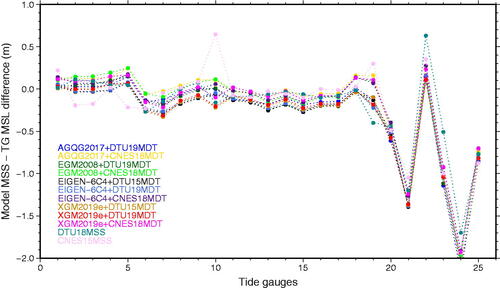
Figure 4 shows that ${\mathrm{h}}_{\mathrm{\text{MSL}}}$ obtained from the six AHO tide gauge (20–25) have very large differences with the modelled ${\mathrm{h}}_{\mathrm{\text{MSS}}}$ reaching nearly −2 m at Ila Point (24), although within ∼0.5 m at Troughton Island (20) and Long Island (22). The cause of this is not clear, but could include one, or a combination of, a blunder in the GNSS levelling connection (or booking/archiving error), a blunder in the tide gauge observations, or vertical datum (including the TGZ), or the short 30–60 day observation period. Alternatively, the error could be in the models, given the location of all six AHO tide gauges near Kalumburu (Figure 6) are along a complex coastline with a very large tidal range in bays with restricted flows from the ocean. In this context, the larger differences should be treated with caution, because the MSS and MDT model values may not have been well defined in these semi-enclosed bays and are within the ∼10 km ‘gap’ where radar altimetry is less reliable. This highlights the potential limitations in using models in some locations with more complex coastlines. Also of note in Figure 4 is the CNES15MSS spike at Cape Lambert (10) which is in the Dampier region (see Figures 2 and 6, Dampier inset map) which includes some complex coastline, and also the range of differences among MSS and N + MDT model ${\mathrm{h}}_{\mathrm{\text{MSS}}}$ at Derby (19). The tide gauge at Derby is located at the southern end of King Sound, which is a region of very large tides within a constricted ocean outlet, so it is a challenging area for the models.

Table 4 shows descriptive statistics that give further insight into the differences among the model ${\mathrm{h}}_{\mathrm{\text{MSS}}}$ and the tide gauge ${\mathrm{h}}_{\mathrm{\text{MSL}}}.$ The column with non-bold values show the statistics when all 25 tide gauges are included, while bold values show the results from the 19 tide gauges when the AHO tide gauges are removed from the computation. The ‘mean’ column indicates whether there is a systematic bias for each model ${\mathrm{h}}_{\mathrm{\text{MSS}}}.$ A zero mean indicates no systematic bias, whereas the non-zero mean suggest a systematic offset. When all 25 tide gauges are used, both the N+MDT and MSS model derived ${\mathrm{h}}_{\mathrm{\text{MSS}}}$ show biases of around 0.2 m – 0.3 m. This initially suggests that both altimetry-derived MSS and MDT may contain biases. However, when the AHO tide gauges are removed, the N+MDT model derived ${\mathrm{h}}_{\mathrm{\text{MSS}}}$ are all between −0.127 m and 0.046 m, with the MSS model ${\mathrm{h}}_{\mathrm{\text{MSS}}}$ magnitudes both within 0.06 m of zero.

Table 4. Descriptive statistics for differences between model ${\mathrm{h}}_{\mathrm{\text{MSS}}}$ from a range of N + MDT and MSS models and ${\mathrm{h}}_{\mathrm{\text{MSL}}}$ at tide gauges.

Model	Mean		Standard Deviation (SD)		RMS		Minimum		Maximum
AGQG17+DTU19MDT	–0.287	–0.062	0.536	0.096	0.608	0.114	–2.170	–0.184	0.149	0.149
AGQG17+CNES18MDT	–0.177	0.046	0.534	0.101	0.563	0.111	–2.056	–0.089	0.262	0.244
EGM2008+DTU19MDT	–0.299	–0.084	0.520	0.122	0.600	0.149	–2.089	–0.267	0.155	0.155
EGM2008+CNES18MDT	–0.189	0.024	0.518	0.122	0.551	0.125	–1.975	–0.172	0.250	0.250
EIGEN-6C4+DTU15MDT	–0.323	–0.127	0.492	0.103	0.588	0.163	–2.033	–0.280	0.151	0.076
EIGEN-6C4+DTU19MDT	–0.314	–0.117	0.492	0.103	0.584	0.156	–2.027	–0.264	0.158	0.079
EIGEN-6C4+CNES18MDT	–0.204	–0.009	0.490	0.104	0.531	0.105	–1.913	–0.168	0.278	0.174
XGM2019e+DTU15MDT	–0.321	–0.120	0.494	0.109	0.590	0.162	–2.046	–0.328	0.106	0.066
XGM2019e+DTU19MDT	–0.313	–0.110	0.495	0.108	0.585	0.154	–2.040	–0.312	0.113	0.069
XGM2019e+CNES18MDT	–0.202	–0.002	0.493	0.111	0.533	0.111	–1.926	–0.216	0.233	0.164
DTU18MSS	–0.204	–0.059	0.451	0.123	0.495	0.136	–1.701	–0.399	0.633	0.113
CNES15MSS	–0.199	0.005	0.531	0.201	0.567	0.201	–2.016	–0.231	0.647	0.647

The non-bold values are for all 25 tide gauges shown in Table 1 and used in Figure 4 while bold values are for the 19 tide gauges when all AHO tide gauges are removed (cf. Table 1). Units are metres.

The smallest RMS for the N+MDT derived MSS is 0.105 m for EIGEN-6C4(N)+CNES18MDT, with the combinations including the CNES18MDT generally having the smallest RMS. The standard deviation for all N+MDT derived MSS is generally ∼0.10 m, suggesting the difference in RMS is the result of the apparent ∼0.06 m bias between the DTU and CNES−CLS MSS models. This apparent negative bias of 0.05 m to 0.10 m in the DTU MDT models is not necessarily caused by the model itself, so should be viewed cautiously. Section ‘Comment on compatibility of the models and observations’ discussed some of the contributing factors to possible biases, including the tide gauge ${\mathrm{h}}_{\mathrm{\text{MSL}}}$ which may have different observation periods that are subject to sea level variability that may reach an upper bound of 0.15 m. Geoid errors in this coastal region may also contribute (for the N+MDT derived MSS), due to a combination of coastal gaps in terrestrial gravity observations, and errors in the altimetry gravity in the shallow water coastal region, which is discussed in Filmer et al. (2018).

Modelled LAT

The next set of results show a comparison between tide gauge ${\mathrm{h}}_{\mathrm{\text{LAT}}}$ (Equation 2(2) $${\mathrm{h}}_{\mathrm{\text{LAT}}}\approx {\mathrm{h}}_{\mathrm{\text{MSL}}}-{\Delta }_{\mathrm{\text{MSL}}‐\mathrm{\text{LAT}}}$$(2) ) which is considered representative of CD for this study, and ${\mathrm{h}}_{\mathrm{\text{LAT}}}$ estimated from the combined models (Equation 1(1) $${\mathrm{h}}_{\mathrm{\text{LAT}}}\approx {\mathrm{h}}_{\mathrm{\text{MSS}}}-{\Delta }_{\mathrm{\text{MSS}}‐\mathrm{\text{LAT}}}$$(1) ). The difference between tide gauge and models is notated as ${\Delta \mathrm{h}}_{\mathrm{\text{LAT}}}$ and is intended to gain insights into how accurately AUSHYDROID can be developed from models only. For this comparison, we selected a combination of geoid models EIGEN-6C4 and XGM2019e, and the two most recent MDT models DTU19MDT and CNES18MDT for the N+MDT derived ${\mathrm{h}}_{\mathrm{\text{MSS}}}$ with DTU18MSS and CNES15MSS used for the altimetry MSS derived ${\mathrm{h}}_{\mathrm{\text{MSS}}}.$ EIGEN-6C4 and XGM2019e are global gravity models, and have the advantage of including GOCE satellite gravity data, with Table 4 indicating small SD (and RMS with the CNES18MDT model), the apparently good results for the regional AGQG2017 notwithstanding. We use the ${\Delta }_{\mathrm{\text{MSS}}‐\mathrm{\text{LAT}}}$ height component from the FES2014b and TPXO9v5 OTMs for Equation (1)(1) $${\mathrm{h}}_{\mathrm{\text{LAT}}}\approx {\mathrm{h}}_{\mathrm{\text{MSS}}}-{\Delta }_{\mathrm{\text{MSS}}‐\mathrm{\text{LAT}}}$$(1) , plotting the ${\Delta \mathrm{h}}_{\mathrm{\text{LAT}}}$ comparisons at all 25 tide gauges in Figure 5, with descriptive statistics shown in Table 5. As per Section ‘Tide gauge and GNSS observations’ and ‘Models,’ we derive model and tide gauge ${\Delta }_{\mathrm{\text{MSS}}‐\mathrm{\text{LAT}}}$ from the four major constituents M₂, S₂, K₁, and O₁ over the same 5-year period where possible.

Figure 5. Comparison of ${\mathrm{h}}_{\mathrm{\text{LAT}}}$ derived from geoid(N)+MDT and MSS derived ${\mathrm{h}}_{\mathrm{\text{LAT}}}$ at 25 tide gauges.

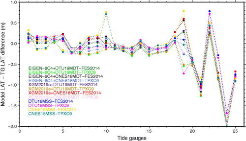
Table 5. Descriptive statistics for ${\Delta \mathrm{h}}_{\mathrm{\text{LAT}}}$ which is the difference between ${\mathrm{h}}_{\mathrm{\text{LAT}}}$ computed from models, and h_LAT computed from tide gauge records at the tide gauge location.

Models	Mean		Standard Deviation		RMS
EIGEN-6C4(N)+DTU19MDT–FES2014(LAT)	–0.234	–0.048	0.495	0.158	0.547	0.165
EIGEN-6C4(N)+DTU19MDT–TPXO9(LAT)	–0.307	–0.130	0.484	0.164	0.573	0.209
EIGEN-6C4(N)+CNES18MDT–FES2014(LAT)	–0.124	0.060	0.500	0.185	0.515	0.195
EIGEN-6C4(N)+CNES18MDT–TPXO9(LAT)	–0.197	–0.022	0.478	0.145	0.517	0.146
XGM2019e(N)+DTU19MDT–FES2014(LAT)	–0.233	–0.042	0.497	0.158	0.548	0.164
XGM2019e(N)+DTU19MDT–TPXO9(LAT)	–0.306	–0.123	0.484	0.160	0.573	0.202
XGM2019e(N)+CNES18MDT–FES2014(LAT)	–0.122	0.067	0.502	0.187	0.517	0.198
XGM2019e(N)+CNES18MDT–TPXO9(LAT)	–0.196	–0.015	0.478	0.142	0.517	0.142
DTU18MSS–FES2014(LAT)	–0.124	0.010	0.451	0.125	0.468	0.125
DTU18MSS–TPXO9(LAT)	–0.197	–0.072	0.457	0.188	0.498	0.201
CNES15MSS-FES2014(LAT)	–0.119	0.073	0.553	0.279	0.566	0.288
CNES15MSS-TPXO9(LAT)	–0.193	–0.008	0.512	0.197	0.547	0.198

The non-bold values are for all 25 tide gauges shown in Table 1 and used in Figure 4 while bold values are for the 19 tide gauges when all AHO tide gauges are removed (cf. Table 1). Units are metres.

Figure 5 shows both the N+MDT and the MSS derived ${\Delta \mathrm{h}}_{\mathrm{\text{LAT}}}$ to show similar behaviour to Figure 4 for the ${\Delta \mathrm{h}}_{\mathrm{\text{MSS}}}$ comparison. This suggests that both the FES2014b(LAT) and TPXO9v5(LAT) are a good representation of ${\Delta }_{\mathrm{\text{MSS}}‐\mathrm{\text{LAT}}}$ in this region. There is a noticeable positive and negative ‘spike’ at Derby tide gauge (19) which appears to exacerbate the large range at this tide gauge for the MSS comparison in Figure 4.

Table 5 shows the descriptive statistics for ${\Delta \mathrm{h}}_{\mathrm{\text{LAT}}}$ shown in Figure 5. If we remove the six AHO tide gauges near Kalumburu (cf. reasoning in section ‘Modelled MSS’), the 19 WADoT and PPA tide gauges present a clearer insight as to how ${\mathrm{h}}_{\mathrm{\text{LAT}}}$ can be modelled in a challenging coastal region such as north west Australia. All the models had mean difference <0.10 m, with the exception of two, which both included TPXO9v5(LAT) and DTU19MDT. All SD are below 0.20 m excluding CNES15MSS−FES2014b(LAT) (0.279 m). Most had RMS <0.2 m, with the lowest RMS the combination of DTU18MSS – FES2014b(LAT) with RMS of 0.125 m.

Figure 6 summarises the results in the test area by showing the spatial distribution of the EIGEN-6C4(N)+CNES18MDT ${\mathrm{h}}_{\mathrm{\text{MSS}}}$ and DTU18MSS–FES2014b(LAT) ${\Delta \mathrm{h}}_{\mathrm{\text{LAT}}}$ results at each tide gauge. Note the different vertical scale used for the inset locations and the full map. The ${\Delta \mathrm{h}}_{\mathrm{\text{LAT}}}$ in the bottom row for the PPA and AHO tide gauges are most instructive. The PPA Ashburton and WADoT Onlsow tide gauges ${\Delta \mathrm{h}}_{\mathrm{\text{LAT}}}$ are mostly between +0.05 m and +0.15 m, PPA Dampier and WADoT King Bay range from −0.24 m to +0.20 m, with ${\Delta \mathrm{h}}_{\mathrm{\text{LAT}}}$ at the 7 PPA tide gauges in the Port Hedland region between −0.14 m to + 0.04. Note the ${\Delta \mathrm{h}}_{\mathrm{\text{LAT}}}$ values in Figures 5 and 6 are ∼0.20 m higher at King Bay BN08 (8) and WADoT King Bay (9) which is not apparent in the ${\Delta \mathrm{h}}_{\mathrm{\text{MSS}}}$ in Figures 4 and 6 (insets), indicating that this is a difference in the OTMs. These results are in the Dampier region which Figure 6 (Dampier inset) suggests is a challenging area for the models.

Figure 6. Top left is the difference between ${\mathrm{h}}_{\mathrm{\text{MSS}}}$ computed at 25 tide gauges from EIGEN-6C4(N)+CNES18MDT and ${\mathrm{h}}_{\mathrm{\text{MSL}}}$ computed from the tide gauge record. Top right is the difference between ${\mathrm{h}}_{\mathrm{\text{LAT}}}$ computed from DTU18MSS and FES2014b(LAT) and ${\mathrm{h}}_{\mathrm{\text{LAT}}}$ computed from the tide gauge record. The middle row shows enlargements for the four clusters of tide gauges (shown in boxes (red in the online version) in the top row plots) for model ${\mathrm{h}}_{\mathrm{\text{MSS}}}$ minus tide gauge computed ${\mathrm{h}}_{\mathrm{\text{MSL}}}$ (as per top left), with the bottom row showing those same enlargements with model ${\mathrm{h}}_{\mathrm{\text{LAT}}}$ minus tide gauge computed ${\mathrm{h}}_{\mathrm{\text{LAT}}}$ (as per top right). The offshore dotted grey line in the inset boxes indicates the ∼10 km distance offshore adopted as the limit of reliable altimetry observations. Note the larger scale range for the enlargements on the right of rows 1 and 2 (Kalumburu) indicating the much larger differences for the northern-most AHO tide gauges.

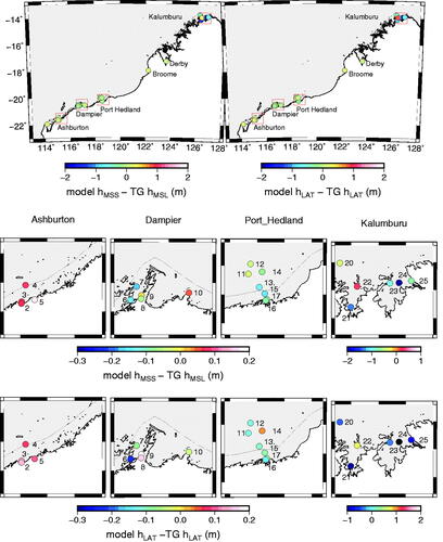
The AHO Kalumburu tide gauges ${\Delta \mathrm{h}}_{\mathrm{\text{LAT}}}$ are between −1.7 m and +0.8 m, which is up to an order of magnitude larger. Possible reasons for these larger differences for these tide gauges at these locations have been discussed earlier. The Figure 6 Port Hedland inset shows the tide gauges following the navigation channel out to sea across the 10 km line, so the changes in ${\Delta \mathrm{h}}_{\mathrm{\text{LAT}}}$ offshore offer an indication whether the modelled values degrade as they approach the coast. There is a change from around −0.15 m offshore to −0.05 m but no obvious change closer to the coast, which suggests that the modelled ${\Delta }_{\mathrm{\text{MSS}}‐\mathrm{\text{LAT}}}$ is reasonably reliable and there is no apparent gradient across the ∼10 km ‘gap’ in this area of open coast.

Discussion

This study provides background and context on the work towards an operational AUSHYDROID for Australia that would permit the multiple land and sea vertical datums around Australia to be connected. The fundamental quantity for this model is ${\mathrm{h}}_{\mathrm{\text{CD}}},$ which is the vertical separation between the reference ellipsoid and CD, represented in Australia by LAT over a specific epoch. To identify and evaluate the available models and observations to develop AUSHYDROID, we selected a study area in north west Australia. This is the first known evaluation of LAT estimated from MSS, geoid and MDT models in this challenging region.

Comparisons in the study area among a range of models and 19 tide gauge observations (after removing AHO tide gauges around Napier Broome Bay) indicated that modelled ${\mathrm{h}}_{\mathrm{\text{MSS}}}$ can replicate ${\mathrm{h}}_{\mathrm{\text{MSL}}}$ at the coastal tide gauges to 0.136 m RMS for DTU18MSS, and 0.201 m RMS for CNES15MSS. The RMS for the N + MDT approximation of MSS range from 0.105 m for EIGEN-6C4(N)+CNES18MDT, to 0.163 m for EIGEN-6C4(N)+DTU19MDT. We should be cautious in concluding which combination of models is the ‘best’ given that we are using only 19 tide gauges in a region with a very large tidal range, so that any apparent bias or larger RMS may be attributed to a range of factors. The MDT models have been computed by subtracting a different geoid model to the one we are using to restore the MSS. Both MDT are the result of specialised geoids, which have been tailored to fit with the MSS, and with a combination of filtering and ocean information assimilated to the MDTs to better define short scale ocean currents. Hence, the original MSS cannot be ‘exactly’ recovered, but these results indicate a close approximation is possible.

The addition of the OTMs to the comparisons to determine ${\mathrm{h}}_{\mathrm{\text{LAT}}},$ shown in Figure 5, indicate that FES2014b and TPXO9v5 provide similar agreement with the tide gauge ${\mathrm{h}}_{\mathrm{\text{LAT}}}$ in this study area (Table 5), although this depends on the combination of MDT, geoid or MSS model used with each. The differences for all tide gauges west of Derby, are much smaller, with Figures 5 and 6 indicating these are mostly between −0.20 m and + 0.20 m which suggest that in many Australian coastal regions, a combination of these models can be used to model ${\mathrm{h}}_{\mathrm{\text{CD}}}.$

There remains uncertainty around the suitability of the short term (30–60 day) AHO tide gauge installations for AUSHYDROID because these were only tested in a region that has very large tidal ranges and complex coastal characteristics. Short tide gauge records do not allow for as many tidal frequencies to be resolved from an analysis, and therefore lead to larger uncertainty in LAT and tide predictions in general. Tide gauges 20 (Troughton Island) and 23 (Carronade Island) both have differences <0.4 m, and are not within Napier Broome Bay, suggesting that the large differences may be attributable more to the MSS and OTM in this area than the short term tide gauges. It is possible that the models have not been well resolved in these semi-enclosed bays, which would contribute to the large differences, although those >0.5 m may relate to the tide gauge-GNSS connection.

Using more AHO short term tide gauges in the study across a wider range of coastal characteristics could have provided more insight, although uncertainty remains around the reliability of these tide gauge records based on the results in this study. Additionally, the lack of reliable (or any) GNSS levelling connections to these tide gauges has significantly reduced those that can be used in the study, and subsequently for AUSHYDROID. This remains a major impediment to developing a model to connect vertical land and sea datums, particularly in semi-enclosed bays where any solution requires tide gauges constraints.

Conclusions

This study to evaluate models and data for the development of AUSHYDROID has provided significant insights that will guide future work. A key conclusion is that ${\mathrm{h}}_{\mathrm{\text{MSS}}}$ derived from modelled MSS in combination with ${\Delta }_{\mathrm{\text{MSS}}‐\mathrm{\text{LAT}}}$ from an ocean tide model can estimate ${\mathrm{h}}_{\mathrm{\text{LAT}}}$ as per Equation (1)(1) $${\mathrm{h}}_{\mathrm{\text{LAT}}}\approx {\mathrm{h}}_{\mathrm{\text{MSS}}}-{\Delta }_{\mathrm{\text{MSS}}‐\mathrm{\text{LAT}}}$$(1) to <0.2 m along open coastline. The results suggest that MDT+N models can accurately realise MSS although may be problematic due to uncertainty as to how the geoid model was computed, in addition to the filtering and assimilated oceanographic information included in the MDT development.

In this study the combination of models could replicate ${\mathrm{h}}_{\mathrm{\text{MSS}}}$ at the tide gauges with an RMS of around 0.10 m, although this ranged up to ∼0.201 m. When we applied the ${\Delta }_{\mathrm{\text{MSS}}‐\mathrm{\text{LAT}}}$ from the OTMs to the ${\mathrm{h}}_{\mathrm{\text{MSS}}}$ as per Equation (1)(1) $${\mathrm{h}}_{\mathrm{\text{LAT}}}\approx {\mathrm{h}}_{\mathrm{\text{MSS}}}-{\Delta }_{\mathrm{\text{MSS}}‐\mathrm{\text{LAT}}}$$(1) , ${\mathrm{h}}_{\mathrm{\text{LAT}}}$ could be estimated with an RMS of between 0.125 m and 0.279 m, but mostly better than 0.20 m. However, the limitations of all models were evident in more complex coastal areas with challenging tidal signals such as Derby (19) within King Sound, Dampier South Reef (6) in the Dampier Archipelago and several AHO tide gauges in Napier Broome Bay where modelled ${\mathrm{h}}_{\mathrm{\text{LAT}}}$ was different to the tide gauge by as much as 2 m. The reasons for this may relate to models, observations and the GNSS levelling connection, and possibly a combination of all.

The small number of short-term tide gauges available is restricted due mostly to the GNSS levelling connections to the tide gauge being unavailable, or the archiving of the observations did not permit a reliable connection to enable the tide gauge observations to be transformed to a reference ellipsoid. This is crucial for the models to be connected to the modelled values in a proposed AUSHYDROID model. While the results of the study suggest that existing data can be used to develop AUSHYDROID in some coastal regions, there are limitations in the accuracy of the models and also the quality and number of observations that will need to be addressed to achieve an operational version of AUSHYDROID. These model and observation limitations are exacerbated in regions of complex coastline as experienced in part of our study area.

Acknowledgements

This research was performed under FrontierSI research project (FSI-4002) ‘A SCOPING STUDY AND ‘GAP’ ANALYSIS FOR THE DEVELOPMENT OF A NATIONAL HYDROID MODEL ("AUSHYDROID")’ funded by the Australian Hydrographic Office, Department of Defence.

The authors would like to both thank and acknowledge the contributions made by all FSI-4002 partners and participants involved in developing, reviewing and supporting the FrontierSI research project, including the Australian Hydrographic Office (AHO), Bureau of Meteorology (BOM), Geoscience Australia (GA), WA Department of Transport (WADOT), all of which made the research contained in this report possible. Figures 2–6 were plotted using the Generic Mapping Tools (Wessel et al. 2013).

We thank the AHO (Zarina Jayaswal, Chris Landon), WADOT (Tony Lamberto), PPA (Frans Schlack), and BOM (Andy Taylor, James Chittleborough) for providing tide gauge and GNSS data, Svetlana Erofeeva for providing the TPXO9v5 ocean tide model, and Ole Andersen for providing DTU MSS and MDT models.

FES2014 was produced by Noveltis, Legos and CLS and distributed by Aviso+, with support from CNES, and CNES-CLS. CNES-CLS MSS15 and MDT18 was obtained from Aviso+ as per Table 2.

The authors thank four anonymous reviewers and editor Dr Ron Li for their constructive comments which have helped us to improve the manuscript. We also thank Per Knudsen (DTU), Thomas Gruber (TUM) and Solène Jousset (CLS) for providing additional information on the development of the DTU and CNES-CLS MDT models.

Disclosure statement

No potential conflict of interest was reported by the author(s).

Data availability statement

Tide gauge data are available from the AHO, WADOT, PPA and BOM on request. AGQG2017 is available from Sten Claessens (Curtin University) on request. All other models are available as per the URL in Table 2, or by contacting the developers.

Additional information

Funding

This work was supported by The Australian Hydrographic Office, Department of Defence under Grant FSI-4002.

References

- Andersen, O. B., and P. Knudsen. 2009. “DNSC08 Mean Sea Surface and Mean Dynamic Topography Models.” Journal of Geophysical Research 114 (C11): C11001. https://doi.org/10.1029/2008JC005179
- Andersen, O. B., K. Nielsen, P. Knudsen, C. W. Hughes, R. Bingham, L. Fenoglio-Marc, M. Gravelle, M. Kern, and S. Padilla Polo. 2018a. “Improving the Coastal Mean Dynamic Topography by Geodetic Combination of Tide Gauge and Satellite Altimetry.” Marine Geodesy 41 (6): 517–545. https://doi.org/10.1080/01490419.2018.1530320
- Andersen, O. B., P. Knudsen, and L. Stenseng. 2018b. “A New DTU18 MSS Mean Sea Surface—Improvement from SAR Altimetry. 172.” In Proceedings of the 25 Years of Progress in Radar Altimetry Symposium, Ponta Delgada, São Miguel Island, Portugal, 24–29 September 2018. edited by J. Benveniste, and F. Bonnefond, vol. 172, 24–26. Portugal: Azores Archipelago.
- Andersen, O. B., S. K. Rose, P. Knudsen, and L. Stenseng. 2018c. “The DTU18 MSS Mean Sea Surface Improvement from SAR Altimetry.” In International Symposium of Gravity, Geoid and Height Systems (GGHS) 2, the Second Joint Meeting of the International Gravity Field Service and Commission 2 of the International Association of Geodesy, Copenhagen, Denmark, 17–21. September 2018.
- Bevis, M., W. Scherer, and M. Merrifield. 2002. “Technical Issues and Recommendations Related to the Installation of Continuous GPS Stations at Tide Gauges.” Marine Geodesy. 25 (1–2): 87–99. https://doi.org/10.1080/014904102753516750
- Bingham, R. J., K. Haines, and C. W. Hughes. 2008. “Calculating the Ocean’s Mean Dynamic Topography from a Mean Sea Surface and a Geoid.” Journal of Atmospheric and Oceanic Technology 25 (10): 1808–1822. https://doi.org/10.1175/2008JTECHO568.1
- Birol, F., N. Fuller, F. Lyard, M. Cancet, F. Niño, C. Delebecque, S. Fleury, et al. 2017. “Coastal Applications from Nadir Altimetry: Example of the X-TRACK Regional Products.” Advances in Space Research. 59 (4): 936–953. https://doi.org/10.1016/j.asr.2016.11.005
- Codiga, D. L,. 2011. Unified Tidal Analysis and Prediction Using the UTide Matlab Functions. Technical Report 2011-01. Graduate School of Oceanography, University of Rhode Island, Narragansett, RI. 59 pp. ftp://www.po.gso.uri.edu/ pub/downloads/codiga/pubs/2011Codiga-UTide-Report.pdf.
- Deng, X., Featherstone, W. E. Hwang, C., and Berry, P. A. M. 2002. “Estimation of Contamination of ERS-2 and POSEIDON Satellite Radar Altimetry Close to the Coasts of Australia.” Marine Geodesy. 25 (4): 249–271. https://doi.org/10.1080/01490410214990
- Egbert, G. D., and S. Y. Erofeeva. 2002. “Efficient Inverse Modelling of Barotropic Ocean Tides.” Journal of Atmospheric and Oceanic Technology 19 (2): 183–204. https://doi.org/10.1175/1520-0426(2002)019<0183:EIMOBO>2.0.CO;2
- Egbert, G. D., S. Y. Erofeeva, and R. D. Ray. 2010. “Assimilation of Altimetry Data for Nonlinear Shallow-Water Tides: Quarter-Diurnal Tides of the Northwest European Shelf.” Continental Shelf Research. 30 (6): 668–679. https://doi.org/10.1016/j.csr.2009.10.011
- Ekman, M. 1989. “Impacts of Geodynamic Phenomena on Systems for Height and Gravity.” Bulletin Géodésique 63 (3): 281–296. https://doi.org/10.1007/BF02520477
- Featherstone, W. E., J. F. Kirby, C. Hirt, M. S. Filmer, S. J. Claessens, N. J. Brown, G. Hu, and G. M. Johnston. 2011. “The AUSGeoid09 Model of the Australian Height Datum.” Journal of Geodesy 85 (3): 133–150. https://doi.org/10.1007/s00190-010-0422-2
- Featherstone, W. E., and M. S. Filmer. 2012. “The North-South Tilt in the Australian Height Datum is Explained by the Ocean’s Mean Dynamic Topography.” Journal of Geophysical Research 117 (C8): C08035. https://doi.org/10.1029/2012JC007974
- Featherstone, W. E., J. C. McCubbine, N. J. Brown, S. J. Claessens, M. S. Filmer, and J. F. Kirby. 2018. “The First Australian Gravimetric Quasigeoid Model with Location-Specific Uncertainty Estimates.” Journal of Geodesy 92 (2): 149–168. https://doi.org/10.1007/s00190-017-1053-7
- Fecher, T., R. Pail, and T. Gruber. 2017. “GOCO05c: A New Combined Gravity Field Model Based on Full Normal Equations and Regionally Varying Weighting.” Surveys in Geophysics 38 (3): 571–590. https://doi.org/10.1007/s10712-016-9406-y
- Filmer, M. S., and W. E. Featherstone. 2012. “A Re-Evaluation of the Offset in the Australian Height Datum between Mainland Australia and Tasmania.” Marine Geodesy.35 (1): 107–119. https://doi.org/10.1080/01490419.2011.634961
- Filmer, M. S., W. E. Featherstone, and M. Kuhn. 2010. “The Effect of EGM2008-Based Normal, Normal-Orthometric and Helmert Orthometric Height Systems on the Australian Levelling Network.” Journal of Geodesy 84 (8): 501–513. https://doi.org/10.1007/s00190-010-0388-0
- Filmer, M. S., C. W. Hughes, P. L. Woodworth, W. E. Featherstone, and R. J. Bingham. 2018. “Comparison between Geodetic and Oceanographic Approaches to Estimate Mean Dynamic Topography for Vertical Datum Unification: Evaluation at Australian Tide Gauges.” Journal of Geodesy 92 (12): 1413–1437. https://doi.org/10.1007/s00190-018-1131-5
- Förste, C., S. Bruinsma, R. Shako, J.-C. Marty, F. Flechtner, O. Abrikosov, C. Dahle, et al. 2011. “EIGEN-6 – A New Combined Global Gravity Field Model Including GOCE Data from the Collaboration of GFZ-Potsdam and GRGS-Toulouse.” Geophysical Research Abstracts 13, EGU2011-3242-2, EGU General Assembly.
- Foerste, C., S. L. Bruinsma, O. Abrykosov, J.-M. Lemoine, J. C. Marty, F. Flechtner, G. Balmino, F. Barthelmes, and R. Biancale. 2014. “EIGEN-6C4 the Latest Combined Global Gravity Field Model Including GOCE Data up to Degree and Order 2190 of GFZ Potsdam and GRGS Toulouse.” GFZ Data Services, 2015, 1. https://doi.org/10.5880/icgem.2015.1.
- Griffin, D. A., M. Herzfeld, M. Hemer, and D. Engwirda. 2021. “Australian Tidal Currents – Assessment of a Barotropic Model. (COMPAS v1.3.0 rev6631) with an Unstructured Grid.” Geoscientific Model Development 14 (9): 5561–5582. https://doi.org/10.5194/gmd-14-5561-2021
- ICSM. 2021. “Australian Tides Manual v6.0 Special Publication 9, PCTMSL.” https://www.icsm.gov.au/sites/default/files/SP9_Australian_Tides_Manual_V6.0.pdf.
- Iliffe, J. C., M. K. Ziebart, and J. F. Turner. 2007. “A New Methodology for Incorporating Tide Gauge Data in Sea Surface Topography Models.” Marine Geodesy 30 (4): 271–296. https://doi.org/10.1080/01490410701568384
- Iliffe, J. C., M. K. Ziebart, J. F. Turner, A. J. Talbot, and A. P. Lessnoff. 2013. “Accuracy of Vertical Datum Surfaces in Coastal and Offshore Zones.” Survey Review 45 (331): 254–262. https://doi.org/10.1179/1752270613Y.0000000040
- Jekeli, C. 2000. “Heights, The Geopotential and Vertical Datums.” Report No. 459. The Ohio State University, Columbus. http://www.geology.osu.edu/jekeli.1/OSUReports/reports/report_459.pdf.
- Keysers, J. H., N. D. Quadro, and P. A. Collier. 2013. “Vertical Datum Transformations across the Littoral Zone: Developing a Method to Establish a Common Vertical Datum before Integrating Land Height Data with Nearshore Seafloor Depth Data.” CRC-SI Report prepared for the Commonwealth Government of Australia, Department of Climate Change and Energy Efficiency. https://www.crcsi.com.au/assets/Uploads/Files/Vertical-Datum-Transformations-Across-the-Littoral-Zone-v1-3.pdf.
- Keysers, J. H., N. D. Quadros, and P. A. Collier. 2015. “Vertical Datum Transformations across the Australian Littoral Zone.” Journal of Coastal Research 31 (1): 119–128. https://doi.org/10.2112/JCOASTRES-D-12-00228.1
- King, M. 2014. “Priorities for Installation of Continuous Global Navigation Satellite System (GNSS) near to Tide Gauges.” Report to Global Sea Level Observing System (GLOSS). https://doi.org/10.13140/RG.2.1.1781.7049
- Knudsen, P., O. B. Andersen, and N. Maximenko. 2021. “A New Ocean Mean Dynamic Topography Model, Derived from a Combination of Gravity, Altimetry and Drifter Velocity Data.” Advances in Space Research 68 (2): 1090–1102. https://doi.org/10.1016/j.asr.2019.12.001
- Lyard, F. H., D. J. Allain, M. Cancet, L. Carrère, and N. Picot. 2021. “FES2014 Global Ocean Tide Atlas: Design and Performance.” Ocean Science 17 (3): 615–649. https://doi.org/10.5194/os-17-615-2021
- Mäkinen, J. 2021. “The Permanent Tide and the International Height Reference Frame IHRF.” Journal of Geodesy 95 (9): 106. https://doi.org/10.1007/s00190-021-01541-5
- Martin, R. J., and G. J. Broadbent. 2004. “Chart Datum for Hydrography.” The Hydrographic Journal 112: 9–14.
- Mayer-Gürr, T. and the GOCO Consortium, 2015. “The Combined Satellite Gravity Field Model GOCO05s.” Geophysical Research Abstracts Vol. 17, EGU2015-12364, 2015 EGU General Assembly 2015.
- Mills, J., and D. Dodd. 2014. “Ellipsoidally Referenced Surveying for Hydrography.” International Federation of Surveyors (FIG) publication 62.
- Moritz, H. 2000. “The Geodetic Reference System 1980.” Journal of Geodesy.74 (1): 128–133. https://doi.org/10.1007/s001900050278
- Mulet, S., M.-H. Rio, H. Etienne, C. Artana, M. Cancet, G. Dibarboure, H. Feng, et al. 2021. “The New CNES-CLS18 Global Mean Dynamic Topography.” Ocean Science 17 (3): 789–808. https://doi.org/10.5194/os-17-789-2021
- Nerem, R. S., F. J. Lerch, J. A. Marshall, E. C. Pavlis, B. H. Putney, B. D. Tapley, R. J. Eanes, et al. 1994. “Gravity Model Development for TOPEX/POSEIDON: Joint Gravity Models 1 and 2.” Journal of Geophysical Research 99 (C12): 24421–24447. https://doi.org/10.1029/94JC01376
- Parker, B., D. Milbert, and S. Gill. 2003. “National VDatum – The Implementation of a National Vertical Datum Transformation Database.” Proceedings of the U.S. Hydrographic Conference, Biloxi, Mississippi.
- Pavlis, N. K., S. A. Holmes, S. C. Kenyon, and J. F. Factor. 2012. “The Development and Evaluation of Earth Gravitational Model (EGM2008).” Journal of Geophysical Research 117 (B4): B04406. https://doi.org/10.1029/2011JB008916
- Petit, G., and B. Luzum (eds). 2010. “IERS Conventions 2010 (IERS Technical Note No. 36).” Frankfurt am Main, p 179.
- Pineau-Guillou, L., and L. Dorst. 2013. “Creation of Vertical Reference Surfaces at Sea Using Altimetry and GPS, Annales Hydrographiques.” Series 6 9 (777): 10.1–10.7.
- Ramm, D. R., C. J. White, A. H. C. Chan, and C. S. Watson. 2017. “A Review of Methodologies Applied in Australian Practice to Evaluate Long-Term Coastal Adaptation Options.” Climate Risk Management 17: 35–51. https://doi.org/10.1016/j.crm.2017.06.005
- Rio, M.-H., and F. Hernandez. 2004. “A Mean Dynamic Topography Computed over the World Ocean from Altimetry, in Situ Measurements, and a Geoid Model.” Journal of Geophysical Research 109 (C12): C12032. https://doi.org/10.1029/2003JC002226
- Robin, C., S. Nudds, P. MacAulay, A. Godin, B. De Lange Boom, and J. Bartlett. 2016. “Hydrographic Vertical Separation Surfaces (HyVSEPs) for the Tidal Waters of Canada.” Marine Geodesy 39 (2): 195–222. https://doi.org/10.1080/01490419.2016.1160011
- Roelse, A., H. W. Granger, and J. W. Graham. 1971. The adjustment of the Australian levelling survey 1970-1971. “Technical Report 12, Division of National Mapping.” Canberra, Australia.
- Schaeffer, P., I. Pujol, Y. Faugere, and A. Guillot. 2016a. “Picot. New Mean Sea Surface CNES CLS 2015 Focusing on the use of Geodetic Missions of Cryosat-2 and Jason-1, Oral Presentation OSTST 2016.” https://meetings.aviso.altimetry.fr/fileadmin/user_upload/tx_ausyclsseminar/files/GEO_03_Pres_OSTST2016_MSS_CNES_CLS2015_V1_16h55.pdf.
- Schaeffer, P., Y. Faugere, M.-I. Pujol, A. Guillot, and N. Picot. 2016b. The MSS CNES CLS 2015: Presentation and Assessment, Poster, Living Planet Symposium 2016. https://www.aviso.altimetry.fr/fileadmin/documents/data/products/auxiliary/MSS2015_poster_LivingPlanetSymposium2016.pdf.
- Schlack, F., and N. Hewitt. 2015. “Accurate Determination of Chart Depths by Establishing a Hydroid as a Port’s True Chart Datum.” Australasian Coasts & Ports Conference 2015: 22nd Australasian Coastal and Ocean Engineering Conference and the 15th Australasian Port and Harbour Conference, 2015, p.802–806.
- Seifi, F., and M. S. Filmer. 2023. “Residual M2 and S2 Ocean Tide Signals in Complex Coastal Zones Identified by X-Track Reprocessed Altimetry Data.” Continental Shelf Research 261: 105013. https://doi.org/10.1016/j.csr.2023.105013
- Slobbe, D. C., R. Klees, M. Verlaan, L. Dorst, and H. Gerritsen. 2013a. “Lowest Astronomical Tide in the North Sea Derived from a Vertically Referenced Shallow Water Model, and an Assessment of Its Suggested Sense of Safety.” Marine Geodesy 36 (1): 31–71. https://doi.org/10.1080/01490419.2012.743493
- Slobbe, D. C., M. Verlaan, R. Klees, and H. Gerritsen. 2013b. “Obtaining Instantaneous Water Levels Relative to a Geoid with a 2D Storm Surge Model.” Continental Shelf Research.52: 172–189. https://doi.org/10.1016/j.csr.2012.10.002
- Slobbe, D. C., R. Klees, and B. C. Gunter. 2014. “Realization of a Consistent Set of Vertical Reference Surfaces in Coastal Areas.” Journal of Geodesy 88 (6): 601–615. https://doi.org/10.1007/s00190-014-0709-9
- Slobbe, D. C., J. Sumihar, T. Frederikse, M. Verlaan, R. Klees, F. Zijl, H. H. Farahani, and R. Broekman. 2018. “A Kalman Filter Approach to Realize the Lowest Astronomical Tide Surface.” Marine Geodesy 41 (1): 44–67. https://doi.org/10.1080/01490419.22017.1391900
- Turner, J. F., J. C. Iliffe, M. K. Ziebart, and C. Jones. 2013. “Global Ocean Tide Models: Assessment and Use within a Surface Model of Lowest Astronomical Tide.” Marine Geodesy 36 (2): 123–137. https://doi.org/10.1080/01490419.2013.771717
- Vignudelli, S., F. Birol, J. Benveniste, L.-L. Fu, N. Picot, M. Raynal, and H. Roinard. 2019. “Satellite Altimetry Measurements of Sea Level in the Coastal Zone.” Surveys in Geophysics 40 (6): 1319–1349. https://doi.org/10.1007/s10712-019-09569-1
- Wessel, P., W. H. F. Smith, R. Scharroo, J. F. Luis, and F. Wobbe. 2013. “Generic Mapping Tools: Improved Version Released.” Eos, Transactions American Geophysical Union 94 (45): 409–410. https://doi.org/10.1002/2013EO450001
- Woodworth, P. L. 2012. “A Note on the Nodal Tide in Sea Level Records.” Journal of Coastal Research 280: 316–323. https://doi.org/10.2112/JCOASTRES-D-11A-00023.1
- Woodworth, P. L. 2022. “Providing a Levelling Datum to a Tide Gauge Sea Level Record.” Marine Geodesy 45 (1): 1–23. https://doi.org/10.1080/01490419.2021.1943577
- Woodworth, P. L., G. Wöppelmann, M. Marcos, M. Gravelle, and R. M. Bingley. 2017. “Why we Must Tie Satellite Positioning to Tide Gauge Data.” Eos, Transactions of the American Geophysical Union, 98. https://doi.org/10.1029/2017EO064037
- Woodworth, P. L., C. W. Hughes, R. J. Bingham, and T. Gruber. 2012. “Towards Worldwide Height System Unification Using Ocean Information.” Journal of Geodetic Science 2 (4): 302–318. https://doi.org/10.2478/v10156-012-0004-8
- Wöppelmann, G., S. Zerbini, and M. Marcos. 2006. “Tide Gauges and Geodesy: A Secular Synergy Illustrated by Three Present-Day Case Studies.” Comptes Rendus Geoscience 338 (14–15): 980–991. https://doi.org/10.1016/j.crte.2006.07.006
- Wunsch, C., and D. Stammer. 1997. “Atmospheric Loading and the Oceanic “Inverted Barometer” Effect.” Reviews of Geophysics 35 (1): 79–107. https://doi.org/10.1029/96RG03037
- Zingerle, P., R. Pail, T. Gruber, and X. Oikonomidou. 2020. “The Combined Global Gravity Feld Model XGM2019e.” Journal of Geodesy 94 (7): 66. https://doi.org/10.1007/s00190-020-01398-0