Summer snowline altitude gradients in Western Norway are influenced by maritime climate

ABSTRACT

Mountain snowline dynamics are relatively underreported with few studies exploring spatial snowline dynamics. Whilst clear regional-scale relationships between snowline location and temperature exist in European mountains, recent research at higher latitudes reports no response to climate change. In maritime mountains, snowlines occupy complex environmental gradients. Using timeseries of satellite data from Landsat missions 5–8 (151 images between 1984 and 2021), we explored sub-regional summer snowline dynamics across the maritime-continental climate gradient in the Western Norwegian mountains. We characterize spatio-temporal snowline altitude dynamics and investigate the climate factors altering snowline patterns. Summer snowline altitudes were found to increase inland at around double the rate of the 0°C summer isotherm. Data from the European Centre for Medium-Range Weather Forecasts (ECMWF) land component of the fifth generation of European Reanalysis (ERA5-Land), showed a potential ‘maritime-mountain’ effect with coastal orographic snowfall and cloud cover-induced surface solar downwelling radiation amplifying maritime-continental snowline altitude gradients alongside surface atmospheric temperature. This was replicated in the Canadian Rocky Mountains. Between 1984 and 2021, we found spatial summer snowline gradients in Norway decreased and propose multiple climate forcings are responsible, potentially masking links between snowlines and climate change. Although non-significant, the data also suggest regional summer snowline altitudes increased. This study demonstrates the complex spatial heterogeneity in snow-climate relationships and highlights how long-term snow dynamics can be queried using fine-grain (Landsat) resolution satellite data. We share our approach through a Google Earth Engine web-app that rapidly executes spatial snowline analyses for global mountain regions via a graphical user interface.

KEYWORDS:

• Snowline
• Norway
• climate change
• Landsat
• spatial analysis
• Google Earth Engine

Introduction

As the climate changes, alterations to snow dynamics threaten environments and society (Cherry et al. 2005; Edwards et al. 2007; Keenan and Riley 2018). With half the global population reliant on mountain freshwater (Rasul et al. 2020), one sixth originating from global snowmelt (Messerli et al. 2004; Barnett et al. 2005), it is particularly important to understand changes to snow. However, despite extensive research on the regional effects of climate change on snow dynamics and snowlines, little to no research explores the sub-regional scale spatial characteristics of snowlines and climate. The snowline is a non-glacial montane feature defined by Østrem (1974) as the boundary between snowpack and snow free areas. The summer snowline can be found during any of the meteorological summer months (June, July, and August in the Northern Hemisphere) and is the focus of this study. The snowline, therefore, sits at the balance point between snow ablation and accumulation (Barry et al. 1975); its altitude and location reflecting changes in climate through time (Beniston 2012). As a result, researching the spatial dynamics of snowline altitude and location at high resolutions may offer new insights into past and future local snowline change, its impacts on local water resources and ecology, and our ability to attribute snowlines and snow dynamics to climate forcings.

Of particular interest to spatial snowline research are coastal mountains as these partly encompass maritime-continental climate gradients which we argue produce a complex spatial forcing on snowlines. Verbyla et al. (2017) explore the impact of Alaskan regional snowline altitudes on Dall Sheep and, although ecologically focussed, they show regional snowline altitudes increase away from the Pacific Ocean. Glaciological literature also supports the concept of a maritime-continental relationship with Østrem (1973) commenting on higher glacial snowline altitudes near Calgary than Vancouver. Meier and Post (1962) show equilibrium contour altitudes increase inland in North America and, elsewhere, Heiskanen et al. (2002) and Racoviteanu et al. (2008) show links with temperature, sublimation, and snowfall. More direct evidence originates from older literature in Western Norway (Buch 1812; Forbes 1853; Vibe 1860; Richter 1896; Hansen 1902; Paschinger 1912). Although not accessible, results from these studies are reported by Ahlmann (1922) who quantified increases in snowline altitude inland. However, this assessment was based on few data points and methods possibly favouring well-defined, accessible snowlines. Early investigation from Buch (1812) linked the pattern to changing cloud cover, however, others, including Ahlmann (1922), Forbes (1853), and Paschinger (1912) supported temperature control as the principal driver, perhaps from the Massenerhebung effect. Crucially, Ahlmann (1922) found a 1°C increase in mean summer temperature (June-August at 500 m ASL) for every degree of longitude (∼50 km) was too small to entirely explain spatial snowline altitude trends in Western Norway and, therefore, also suggested a precipitation control was present.

Snow dynamics research in the European Alps shows declining snow extents since the early 1900s with projected decline under future emissions scenarios (Beniston 2012; Gobiet et al. 2014), especially at low-mid altitudes where temperature-enhanced ablation and rain-on-snow events occur (Serquet et al. 2011; Beniston 2012; Marty et al. 2017). Conversely, high altitude snow patterns remain unchanged, probably related to enhanced snowfall by higher, but still below −10°C, temperatures (Krasting et al. 2013). This is mirrored in Scandinavia by Hanssen-Bauer et al. (2015) and Räisänen (2021), who illustrate mixed control between temperature and precipitation (Dyrrdal and Vikhamar-Schuler 2009; Dyrrdal et al. 2013). Snowline research in the European Alps and Carpathian Mountains also reflects this with snowline altitudes increasing with isotherm altitudes (Krajčí et al. 2014; Hu et al. 2019b). This is expected as the summer or 0°C July isotherm is commonly used as an estimate of annual snowline altitude (highest altitude year-round) in both modern (de Quervain 1903; Troll 1961; Mengel et al. 1988) and palaeoclimate literature (Barry et al. 1975; Brakenridge 1978; Seltzer 1990). Specifically, Hu et al. (2020) found snowlines to retreat to higher altitudes in the European Alps between 1984 and 2018 at rates ranging from 4.17 to 8.76 ma⁻¹ and Hantel et al. (2012) report an altitude increase of 123–166 m°C⁻¹ between 1961 and 2011. However, recent research in northern European mountains shows high-latitude snowlines do not exhibit any temporal trends in altitude (Hu et al. 2019a). Therefore, high-latitude mountains may be affected by regional climatic drivers, potentially related to their maritime setting. A strong regional maritime-continental climate gradient across the Western Norwegian mountains may display such influences on snowlines which are hidden at larger regional-scales. With many global mountain ranges located in coastal settings, this is an important, yet understudied, aspect of the cryosphere which has important implications for resource management, local environmental dynamics, and successful climate modelling. This is echoed in a recent review by Hu et al. (2017, p. 29) who concluded Future studies should not only focus on […] cold region land surface dynamics in Europe, but also be directed towards a better understanding of these dynamics, especially as a response to ongoing climatic changes.

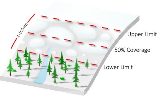
Current methods in snowline research are spatially coarse making them suitable for studying temporal climate and snowline change. For example, the Regional Snowline Elevation (RSLE) method (Krajčí et al. 2014; Hu et al. 2019b) relies on cumulative hypsography to produce a single regional snowline altitude. These rely on the more regular return periods associated with coarser-grain (MODIS) imagery as it aids clear sky observation and the creation of gap-filled snow cover products (e.g. MODIS and VIIRS (Hall et al. 2019)) (Parajka et al. 2010; Hu et al. 2019b). However, processing finer-grain (Landsat) imagery with new geo-computational techniques (e.g. Google Earth Engine (Gorelick et al. 2017)) is increasing the accessibility and inclusion of finer-grain data into long-term analyses (Hu 2020). For this study especially, this allows spatial snowline dynamics to be resolved easily through time. Crucially, finer-grain imagery offers reduced altitudinal uncertainty associated with smaller pixel footprints which are a necessity for comparing spatial snowline altitude change in steep mountainous terrain. As a result, spatial snowline studies with finer-grain (Landsat) imagery should increase our understanding on both spatial snowline dynamics but may also affect our understanding of temporal snowlines which are largely based on regional-scale methods and coarser-grain (MODIS) imagery. An important consequence of using finer-grain imagery, however, is that the greater detail uncovers the hypothetical nature of the snowline concept. This reveals the snowline to not always be a visibly abrupt line as is shown in coarser-grain (MODIS) imagery. The snowline instead sits within an ecotone-like gradient of diminishing patchy snow (Kleindienst et al. 2000) (Figure 1). UNESCO (1970) define the 50% coverage point within this ‘snow-tone’ as the snowline (Dozier and Painter 2004). Therefore, recovering the snowline from this snow-tone increases the methodological complexity when using finer-grain imagery.

Figure 1. The hypothetical nature of the snowline at finer spatial resolutions. Complex snow edges at the snow-tone stop easy definition and measurement of the snowline. A standardized snowline position is therefore necessary.

Thus, the sparse adoption of finer-grain (Landsat) spatial resolutions and the focus of literature on snowline dynamics through time means current methods are not suitable for exploring spatial snowline dynamics and their links to climate. As a result, few studies have characterized the spatial dynamics of snowlines empirically. This study attempts to do this by harnessing the cloud-computation platform of Google Earth Engine in order to deploy a novel spatially resolved regression-based approach to snowline delineation that preserves the spatial resolution of Landsat data. By pairing this with state-of-the-art ERA5-Land Climate Reanalysis, summer snowline and climate dynamics are resolved and compared for the last 37 years in the mountains of Western Norway. We aim to test the following hypotheses:

1. Summer snowline altitudes will increase linearly from the coast toward inland areas due to maritime-continental climate gradients in temperature, snowfall, and insolation.

2. Regional summer snowline altitudes will increase through time in line with increasing temperatures.

3. Summer snowline altitudes nearer the coast will increase through time at a reduced rate than further away from the coast due to maritime-mediated temperatures.

Study system

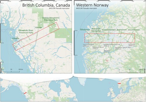
Recreating the transect used by Ahlmann (1922) to study snowlines, a 40 km wide by ∼225 km long transect was used stretching from the coast near Florø (61°42'N, 4°52'E) to inland near Otta (61°42'N, 9°07'E) (Figure 2). This positioning ensured continuous mountainous terrain and snowlines across the transect and at the coast. From a climatic perspective, the transect covered a zone where warm North Atlantic surface waters moderate coastal air temperatures, and the effects of continentality produce large seasonal temperature ranges inland (Ketzler et al. 2021). Orographic advection of this humid air produces high coastal precipitation of up to ∼3500 mm a⁻¹ and down to ∼300 mm a⁻¹ inland (Andreassen et al. 2012; Ketzler et al. 2021). Through the last 100 years, temperatures have increased by ∼0.8°C and since 1900, precipitation is now 20% higher (Hanssen-Bauer et al. 2015). The transect was therefore suitable to assess spatial maritime-continental climate gradients and temporal climate change. A secondary 40 km wide by ∼275 km long transect in British Columbia, Canada was located across the Rocky Mountains from near Kitkatla (53°45'N, 130°34'W) to near the Babine Mountains Provincial Park (54°53'N, 126°45'W) (Figure 2). This Canadian transect was chosen as, like the Norwegian transect, it included coastal mountains adjacent to warm sea surface temperatures (Amos et al. 2015) and the same Köppen-Geiger classifications (Cfb, Dfc, and ET) (Kottek et al. 2006), making it a suitable location to test the algorithm on maritime alpine systems elsewhere.

Figure 2. Map of Canadian and Norwegian transects (red). High altitude climate stations in italics in the Western Norway pane. Map data from Open Street Map, © OpenStreetMap contributors CC BY-SA 2.0.

Methods

Data processing

End-of-the-Ablation season

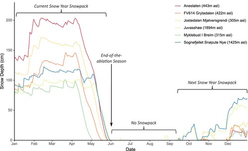
To determine the end-of-the-ablation season each year between 1982 and 2021, the first day of zero snow-depth was identified for each climate station with data from seNorge (NVE et al. 2022). The station with the latest occurrence determined the end-of-the-ablation season and was visually verified with snow-depth plots (see Figure 3). The mean of these dates was used to identify a suitable time of year to observe the summer snowline, around which a fixed image collection window was selected. A 16-day image collection window was used to allow satisfactory data density, cloud avoidance, and transect coverage whilst reducing temporal uncertainty as much as possible. For testing in Canada, an arbitrary summer date of 2021/07/01 near the end of the Canadian ablation season is used based on glaciological studies (Tennant and Menounos 2013; Marshall and Miller 2020).

Figure 3. Method to determine the end-of-the-ablation season illustrated using example seNorge observed snow depths from high altitude climate stations in the Norwegian transect.

Snow edge algorithm

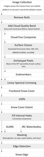
Measuring detailed changes in snowline dynamics through time requires an efficient procedure that can be applied to hundreds of satellite scenes whilst still preserving spatial resolution. Landsat missions 4–8 provide a unique dataset spanning 1982–2021 at 30 m spatial resolution (Wulder et al. 2019). Tier 1 atmospherically corrected surface reflectance scenes from WRS paths 199–201 and row 17 were used in the Norwegian transect. To resolve the snowline, a per-pixel fractional snow cover algorithm using linear spectral unmixing was developed. Linear spectral unmixing is widely used in snow cover products (SnowStar (Andersen 1982; Solberg and Andersen 1994), MODIS fractional snow cover (Hall et al. 1995), and MODIS snow covered area and grain size (Painter et al. 2009)) and offers notable benefits for quantifying snow extent, being described by Painter et al. (1998, p. 331) as superior to using band ratios. The approach estimates the fractional snow cover within the footprint of the pixel unlike band ratioing methods which suffer from the mixed pixels problem (Rosenthal and Dozier 1996; Painter et al. 1998). Linear spectral unmixing is applicable to non-forested snowpacks where summer snowlines in Norway persist and is easily operationalized on the cloud-computing platform of Google Earth Engine (Gorelick et al. 2017) which also offers integrated access to satellite and environmental datasets.

The algorithm is illustrated fully in Figure 4 with an example scene in Figure S1. In essence, linear spectral unmixing is applied to each scene using endmembers obtained from archetypal band values from multiple band ratio-derived surface cover classes. These surface cover classes are: snow from the Snow Water Index (SWI) (Dixit et al. 2019), vegetation from the Green Vegetation Index (GVI) (Kauth and Thomas 1976), water from the reciprocal of a combined Modified Normalized Difference Water Index (MNDWI) (Xu 2006) and Normalized Difference Water Index (NDWI) (Gao 1996), and rock from the Normalized Difference Built-up Index (NDBI) (Zha et al. 2003). This produces fractional snow cover from which values ≥50% determine snow extent (UNESCO 1970), the perimeter of which is the snow-edge. Snow-edges are masked to remove frozen lakes (EU JRC Waterbodies (Pekel et al. 2016)), ice caps and glaciers (GLIMS (Raup et al. 2007)), and clouds. The cloud mask is based on a sum average Gray-Level Covariance Matrix (GLCM) texture analysis (Haralick et al. 1973) and is buffered to capture thin cloud to avoid interference with snow cover percentage estimates during unmixing. This circumvents most pixel-level misclassifications between cloud and snow and avoids using the Landsat CFmask, which was too aggressive, repeatedly misclassifying the snow-tone, where the snowline resides, as cloud. At each snow-edge, altitude, aspect, and slope were calculated from the Advanced Land Observing Satellite (ALOS) World 3D–30 m (AW3D30) terrain model (EORC and JAXA 2017). Snowline altitude uncertainties (u) were calculated by combining the AW3D30 elevation error of ±5 m in Scandinavia (E_e) (Karlson et al. 2021) with the trigonometric function between slope angle (θ) and the Landsat horizontal translation error of ±12 m (E_t) (Rengarajan et al. 2020) (see Equation (1)). (1) $\mathrm{u}=\tan (\theta )\ast {\mathrm{E}}_{\mathrm{t}}+{\mathrm{E}}_{\mathrm{e}}$(1)

Figure 4. Stepwise procedure used by the snow-edge algorithm.

Climate processing

Via Google Earth Engine, the ERA5-Land Climate Reanalysis was used to provide hourly climate data at 11,132 m latitudinal resolution (Muñoz-Sabater et al. 2021). Since 1981 to present, these cover the time range of Landsat missions 4–8 and show agreement with observed weather and climate (Babar et al. 2019; Pelosi et al. 2020; Keller and Wahl 2021; Velikou et al. 2022, p. 1). Scandinavian mountain precipitation and temperature patterns are reproduced faithfully (Bandhauer et al. 2022; Velikou et al. 2022). At the centre of each grid square of the ERA5-Land Climate Reanalysis, 2 m atmospheric temperature, surface snowfall, and surface solar downwelling radiation were collected within the Norwegian transect. Temperature data were corrected to sea-level altitude using the mean AW3D30 elevation for each climate grid square and an approximate lapse rate of 0.65°C per 100 m altitude (Ketzler et al. 2021). The mean was calculated for the meteorological seasons within each ‘snow year’. A snow year starts in autumn as the first snowfall occurs then, melting during the ablation season in the spring and summer of the following year. Owing to the TCo1279 gaussian grid used by the ECMWF (Malardel et al. 2015), the longitudinal resolution is ∼5 km at the latitude of the Norwegian transect.

Data analysis

Spatial snowlines and climate

Predictions of spatial summer snowline altitude were produced from ordinary least squares (OLS) regressions of snow-edge altitudes against distances from the coast. Prediction uncertainty was calculated using the 95th and 5th percentiles of mean snow-edge altitudes across 2° aspect bins. This process was applied to each year of snow-edge data from the Norwegian transect, with the results compared to historical snowline altitude data from Ahlmann (1922, p. 11) across the same area. The same process was applied to the Canadian transect to assess algorithm performance and spatial snowline patterns for another coastal mountain range. For each year between 1981 and 2021, a maritime-continental climate gradient for snowfall, sea-level-corrected temperature, and surface solar downwelling radiation against distance from the coast across the Norwegian transect was characterized using OLS or nth order polynomial regressions. Regression type was dependent on data patterns, residuals, and anova variance tests. A temporal mean regression gradient of sea-level-temperature against distance from coast was calculated for 1981–2021 and converted to an altitude by distance gradient using the approximate environmental lapse rate of 0.65°C per 100 m (Ketzler et al. 2021). This calculated the 0°C summer isotherm for comparison to the predicted snowline altitude gradient.

Temporal snowline and climate

Each year, regional summer snowline altitude estimates were calculated using the predicted snowline gradients and a fixed transect distance. This fixed distance was found from the mean of each year’s median snow edge distance. Altitude errors used the aspect-derived uncertainty calculated for spatial snowline predictions. For each year, mean snowfall, sea-level-temperature, and surface solar downwelling radiation were calculated from the spatial climate data. OLS regressions and Mann-Kendall trend tests were performed on both regional snowline altitude and mean climate variables against the median time of image acquisition and season, respectively. Mann-Kendall tests were performed in 10,000 Monte Carlo simulations in order to provide a robust assessment of snowline and climate patterns through time given the limited number of data points and in case of interannual patterns (R package: Astrochron v1.1, R version: 4.1.1, Meyers (2014)). A mean regional snowline altitude estimate was calculated for the centre of Jostedalsbreen (∼100 km inland along the Norwegian transect) for comparison to Hu et al. (2019a).

Temporal snowline gradients

As in Temporal Snowline and Climate, an OLS regression and 10,000 Monte Carlo simulations of Mann-Kendall trend tests were used to assess the change in predicted snowline gradients against median imagery dates between 1982 and 2021 across the Norwegian transect. Errors in the predicted snowline gradients were derived from the 95th percentile of 10,000 bootstrap resamples of snow-edge data, performing snowline altitude predictions (R package: Boot v1.3-28, R version: 4.1.1, Ripley (2021) and Davison and Hinkley (1997)).

Algorithm validation

As the snowline is a hypothetical concept defined by the 50% coverage point across a snow-tone, validating altitude predictions is challenging. Instead, cross-validation of snow extents between the study algorithm and MOD10A1 product were used to assess accuracy. MOD10A1 is used as most snowline delineation methods from the current literature use MODIS and, as the 2nd most widely used (18%) platform in snow dynamics research (Hu et al. 2017), it has also been repeatedly validated with ∼92–93% accuracy under clear sky conditions (Hall et al. 2019; Riggs and Hall 2020). Its rapid revisit period of ∼2 days and large swath (2300 km) make it suitable for cross-validating Landsat imagery that has a smaller footprint and a less frequent revisit period. A new Landsat 4–8 image collection over the Norwegian transect (WRS path: 199–201, row: 17) with below 10% cloud cover was curated irrespective of date. Cloud-filtering is used as MOD10A1 is a gap-filled product (Hall et al. 2019) whilst the study algorithm is not. Each Landsat image was paired with a MOD10A1 snow extent raster for the same day. A truncated version of the study algorithm was used to find snow extent and sun elevation for each Landsat image. Percentage snow extent for each image pair was retrieved within the Landsat image footprint and mean absolute error (MAE) was calculated. OLS regression of the study algorithm against MOD10A1 snow extents was performed.

Results

Data summary

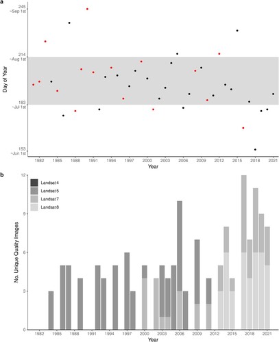
For Norway, most end-of-the-ablation season dates were in July (Figure 5a) with a mean of the 196th day of the year (~15th July). A 16-day imagery collection window was centred around this, starting from 8th July. For these dates, 151 Landsat images were found for the Norwegian transect with a mean of 5.8 images per year (excluding missing years). No data were recovered from Landsat 4 and select years (Figure 5b). Validation imagery totalled 122 images.

Figure 5. (a) End-of-ablation season dates from 1981 to 2021 for the Norwegian transect. Grey box represents July. Red points are used for years with no recovered Landsat data during 8–23 July. (b) Landsat image densities for each year’s 16-day window after 8th July.

Norwegian snowline altitude gradient

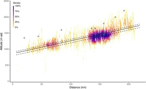
Snowline altitudes showed a significant and positive linear relationship with distance away from the coast continuously between 1984 and 2021 (Figure 6). The mean snowline altitude gradient across all study years increased away from the Western Norwegian coast at 4.49 m km⁻¹ ±0.44 (1σ). The mean snowline gradient predicts a minimum snowline altitude of 792 m at 0 km (coast) and a maximum altitude of 1802 m at 225 km (inland). 99% of snow-edge data points had an altitudinal error of ±≤12.2 m. Data from Ahlmann (1922) showed a close similarity with datapoints near the upper snow-tone resolved by this study (Figure 6).

Figure 6. Example plot from 2017 (Landsat 7/8) depicting snow-edge altitude against distance from the Western Norwegian coast (coloured points). Densities derived from neighbourhood kernel. Snowline altitude prediction from OLS regression (solid line) (adj.r2_(601031) = 0.58, p<.005) with uncertainty (dashed) calculated from 95th and 5th percentiles of mean snow-edge altitudes across 2° aspect bins. Data are accompanied by snowline altitude observations reported by Ahlmann (1922) (cross).

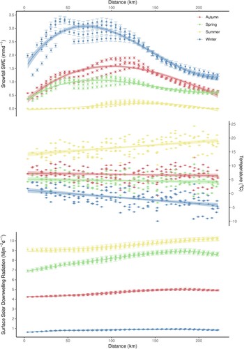
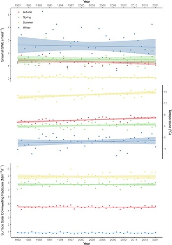
Temperature, snowfall, and surface solar downwelling radiation showed a maritime-continental climate pattern was present between 1981 and 2021 (Figure 7). Notably, winter snowfall near the coast (20–100 km) was highest with a mean maximum of 4.2 mm of snow water equivalent (SWE) per day ±1.7 (1σ) averaged from all years, whereas inland (225 km) it was lowest at a mean minimum of 0.9 mm SWE per day ±0.3 (1σ) averaged from all years. Across all years, summer and spring surface solar downwelling radiation increased away from the coast, especially in the latter. Yearly regressions of the seasonal sea-level-temperatures showed the mean range across all years to be greater inland (21.83°C at 225 km) than at the coast (12.44°C at 0 km). Only summer temperatures increased away from the coast at 0.015°C km⁻¹ (1°C per 66.79 km). The equivalent isothermal altitude gradient was 2.30 m km⁻¹.

Figure 7. Mean daily sea-level-temperature, snowfall, and surface solar downwelling radiation for each meteorological season in the 2018 snow year against distance. Error bars indicate SEM. Confidence intervals at 95%. Due to the latitudinal resolution of the ERA5-land Climate Reanalysis, climate data were extracted from multiple latitudinal grid rows within the transect. This produced multiple separate spatial curves for each season of each climate variable as is particularly visible for snowfall.

Norwegian regional snowline altitudes through time

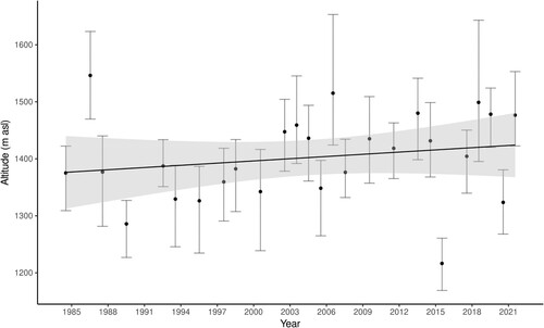
Regional summer snowline altitudes showed an increasing, but non-significant, temporal trend (adj.r²₍₂₄₎ = −0.003, p = .347; Kendall’s τ₍₉₉₉₈₎ = 0.194, p = .158). The OLS regression shows the regional snowline altitude increased by 13 m per decade (48 m between 1984 and 2021) with a mean altitude of 1402.32 m ±76.17 (∼5%) (1σ) (Figure 8). A mean regional snowline altitude for central Jostedalsbreen was estimated at 1241.26 m ±79.71 (1σ).

Figure 8. Regional snowline altitudes for the Norwegian transect between 1984 and 2021. OLS regression (adj.r2₍₂₄₎ = −0.003, p = .347; Kendall’s τ₍₉₉₉₈₎ = 0.194, p = .158) (black) is accompanied by 95% confidence intervals (grey). Error bars constructed from the aspect uncertainty of each yearly snowline altitude prediction.

Snowfall, sea-level-corrected temperature, and surface solar downwelling radiation reported no significant change through time aside from mean autumn and summer temperatures (Figure 9). OLS regression and Kendall’s Tau reported significant temperature relationships of 0.396°C per decade in autumn (adj.r²₍₃₈₎ = 0.31, p<.005; Kendall’s τ₍₉₉₉₈₎ = 0.40, p<.005) and of 0.462°C per decade in summer (adj.r²₍₃₈₎ = 0.23, p<.005; Kendall’s τ₍₉₉₉₈₎ = 0.32, p<.005). Winter snowfall exhibited no patterns and large variance at ±1.03 mm SWE (1σ) (±40%) about the mean of 2.56 mm SWE per day averaged from all years.

Figure 9. Mean daily sea-level-temperature, snowfall, snowmelt, and surface solar downwelling radiation values for meteorological seasons between 1981 and 2021. Confidence intervals at 95%.

Norwegian snowline altitude gradients through time

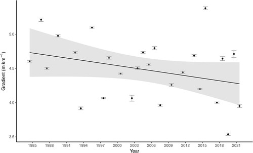
Summer snowline altitude gradients between 1984 and 2021 showed a decreasing temporal trend of 0.25 m km⁻¹ per decade which reported as significant under the Mann-Kendall trend test (OLS adj.r²₍₂₄₎ = 0.064, p = .114; Kendall’s τ ₍₉₉₉₈₎ = −0.194, p = .044) (Figure 10). Gradient variability ranged from 3.54–5.38 m km⁻¹, however, data were clustered about the mean gradient of 4.49 m km⁻¹ ±0.44 (∼10%) (1σ).

Figure 10. Snowline altitude gradients for the Norwegian transect between 1984 and 2021. Error bars produced from the 95% confidence interval of regressions from 10,000 bootstrap samples. OLS regression (adj.r2₍₂₄₎ = 0.064, p = .114; Kendall’s τ₍₉₉₉₈₎ = −0.194, p = .044) is accompanied by 95% confidence intervals.

Canadian snowline gradient

To assess the generalisability of the algorithm to maritime alpine systems elsewhere, testing was conducted in British Columbia, Canada. The algorithm successfully delineated snow-edges and predicted the snowline for Landsat 8 imagery over the Canadian transect between 2021/07/01-16 (Figure S2). OLS regression showed significant snowline altitude increase away from the Pacific Ocean at 4.55 m km-1 (adj.r²_(696980) = 0.49, p<.005). A large altitudinal range in snow-edge data was present between 50 and 150 km. An annotated depiction of this is displayed in Figure S3.

Validation

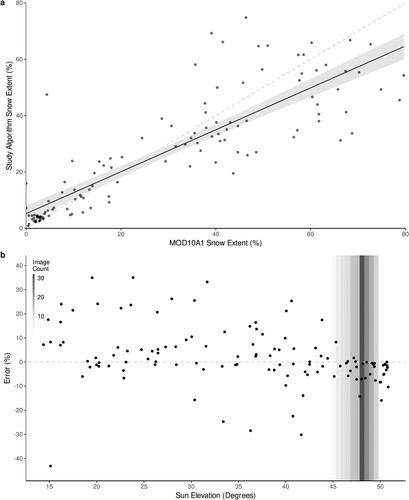
Study algorithm performance was similar to MOD10A1 with increasing spread at greater snow extents (Figure 11a). Per-image errors against sun elevations showed increasing spread toward lower elevations (Figure 11b). For all sun elevations, the MAE was 8.31% and for the sun elevations of the Norwegian transect imagery (44.3–50.0°) the MAE was 3.85% (Figure 11b).

Figure 11. (a) The study algorithm derived snow extent percentage against MOD10A1. OLS regression (solid) (adj.r2₍₁₂₀₎ = 0.74, p<.005) and 95% confidence intervals (grey). Dashed line indicates 1:1 line. (b) Errors of percentage snow extent for the study algorithm against the MOD10A1 algorithm for each validation image by sun elevation. Dashed line indicates 0% difference. Bars indicate the number of Norwegian transect images present by sun elevation.

Discussion

Snowline altitude gradient

The predicted summer snowline altitude increased away from the Western Norwegian coast in every year that yielded data with a mean gradient of 4.49 m km⁻¹ (Figure 10). This is visually similar to historical data from Ahlmann (1922) in the same area which, when superimposed, track the upper limit of the snow-tone resolved by this study (Figure 10). Near the 2021 end-of-the-ablation season in British Columbia, Canada, the predicted snowline shows a similar gradient to the Norwegian mean at 4.55 m km⁻¹, suggesting the phenomenon is present elsewhere.

The climatic explanation of these gradients relies on the environmental lapse rate and pioneering work of Ahlmann (1922) who developed the idea that the July summer 0°C isotherm indicates the altitude where the thermal energy imparted from the atmosphere to the snowpack is equal to the energy required to ablate the yearly total snowfall. This as an approximation of snowline altitude both in modern (de Quervain 1903; Troll 1961; Mengel et al. 1988) and palaeoclimate literature (Barry et al. 1975; Brakenridge 1978; Seltzer 1990). Therefore, the mean summer temperature gradient in Norway (0.015°C km⁻¹) should be similar to the mean summer snowline gradient found by this study. Converting the temperature gradient to the 0°C summer isotherm reports an altitudinal gradient of 2.30 m km⁻¹. This is around half (∼51%) that of the predicted mean snowline gradient (4.49 m km⁻¹). Work by Hantel et al. (2012) on climate change in the European Alps estimates snowline altitude to have increased through time by 123 m°C⁻¹. Mapping this to the spatial temperature change across the Norwegian transect would predict an isotherm and snowline altitude gradient of 1.80 m km⁻¹. Temperature measurements by Ahlmann (1922) place a historical summer temperature gradient at 1°C per 50 km (0.02°C km⁻¹) or 3.07 m km⁻¹. These temperature gradients are lower than the predicted snowline gradient found by this study and, as a result, we suggest summer temperatures in Western Norway do not operate alone to provide the climate driver necessary to produce the snowline altitude gradient. Therefore, we support Ahlmann (1922) in suggesting that other factors aside from temperature must be present in order to enhance the snowline gradient in Western Norway.

We suggest this enhancement could be produced by snowfall and surface solar downwelling radiation. Patterns in the ERA5-Land Climate Reanalysis show snowfall decreases away from the coast, especially in winter, whereas surface solar downwelling radiation increases away from the coast in spring and summer. These patterns agree with other research (Skartveit and Olseth 1986; Hanssen-Bauer 2005; Hanssen-Bauer et al. 2015; Ketzler et al. 2021). They occur from the orographic advection of warm, humid air over the coastal Scandinavian Mountains originating from the warm thermohaline circulation and North Atlantic extratropical cyclones (Sandvik et al. 2018). Therefore, proximity to the ocean (lake/sea-effect snowfall) (Doesken and Judson 2000) and the Foehn effect create an eastward precipitation shadow inland (Andreassen et al. 2012; Ketzler et al. 2021). This enhances the snowline altitude gradient by increasing the energy required to ablate the thicker snowpack at the coast, depressing coastal snowline altitudes. Conversely, there is a reduction in the energy required to ablate the snowpack in inland areas, increasing inland snowline altitudes. The effect of orographic advection also increases coastal cloud cover – a common phenomenon in Western Norway (Skartveit and Olseth 1986; Ketzler et al. 2021). This decreases surface solar downwelling radiation, snowpack energy input, and therefore coastal snowmelt as Buch (1812) suggested. In agreement with Stjern et al. (2009), the study data show reduced coastal surface solar downwelling radiation occurs mostly in spring and summer. Research suggests this is caused by seasonal storm frequencies, cyclonic/anticyclonic weather patterns, and diminished atmospheric sunlight penetration during low winter sun elevations (Parding et al. 2016; Ketzler et al. 2021). Comparison to one year of snowline data in Canada shows a similar predicted snowline gradient and so it supports this hypothesis. This is consistent with Scandinavian snow dynamics literature which demonstrates heterogenous snowpack control from temperature and snowfall (Dyrrdal et al. 2013; Hanssen-Bauer et al. 2015; Räisänen 2021).

Regional snowline altitudes through time

Contrary to Hu et al. (2019a), regional snowline altitudes showed an increasing trend through time, although it is weak and non-significant. The mean altitude estimate for Jostedalsbreen (∼100 km inland) was 1241 m ±80 m (1σ) which is very similar to the July estimate of ∼1247 m ±145 m (1σ) digitized from Hu et al. (2019a) between 1982 and 2017. The data from this study, however, are constrained to a smaller altitudinal range. Our Jostedalsbreen estimates may therefore have benefited from calculating snowline gradients using data from the entire Norwegian transect.

If the regional snowline has risen in altitude, then we suggest increasing summer and autumn temperatures, both at the coast and inland, are responsible as is shown in our data and by other literature in the European Alps (Hantel et al. 2012; Hu et al. 2020). However, the observed 13 m increase in regional snowline altitude per decade is smaller than expected. Assuming a spatially constant environmental lapse rate of 0.65°C per 100 m (Ketzler et al. 2021) we would expect the regional snowline altitude to increase between ∼60–70 m per decade under a 0.396–0.462°C per decade increase in autumn and summer temperatures, respectively. This would be similar to the increase in altitude found by studies in the European Alps (Hu et al. 2020). Therefore, even though it is not shown by the climate data, we also suggest other factors are present to temper the effects of increasing temperature and cause this disconnect. As, for the last two decades, snowfall has been shown to increase in Western Norway above 1350 m and decrease below (Hanssen-Bauer et al. 2015), it may be that the proportion of the snowline that exists above is increasing in altitude at a slower rate than the proportion below, or not at all. Therefore, when the snowline gradient data are used to find regional snowline altitude values, the effect of increasing temperature may be diluted, hiding sub-regional snowline trends. This demonstrates the importance of monitoring snowlines and climate at sub-regional scales. Large amounts of noise and observational uncertainties in these data also restrict our conclusions.

Visually the data may show a snippet of a sinusoidal pattern, perhaps in relation to phenomena like the North Atlantic Oscillation and Atlantic Multidecadal Oscillation, however, the observational uncertainties and short time period make it difficult to draw any further conclusions.

Snowline altitude gradients through time

The snowline altitude gradients show a decreasing temporal trend of 0.25 m km⁻¹ per decade (significant under the Mann-Kendall Trend test), moving the snowline closer to that of the summer isotherm gradient. Such a pattern suggests that the inland snowline is either being depressed or is rising more slowly than the coastal snowline. For this to occur the spatial climate patterns across the Norwegian transect must change through time.

Climate change in Norway is increasing inland temperatures at a greater rate than in coastal areas (Hanssen-Bauer et al. 2009, 2015; Ketzler et al. 2021). These temperature changes alone would, therefore, have the opposite effect on the snowline, increasing the gradient instead. Ground snowpack observations by Skaugen et al. (2012) show decreasing SWE trends at low altitudes and positive trends at high altitudes. Dyrrdal et al. (2013) show snow depths are decreasing in ‘warm-winter’ areas (coastal) and increasing in ‘cold-winter’ areas (inland and high-altitude plateaus). This is reflected by Hanssen-Bauer et al. (2015) who find snowfall has been decreasing below altitudes of 1350 m for the past two decades and the number of snow cover days is projected to decrease in the future with the greatest reduction in coastal areas of Western Norway. Therefore, over 1350 m in the inland mountains around Breheimen and Jotunheimen, snowfall may be acting against increases in temperature by maintaining or even depressing the snowline, whereas at lower elevations near the coast, decreases in snowfall below 1350 m paired with increasing temperatures may be moving the snowline to higher altitudes. We suggest that together these drivers may be decreasing the snowline gradient.

Other factors such as increased cyclonic conditions, cloud cover and opacity (Hanssen-Bauer et al. 2003; Parding et al. 2014; Devasthale et al. 2022), and precipitation and rain-on-snow events (Hanssen-Bauer et al. 2015) may affect the snowline gradient too. Skaugen et al. (2012) also note how variations in SWE trends are especially influenced by the North Atlantic Oscillation as supported by glacier mass balance studies (Nesje et al. 2000; Marzeion and Nesje 2012). This adds supplementary support for the spatially informed conclusion that, alongside temperature, multiple climate factors such as snowfall are responsible for determining snowline altitudes in Western Norway.

These observations also demonstrate that the amplitude and strength of in situ observations of snow depth trends do not necessarily reflect that of snowlines and snow cover area. Trends in snowlines and snow cover area may not be easily distinguishable from interannual snow depth variability and other climate factors that exert control. This is compounded by snow depth observations being able to show snow trends at higher resolutions as well. Therefore, snowline altitude and snow cover area are limited in this scope. However, satellite derived snowline altitude and snow cover area measurements may offer a readily accessible insight into the effects of multiple climate variables that measuring variations in only snow depths cannot. This may be especially useful where in situ monitoring is sparse. Perhaps, snowline altitude observations can even be used to aid the evaluation of high-resolution climate models as the effects of a changing climate on the snowline should also be replicated to match that of the observed phenomena.

Performance and validation

Validation shows the study algorithm had very similar performance (3.85% MAE) to the MOD10A1 product at small spatial snow extents. These small spatial snow extents occur during the summer at high sun elevations (44.3–50.0°) and therefore, show the algorithm is suitable for recovering summer snowlines. This high performance at small spatial snow extents is likely the result of greater terrain illumination from higher summer sun elevations whereas performance degradation at lower sun elevations is attributed to increased terrain shadowing which is not accounted for by the study algorithm (König et al. 2001; Dozier and Painter 2004). Multiple endmember spectral mixture analysis could improve this (Painter et al. 2009). Testing in Canada returned extreme altitude snow edges from what appear to be low-altitude snow-filled gullies and high-altitude snow-free incursions into mountains. This shows a potential conceptual issue as our study method relies on a high frequency of snow edges clustering within altitudinally thin snow-tones (see Supplementary Information for further detail).

Where Landsat missions overlap creating redundancy, only 5 years of data were lost due to cloud and so we demonstrate this to be an effective strategy for remotely sensing mountain snowlines. However, only Landsat 5 TM was available before 1999 as no data were recovered from Landsat 4 TM. Earlier Landsat MSS products could fill these pre-1999 gaps, extending data to 1972, albeit at 60 m resolution and with only four bands. Platforms like Sentinel-2 (Drusch et al. 2012) or ASTER (Fujisada 1995) would also be beneficial post-2015 and 1999, respectively. Due to the surface-level nature of the ERA5-Land Climate Reanalysis on Google Earth Engine, the 2 m atmospheric temperatures were altitudinally corrected. This simplifies complex mountain terrain and environments, reducing accuracy. Despite this, the agreement with other research shows our study system is suitable for characterizing the nature of mountain snowline dynamics.

Conclusion

While relatively little research has been conducted on snowline dynamics, the use of fine-grain (Landsat) imagery is being increasingly employed (Hu et al. 2019a) to assess the impacts of climate change on this important part of the cryosphere. This study presents spatially resolved summer snowline altitudes over Western Norway from 1984 to 2021 derived from an analysis of 151 individual scenes comprising 30 m spatial resolution Landsat 5–8 images. In remarkable similarity to Ahlmann (1922), these results show snowline altitudes increase away from the coast producing a mean spatial gradient of 4.49 m km⁻¹. Through time, these snowline gradients are shown to decrease by 0.25 m km⁻¹ per decade. Regional snowline altitudes show a weak and statistically insignificant increasing trend of 13 m per decade. This is approximately a quarter to a fifth of the expected snowline altitude rise under the increased summer and autumn temperatures between 1984 and 2021. Data from the ERA5-Land Climate Reanalysis shows the summer isotherm is only partially responsible for the snowline patterns, accounting for 51% of the predicted spatial altitude gradient. We concluded that proximity to the ocean (lake/sea-effect snowfall), orographic snowfall, and cloud-driven variations in surface solar downwelling radiation force snowline altitudes alongside temperature. These are caused by high-latitude eastward weather systems and warm ocean currents. Therefore, these spatio-temporal effects should be present in other maritime mountains and, if intense climate gradients are present, perhaps non-maritime mountains too. Similarly, the decrease in Norwegian snowline altitude gradients is attributed to the combined effects of temporal trends in spatial climate patterns, in particular, the spatially heterogeneous effects of climate change on both coastal and inland snowpacks and low and high altitude snowfall which may disconnect the snowline from temperature trends. Therefore, we demonstrate the importance of spatially resolving snowlines at sub-regional scales when investigating the effects of climate change.

Author contributions

Laurie Quincey conceived of and carried out this study supervised by Karen Anderson. David Reynolds advised on the statistical methods and Stephan Harrison provided helpful feedback on the manuscript. We thank the reviewers for their valuable comments which have improved this manuscript.

Disclosure statement

No potential conflict of interest was reported by the author(s).

Data availability statement

This study contains modified Copernicus Climate Change Service Information 2022. Neither the European Commission nor ECMWF is responsible. All code is openly available through: https://github.com/lauriequincey/snowlines. An openly available Google Earth Engine web-app running the snowline algorithm and climate explorer allows anyone to reproduce the spatial-aspect of our study for global mountain regions via a graphical user interface. It is available at: https://lauriequincey.users.earthengine.app/view/snowlines.

Additional information

Notes on contributors

Laurie Quincey

Laurie Quincey is a BSc geography graduate from the University of Exeter. His interests include Arctic and mountain environments, climate science and remote sensing.

Karen Anderson

Karen Anderson is a professor of remote sensing at the University of Exeter. Her work queries the eco–hydrological dynamics of terrestrial systems.

David J. Reynolds

David J. Reynolds is a research fellow and lecturer in physical geography at the University of Exeter. His work examines coupled marine atmosphere climate dynamics.

Stephan Harrison

Stephan Harrison is a climate scientist working on the response of mountain glacial systems to climate change over Pleistocene and Holocene timescales. His research areas include the mountains of southern South America and the Himalayas.

References

- Ahlmann HWS. 1922. Glaciers in Jotunheim and their physiography. Geog Ann. 4(1):1–57. doi:10.1080/20014422.1922.11881048.
- Amos CL, Martino S, Sutherland T, Al Rashidi T. 2015. Sea surface temperature trends in the coastal zone of British Columbia, Canada. J Coast Res. 300(2):434–446. doi:10.2112/JCOASTRES-D-14-00114.1.
- Andersen T. 1982. Operational snow mapping by satellites. 4. Hydrological aspects of alpine and high mountain areas, Proceedings of the Exeter symposium; Jun 19-30; Exeter, UK.
- Andreassen LM, Winsvold SH, Paul F, Hausberg JE. 2012. Inventory of Norwegian glaciers. Rapport. 38.
- Babar B, Graversen R, Boström T. 2019. Solar radiation estimation at high latitudes: assessment of the CMSAF databases, ASR and ERA5. Sol Energy. 182:397–411. doi:10.1016/j.solener.2019.02.058.
- Bandhauer M, Isotta F, Lakatos M, Lussana C, Båserud L, Izsák B, Szentes O, Tveito OE, Frei C. 2022. Evaluation of daily precipitation analyses in E-OBS (v19.0e) and ERA5 by comparison to regional high-resolution datasets in European regions. Int J Climatol. 42(2):727–747. doi:10.1002/joc.7269.
- Barnett TP, Adam JC, Lettenmaier DP. 2005. Potential impacts of a warming climate on water availability in snow-dominated regions. Nature. 438(7066):303–309. doi:10.1038/nature04141.
- Barry RG, Andrews JT, Mahaffy MA. 1975. Continental ice sheets: conditions for growth. Science. 190(4218):979–981. doi:10.1126/science.190.4218.979.
- Beniston M. 2012. Is snow in the Alps receding or disappearing? Wiley Inter Rev: Clim Chang. 3(4):349–358. doi:10.1002/wcc.179.
- Brakenridge GR. 1978. Evidence for a cold, dry full-glacial climate in the American Southwest. Quat Res. 9(1):22–40. doi:10.1016/0033-5894(78)90080-7.
- Buch LV. 1812. Uber die Grenze des ewigen Schnees in Norwegen. Gilberts Annaler.
- Cherry J, Cullen H, Visbeck M, Small A, Uvo C. 2005. Impacts of the North Atlantic Oscillation on Scandinavian hydropower production and energy markets. Water Resour Manage. 19(6):673–691. doi:10.1007/s11269-005-3279-z.
- Davison AC, Hinkley DV. 1997. Bootstrap methods and their application. Cambridge university press.
- de Quervain A. 1903. Die Hebung der atmosphärischen Isothermen in den Schweizer Alpen und ihre Beziehung zu den Höhengrenzen. W. Engelmann.
- Devasthale A, Carlund T, Karlsson K-G. 2022. Recent trends in the agrometeorological climate variables over Scandinavia. Agric For Meteorol. 316:108849. doi:10.1016/j.agrformet.2022.108849.
- Dixit A, Goswami A, Jain S. 2019. Development and evaluation of a new “Snow Water Index (SWI)” for accurate snow cover delineation. Remote Sens (Basel). 11(23):2774. doi:10.3390/rs11232774.
- Doesken NJ, Judson A. 2000. The snow booklet: a guide to the science, climatology, and measurement of snow in the United States. Fort Collins: Colorado State University.
- Dozier J, Painter TH. 2004. Multispectral and hyperspectral remote sensing of alpine snow properties. Annu Rev Earth Planet Sci. 32(1):465–494. doi:10.1146/annurev.earth.32.101802.120404.
- Drusch M, Del Bello U, Carlier S, Colin O, Fernandez V, Gascon F, Hoersch B, Isola C, Laberinti P, Martimort P. 2012. Sentinel-2: ESA's optical high-resolution mission for GMES operational services. Remote Sens Environ. 120:25–36. doi:10.1016/j.rse.2011.11.026.
- Dyrrdal AV, Saloranta T, Skaugen T, Stranden HB. 2013. Changes in snow depth in Norway during the period 1961–2010. Hydrology Research. 44(1):169–179. doi:10.2166/nh.2012.064.
- Dyrrdal AV, Vikhamar-Schuler D. 2009. Analysis of long-term snow series at selected stations in Norway. Met no Report 05/2009 Climate.
- Edwards AC, Scalenghe R, Freppaz M. 2007. Changes in the seasonal snow cover of alpine regions and its effect on soil processes: A review. Quat Int. 162-163:172–181. doi:10.1016/j.quaint.2006.10.027.
- EORC, JAXA. 2017. ALOS Global Digital Surface Model (DSM) “ALOS World 3D-30m” (AW3D30) Dataset.
- Forbes JD. 1853. Norway and its glaciers: visited in 1851; followed by journals of excursions in the high Alps of Dauphiné, Berne and Savoy. A. and C. Black.
- Fujisada H. 1995. Design and performance of ASTER instrument. Advanced and Next-Generation Satellites; Dec 1; Paris, France.
- Gao B-C. 1996. NDWI—A normalized difference water index for remote sensing of vegetation liquid water from space. Remote Sens Environ. 58(3):257–266. doi:10.1016/S0034-4257(96)00067-3.
- Gobiet A, Kotlarski S, Beniston M, Heinrich G, Rajczak J, Stoffel M. 2014. 21st century climate change in the European Alps—a review. Sci Total Environ. 493:1138–1151. doi:10.1016/j.scitotenv.2013.07.050.
- Gorelick N, Hancher M, Dixon M, Ilyushchenko S, Thau D, Moore R. 2017. Google earth engine: planetary-scale geospatial analysis for everyone. Remote Sens Environ. 202:18–27. doi:10.1016/j.rse.2017.06.031.
- Hall DK, Riggs GA, DiGirolamo NE, Román MO. 2019. Evaluation of MODIS and VIIRS cloud-gap-filled snow-cover products for production of an Earth science data record. Hyd Earth Sys Sci. 23(12):5227–5241. doi:10.5194/hess-23-5227-2019.
- Hall DK, Riggs GA, Salomonson VV. 1995. Development of methods for mapping global snow cover using moderate resolution imaging spectroradiometer data. Remote Sens Environ. 54(2):127–140. doi:10.1016/0034-4257(95)00137-P.
- Hansen AM. 1902. Snegraensen i Norge. Det norske Geogr Selskaps Aarbok XIII, I901-02. Kristiania.
- Hanssen-Bauer I. 2005. Regional temperature and precipitation series for Norway: analysis of time-series updated to 2004. Oslo.: Norwegian Meteorological Institute.
- Hanssen-Bauer I, Drange H, Førland EJ, Roald LA, Børsheim KY, Hisdal H, Lawrence D, Nesje A, Sandven S, Sorteberg A, et al. 2009. Klima i Norge 2100. Bakgrunnsmateriale til NOU Klimatilplassing. Oslo, Norway: Norsk klimasenter.
- Hanssen-Bauer I, Førland EJ, Haddeland I, Hisdal H, Mayer S, Nesje A, Nilsen JEØ, Sandven S, Sandø AB, Sorteberg A, et al. 2015. Klima i Norge 2100 Bakgrunnsmateriale til NOU Klimatilpassing. Oslo, Norway: Norsk klimasenter.
- Hanssen-Bauer I, Førland EJ, Haugen JE, Tveito OE. 2003. Temperature and precipitation scenarios for Norway: comparison of results from dynamical and empirical downscaling. Clim Res. 25(1):15–27. doi:10.3354/cr025015.
- Hantel M, Maurer C, Mayer D. 2012. The snowline climate of the Alps 1961–2010. Theor Appl Climatol. 110(4):517–537. doi:10.1007/s00704-012-0688-9.
- Haralick RM, Shanmugam K, Dinstein IH. 1973. Textural features for image classification. IEEE Trans Syst, Man, Cyber. 6:610–621. doi:10.1109/TSMC.1973.4309314.
- Heiskanen J, Kajuutti K, Jackson M, Elvehøy H, Pellikka P. 2002. Assessment of glaciological parameters using landsat satellite data in svartisen, northern norway. Proceedings of EARSeL-LISSIG-Workshop Observing our Cryosphere from Space; Mar 11-13; Bern, Switzerland.
- Hu Z. 2020. Earth observation for the assessment of long-term snow dynamics in european mountains-analysing 35-year snowline dynamics in Europe based on high resolution earth observation data between 1984 and 2018. Universität Würzburg.
- Hu Z, Dietz A, Kuenzer C. 2019a. The potential of retrieving snow line dynamics from Landsat during the end of the ablation seasons between 1982 and 2017 in European mountains. Int J Appl Earth Obs Geoinf. 78:138–148. doi:10.1016/j.jag.2019.01.010.
- Hu Z, Dietz A, Zhao A, Uereyen S, Zhang H, Wang M, Mederer P, Kuenzer C. 2020. Snow moving to higher elevations: analyzing three decades of snowline dynamics in the alps. Geophys Res Lett. 47(12):e2019GL085742. doi:10.1029/2019GL085742.
- Hu Z, Dietz AJ, Kuenzer C. 2019b. Deriving regional snow line dynamics during the ablation seasons 1984–2018 in European Mountains. Remote Sens (Basel). 11(8):933. doi:10.3390/rs11080933.
- Hu Z, Kuenzer C, Dietz AJ, Dech S. 2017. The potential of earth observation for the analysis of cold region land surface dynamics in Europe—a review. Remote Sens (Basel). 9(10):1067. doi:10.3390/rs9101067.
- Karlson M, Bastviken D, Reese H. 2021. Error characteristics of pan-arctic digital elevation models and elevation derivatives in Northern Sweden. Remote Sens (Basel). 13(22):4653. doi:10.3390/rs13224653.
- Kauth RJ, Thomas G. 1976. The tasselled cap–a graphic description of the spectral-temporal development of agricultural crops as seen by Landsat. Proceedings of the 2nd Annual Symposium on Machine Processing of Remotely sensed data; Jun 29-Jul 1; Purdue University (IN), USA.
- Keenan T, Riley W. 2018. Greening of the land surface in the world’s cold regions consistent with recent warming. Nat Clim Change. 8(9):825–828. doi:10.1038/s41558-018-0258-y.
- Keller JD, Wahl S. 2021. Representation of climate in reanalyses: an intercomparison for Europe and North America. J Clim. 34(5):1667–1684. doi:10.1175/JCLI-D-20-0609.1.
- Ketzler G, Römer W, Beylich AA. 2021. The climate of Norway. Cham: Springer International Publishing; p. 7–29.
- Kleindienst H, Wunderle S, Voigt S. 2000. Snow line analysis in the Swiss Alps based on NOAA-AVHRR Satellite data. Proceedings of EARSeL-SIG-Workshop Land Ice and Snow; Jun 16-17; Dresden, Germany.
- König M, Winther JG, Isaksson E. 2001. Measuring snow and glacier ice properties from satellite. Rev Geophys. 39(1):1–27. doi:10.1029/1999RG000076.
- Kottek M, Grieser J, Beck C, Rudolf B, Rubel F. 2006. World map of the Köppen-Geiger climate classification updated.
- Krajčí P, Holko L, Perdigão RA, Parajka J. 2014. Estimation of regional snowline elevation (RSLE) from MODIS images for seasonally snow covered mountain basins. J Hydrol. 519:1769–1778. doi:10.1016/j.jhydrol.2014.08.064.
- Krasting JP, Broccoli AJ, Dixon KW, Lanzante JR. 2013. Future changes in Northern Hemisphere snowfall. J Clim. 26(20):7813–7828. doi:10.1175/JCLI-D-12-00832.1.
- Malardel S, Wedi N, Deconinck W, Diamantakis M, Kuehnlein C, Mozdzynski G, Hamrud M. 2015. A new grid for the IFS, ECMWF. Reading.
- Marshall SJ, Miller K. 2020. Seasonal and interannual variability of melt-season albedo at Haig Glacier, Canadian Rocky Mountains. The Cryosphere. 14(10):3249–3267. doi:10.5194/tc-14-3249-2020.
- Marty C, Tilg A-M, Jonas T. 2017. Recent evidence of large-scale receding snow water equivalents in the European Alps. J Hydrometeor. 18(4):1021–1031. doi:10.1175/JHM-D-16-0188.1.
- Marzeion B, Nesje A. 2012. Spatial patterns of North Atlantic Oscillation influence on mass balance variability of European glaciers. The Cryosphere. 6(3):661–673. doi:10.5194/tc-6-661-2012.
- Meier MF, Post A. 1962. Recent variations in mass net budgets of glaciers in western North America. IASH Publ. 58:63–77.
- Mengel J, Short D, North G. 1988. Seasonal snowline instability in an energy balance model. Clim Dyn. 2(3):127–131. doi:10.1007/BF01053470.
- Messerli B, Viviroli D, Weingartner R. 2004. Mountains of the world: vulnerable water towers for the 21st century. AMBIO: J Hum Environ. 33:29–34. doi:10.1007/0044-7447-33.sp13.29.
- Meyers SR. 2014. Astrochron: an R Package for Astrochronology. [accessed 2022 May 3]. https://cran.r-project.org/package = astrochron.
- Muñoz-Sabater J, Dutra E, Agustí-Panareda A, Albergel C, Arduini G, Balsamo G, Boussetta S, Choulga M, Harrigan S, Hersbach H. 2021. ERA5-Land: a state-of-the-art global reanalysis dataset for land applications. Earth Syst Sci Data. 13(9):4349–4383. doi:10.5194/essd-13-4349-2021.
- Nesje A, Lie Ø, Dahl SO. 2000. Is the North Atlantic oscillation reflected in Scandinavian glacier mass balance records? J Quater Sci: Published for the Quaternary Research Association. 15(6):587–601.
- NVE, MET.no, Kartverket. 2022. seNorge. [accessed 2022 March 5]. http://www.senorge.no/.
- Østrem G. 1973. The transient snowline and glacier mass balance in southern British Columbia and Alberta, Canada. Geogr Ann: A, Phys Geogr. 55(2):93–106. doi:10.1080/04353676.1973.11879883.
- Østrem G. 1974. Present alpine ice cover. Arctic Alp Environ. 6:225–250.
- Painter TH, Rittger K, McKenzie C, Slaughter P, Davis RE, Dozier J. 2009. Retrieval of subpixel snow covered area, grain size, and albedo from MODIS. Remote Sens Environ. 113(4):868–879. doi:10.1016/j.rse.2009.01.001.
- Painter TH, Roberts DA, Green RO, Dozier J. 1998. The effect of grain size on spectral mixture analysis of snow-covered area from AVIRIS data. Remote Sens Environ. 65(3):320–332. doi:10.1016/S0034-4257(98)00041-8.
- Parajka J, Pepe M, Rampini A, Rossi S, Blöschl G. 2010. A regional snow-line method for estimating snow cover from MODIS during cloud cover. J Hydrol. 381(3-4):203–212. doi:10.1016/j.jhydrol.2009.11.042.
- Parding K, Olseth JA, Dagestad KF, Liepert BG. 2014. Decadal variability of clouds, solar radiation and temperature at a high-latitude coastal site in Norway. Tellus B: Chem Phys Meteor. 66(1):25897. doi:10.3402/tellusb.v66.25897.
- Parding K, Olseth JA, Liepert BG, Dagestad K-F. 2016. Influence of atmospheric circulation patterns on local cloud and solar variability in Bergen, Norway. Theor Appl Climatol. 125(3):625–639. doi:10.1007/s00704-015-1517-8.
- Paschinger V. 1912. Die Schneegrenze in verschiedenen Klimaten. Petermanns Geogr Mitteilungen Erganzungsheft I73.
- Pekel J-F, Cottam A, Gorelick N, Belward AS. 2016. High-resolution mapping of global surface water and its long-term changes. Nature. 540(7633):418–422. doi:10.1038/nature20584.
- Pelosi A, Terribile F, D’Urso G, Chirico GB. 2020. Comparison of ERA5-Land and UERRA MESCAN-SURFEX reanalysis data with spatially interpolated weather observations for the regional assessment of reference evapotranspiration. Water (Basel). 12(6):1669. doi:10.3390/w12061669.
- Racoviteanu AE, Arnaud Y, Williams MW, Ordoñez J. 2008. Decadal changes in glacier parameters in the Cordillera Blanca, Peru, derived from remote sensing. J Glaciol. 54(186):499–510. doi:10.3189/002214308785836922.
- Räisänen J. 2021. Snow conditions in northern Europe: the dynamics of interannual variability versus projected long-term change. The Cryosphere. 15(4):1677–1696. doi:10.5194/tc-15-1677-2021.
- Rasul G, Pasakhala B, Mishra A, Pant S. 2020. Adaptation to mountain cryosphere change: issues and challenges. Climate and Development. 12(4):297–309. doi:10.1080/17565529.2019.1617099.
- Raup B, Racoviteanu A, Khalsa SJS, Helm C, Armstrong R, Arnaud Y. 2007. The GLIMS geospatial glacier database: a new tool for studying glacier change. Glob Planet Change. 56(1-2):101–110. doi:10.1016/j.gloplacha.2006.07.018.
- Rengarajan R, Choate M, Storey J, Franks S, Micijevic E. 2020. Landsat Collection-2 geometric calibration updates. Earth Observing Systems XXV; Sep 17; Washington (DC), USA.
- Richter E. 1896. Gletscher Norwegens. Geogr Zeitschrift. Bd II.
- Riggs GA, Hall DK. 2020. Continuity of MODIS and VIIRS snow cover extent data products for development of an Earth science data record. Remote Sens (Basel). 12(22):3781. doi:10.3390/rs12223781.
- Ripley ACaB. 2021. boot: Bootstrap R (S-Plus) Functions. R package version 1.3-28s. [accessed 2022 May 3]. https://cran.r-project.org/web/packages/boot/boot.pdf.
- Rosenthal W, Dozier J. 1996. Automated mapping of montane snow cover at subpixel resolution from the Landsat Thematic Mapper. Water Resour Res. 32(1):115–130. doi:10.1029/95WR02718.
- Sandvik MI, Sorteberg A, Rasmussen R. 2018. Sensitivity of historical orographically enhanced extreme precipitation events to idealized temperature perturbations. Clim Dyn. 50(1):143–157. doi:10.1007/s00382-017-3593-1.
- Seltzer GO. 1990. Recent glacial history and paleoclimate of the Peruvian-Bolivian Andes. Quat Sci Rev. 9(2-3):137–152. doi:10.1016/0277-3791(90)90015-3.
- Serquet G, Marty C, Dulex JP, Rebetez M. 2011. Seasonal trends and temperature dependence of the snowfall/precipitation-day ratio in Switzerland. Geophys Res Lett. 38(7):L07703.
- Skartveit A, Olseth JA. 1986. Modelling slope irradiance at high latitudes. Sol Energy. 36(4):333–344. doi:10.1016/0038-092X(86)90151-9.
- Skaugen T, Stranden HB, Saloranta T. 2012. Trends in snow water equivalent in Norway (1931–2009). Hydrology Research. 43(4):489–499. doi:10.2166/nh.2012.109.
- Solberg R, Andersen T. 1994. An automatic system for operational snow-cover monitoring in the Norwegian mountain regions. Proceedings of IGARSS'94-1994 IEEE International Geoscience and Remote Sensing Symposium; Aug 8-12; Pasadena (CA), USA.
- Stjern CW, Kristjánsson JE, Hansen AW. 2009. Global dimming and global brightening—an analysis of surface radiation and cloud cover data in northern Europe. Int J Climat: J Roy Meteor Soc. 29(5):643–653.
- Tennant C, Menounos B. 2013. Glacier change of the Columbia Icefield, Canadian Rocky Mountains, 1919–2009. J Glaciol. 59(216):671–686. doi:10.3189/2013JoG12J135.
- Troll C. 1961. Klima und Pflanzenkleid der Erde in dreidimensionaler Sicht. Naturwissenschaften. 48(9):332–348. doi:10.1007/BF00623935.
- UNESCO. 1970. Seasonal snow cover: a guide for measurement, compilation and assemblage of data. UNESCO. no. 2.
- Velikou K, Lazoglou G, Tolika K, Anagnostopoulou C. 2022. Reliability of the ERA5 in replicating mean and extreme temperatures across Europe. Water (Basel). 14(4):543. doi:10.3390/w14040543.
- Verbyla D, Hegel T, Nolin AW, Van de Kerk M, Kurkowski TA, Prugh LR. 2017. Remote sensing of 2000–2016 alpine spring snowline elevation in dall sheep mountain ranges of Alaska and Western Canada. Remote Sens (Basel). 9(11):1157. doi:10.3390/rs9111157.
- Vibe. 1860. Kiisten und Meer Norwegens. Petermanns Mitteilungen Ergiinzungsheft. Gotha.
- Wulder MA, Loveland TR, Roy DP, Crawford CJ, Masek JG, Woodcock CE, Allen RG, Anderson MC, Belward AS, Cohen WB. 2019. Current status of Landsat program, science, and applications. Remote Sens Environ. 225:127–147. doi:10.1016/j.rse.2019.02.015.
- Xu H. 2006. Modification of normalised difference water index (NDWI) to enhance open water features in remotely sensed imagery. Int J Remote Sens. 27(14):3025–3033. doi:10.1080/01431160600589179.
- Zha Y, Gao J, Ni S. 2003. Use of normalized difference built-up index in automatically mapping urban areas from TM imagery. Int J Remote Sens. 24(3):583–594. doi:10.1080/01431160304987.