The Dimensionality of Lexical Features in General, Academic, and Disciplinary Vocabulary

ABSTRACT

Purpose

There are many aspects of words that can influence our lexical processing, and the words we are exposed to influence our opportunities for language and reading development. The purpose of this study is to establish a more comprehensive understanding of the lexical challenges and opportunities students face.

Method

We explore the latent relationships of word features across three established word lists: the General Service List, Academic Word List, and discipline-specific word lists from the Academic Vocabulary List. We fit exploratory factor models using 22 non-behavioral, empirical measures to three sets of vocabulary words: 2,060 high-frequency words, 1,051 general academic words, and 3,413 domain-specific words.

Results

We found Frequency, Complexity, Proximity, Polysemy, and Diversity were largely stable factors across the sets of high-frequency and general academic words, but that the challenge facing learners is structurally different for domain-specific words.

Conclusion

Despite substantial stability, there are important differences in the latent lexical features that learners encounter. We discuss these results and provide our latent factor estimates for words in our sample.

Introduction

Oral and linguistic exposure influences learners’ opportunities for verbal and reading development, and advances in research methods have driven an explosion of discrete lexical measures. To date, there have been no attempts to establish the latent dimensions of these lexical characteristics or to understand relationships between dimensions. In this study, we created a comprehensive data set of empirical lexical measures for three well-known word lists, and explored the latent relationships within each. These results allow us to specify the latent factors across groups and their interrelationships for the first time. Frequency, Complexity, Proximity, Polysemy, and Diversity are largely stable factors across the sets of basic and general academic words, but the challenge facing learners is structurally different for domain-specific words. We share our latent estimates so researchers can use them in analyses that explore, or wish to control for, lexical characteristics. In the next section, we review some word-learning processes and lexical features. We then describe related work and the word lists we use, before discussing our research methods.

Word features

The variety of words children encounter shifts as they immerse themselves in age-appropriate language situations or texts and receive tailored linguistic input from caregivers and teachers (Hiebert et al., 2018; Snow, 1972). At the same time, the words children learn change predictably (Biemiller & Slonim, 2001). Most monolingual children start talking at around twelve months and experience a vocabulary spurt around 18–24 months (Bates et al., 1991; Fenson et al., 1994; Goldfield & Reznick, 1990). Young children attend to word families and near neighbors (words that share letters or phonemes with other words) through rhymes and word games, which help develop phonological awareness, leading to better reading acquisition (Bryant & Goswami, 1987; Kjeldsen et al., 2003). Most, but certainly not all, words learned in early childhood are phonologically simple.

Children apply the alphabetic system to basic texts with words they already know, although they also encounter rare words in texts even in early grades (Hiebert & Fisher, 2005). Phonological awareness, decoding ability, and morphological parsing skills determine how well students master reading basic words (Bhattacharya & Ehri, 2004; Carlisle, 2000; Singson et al., 2000). Hence, word similarities continue to play a role in language development. For example, “face” and “place” are phonologic neighbors, “face” and “fact” are orthographic neighbors, and “face” and “fade” are both (i.e. phonographic neighbors). Readers recognize words with many neighbors in a lexical decision task quickly (Laxon et al., 1988), acquire them earlier (Storkel, 2004, 2009), and retain them better (Vitevitch et al., 2014). The Levenshtein distance (Levenshtein, 1966) measures the similarity of a word to its nearest neighbors by calculating the total number of insertions, deletions, or substitutions necessary to get from one word to another (Yarkoni et al., 2008). This distance is measured orthographically or phonologically – for example, the orthographic Levenshtein distance (OLD) between “shell” and “tell” is two, but the phonographic Levenshtein distance (PLD) is one. The mean Levenshtein distance between a word and its 20 closest neighbors (OLD20/PLD20) is used to determine neighborhood density; however, previous research has found these are more related to complexity measures than density. For example, in English, short words can be easily transposed to others in the same word family, but complex words tend to have few near neighbors (Yap et al., 2012; Yarkoni et al., 2008).

In upper elementary grades, children learn derivational forms of known words (Anglin et al., 1993), which tend to be multimorphemic and orthographically complex. Children encounter relatively more new words while reading. With each exposure to a word, a learner can establish a more complete and stable representation of it (Perfetti & Hart, 2002). Since 5^th-11^th graders have a 15% probability of learning a novel word from an incidental encounter, the likelihood of learning a word correlates with estimates of text exposure (see meta-analysis by Swanborn & De Glopper, 1999). Unsurprisingly, large-scale correlational studies have found a strong relationship between estimated word frequency and when children learn a word. For example, the Living Word Vocabulary study (Dale & O’Rourke, 1981) tested 44,000 individual words with 4^th-12^th graders on target words to determine when at least 67% of students knew the word. These grade-level estimates of acquisition ratings correlate with frequency estimates from the Brown corpus (r=- 0.690; see Kuperman et al., 2012).

In upper-grade classrooms, school texts tend to incorporate more academic language. Academic language is “able to convey abstract, technical, and nuanced ideas … not typically examined in … social and/or casual conversation” (Nagy et al., 2012). One of the features of general academic words is they tend to be lexically ambiguous. Lexical ambiguity applies when a word has several interpretations or meanings, a common and frequent feature of natural language (Klepousniotou, 2002). Most words in English have etymologically related senses, while relatively few have distinct and etymologically unrelated meanings (Rodd et al., 2004). For example, “bark” has two distinct meanings (dog-bark; tree-bark). Dog-bark has four related senses (dog-bark; noise like dog-bark; making barking sounds; unfriendly tone), and tree-bark has two related senses (wood-bark; covering with bark; G. A. Miller, 1990).

The number of meanings and senses a word has influences learning and processing. Sullivan (2007) found that even second-grade participants could identify multiple senses of words. Other researchers have found that the number of meanings is related to the ease with which a word is learned (Cervetti et al., 2015; L. T. Miller & Lee, 1993). Studies of older participants have demonstrated that polysemous words are processed more efficiently (Azuma & Van Orden, 1997; Borowsky & Masson, 1996; Hino & Lupker, 1996), although homophones are processed less efficiently in lexical decision tasks (Beretta et al., 2005; Rodd et al., 2002) and semantic categorization tasks (Hino et al., 2002).

While high school students begin to master higher-frequency general academic words, they are required to focus more on lower-frequency words only useful in specific domains, words such as “mitochondria.” Generally, domain-specific words to be less ambiguous and more restrictive in usage across fewer texts. Local (sentence-level) diversity can be measured using latent semantic analysis, which estimates the semantic differences in the contexts where a word appears (Hoffman et al., 2013). For example, “perjury” usually co-occurs with words like “witness,” while “predicament” has a similar overall frequency but appears next to a broader set of words. Global (document-level) diversity can be measured with contextual diversity. For example, Adelman et al. (2006) counted the number of documents where each word appeared in the British National Corpus. They found that “HIV” and “lively” have similar total frequency; however, “HIV” is concentrated in a few texts, whereas “lively” appears sparsely across many documents (Leech & Rayson, 2014). Nevertheless, contextual diversity still counts word occurrences and correlates highly with frequency (Brysbaert et al., 2019).

Reading comprehension is determined, at a minimum, by student skill and the text under consideration. Examining the relationships between lexical features of the language encountered in different contexts can help us understand the diverse linguistic challenges we face and advance our understanding of language and reading development.

Relationships between dimensions

Four previous studies have modeled English linguistic features into dimensions, although none made the models an explicit focus in their study. Paivio (1968) examined a set of 96 nouns for experiments on associative reaction times and learning. Clark and Paivio (2004) then expanded to 925 selected nouns with non-behavioral measures, e.g., the number of letters, meanings, and new word frequency measures. Brysbaert et al. (2019) examined the same 925 nouns against 51 word features, including the orthographic and phonological Levenshtein distances. Finally, Yap et al. (2012) used 28,803 words from the English Lexicon Project to reduce their ten lexical variables into broader components.

Across these studies, three factors remained relatively stable: Frequency, Complexity, and Proximity. Yap et al. (2012) found that the number of letters, syllables, morphemes, and Levenstein distances formed “Structural Properties.” Clark and Paivio (2004) found that the number of letters and syllables and the mean rating for the number of rhyming words, similar-looking words, ease of pronounceability, and age of acquisition formed the “Length” factor. Further, Brysbaert et al. (2019) modeled “Similarity” as the number of rhyming words, the number of words with the same initial letters, neighborhood sizes, and the Levenshtein distances; while Yap et al. (2012) only included the orthographic and phonological neighborhood sizes.

None of these studies discussed how measures fit within the model. Most models also did not allow factors to correlate, despite current recommendations that factor analyses should, by default, not restrict factors to be uncorrelated (Field, 2013; Loewen & Gonulal, 2015). The strong relationship between Complexity and Proximity was still apparent, as variables tended to cross-load onto both factors, providing further evidence for the need for oblique rotation. Previous models included some behavioral measures and ratings, which depend on the participants who created the ratings, such as introductory psychology students, and can be influenced by non-behavioral measures in ways we find difficult to measure or do not currently understand. None of these studies systematically sampled list of words purposely to understand latent dimensions and relations.

Word lists

Linguists and researchers have created word lists using corpus linguistics to help educators and interventionists target instructional words, and help researchers more easily identify words that may be of particular interest to different profiles of learners. Many such lists are created with specialized corpora, using increasingly sophisticated methods. We wanted to extend what is known about the relationships between lexical dimensions and so identified lists that were sufficiently unique from each other, clearly documented, and well-used in the research community.

The General Service List (GSL) identifies 2,000 high-frequency headwords and derivations from analyzing five million running words (West, 1953). Learners who have mastered only these words can expect approximately 80% coverage of written English (DeRocher, 1973). Words range from high-frequency words like “one” to less frequent words like “congratulations.” The GSL has been cited more than 3,000 times.

The Academic Word list (AWL) is derived from an analysis of a 3.5-million-word corpus containing over 400 texts categorized as Arts, Commerce, Law, and Science (Coxhead, 2000). The AWL excludes the GSL words and those words that occurred less than 100 times in the corpus; the resulting academic words in this list are in the middle range of frequency. Coxhead also excluded word families that did not occur in each of the four disciplinary areas at least 10 times. The resulting list of 570 word families provides much better coverage of academic texts than comparison bands of words based on frequency alone. As a result, this list has been referenced in influential instructional texts (Beck et al., 2002), used in the creation of vocabulary interventions for middle school students (Lawrence et al., 2017; Lesaux et al., 2014), and cited more than 5,000 times.

The new Academic Vocabulary List (Gardner & Davies, 2014) is derived from the 125-million-word sub-corpus for the Corpus of Contemporary American English (Davies, 2008). The entire list includes 8,300 words. Each word occurs more than three times the expected frequency in at least one of nine disciplines, but not more than three: Education, Humanities, History, Social Science, Philosophy/Religion/Psychology, Law/Political Science, Science/Technology, Medicine/Health, or Business/Finance. This corpus has been cited nearly 900 times.

The need for latent estimates

There are distinct advantages to using latent estimates of word characteristics. Grouping word features can alleviate multicollinearity, which can “cause regression coefficients to fluctuate in magnitude and direction, leading to estimates of individual regression coefficients that are unreliable due to large standard errors” (Yap et al., 2012, p. 60). Groupings can also reduce data requirements for advanced modeling, increase statistical power, and improve clarity. Future researchers can also use groupings based on non-behavioral data to explore the relationship with behavioral measures, such as reaction time, age of acquisition, or item difficulty, at the word- or item-level. Similarly, researchers can rely on latent estimates to select equivalent stimuli across many dimensions instead of relying on a single measure.

Research questions

To date, no one has systematically explored relationships across lexical dimensions in different sets of words to better articulate learners’ linguistic environments and challenges. We believe establishing a more comprehensive and credible understanding of the differences in the challenges and opportunities students face is essential to advancing our scientific knowledge of language and reading development. Therefore, our research questions are:

1. What are the factor structures for the lexical characteristics of words in the General Service List, Academic Word List, and Domain-Specific Academic Vocabulary List?

2. How do these different factor spaces compare to one another?

Methods

We compiled a list of possible word features and extracted data across all possible letter strings. We removed non-relevant letter strings and words with missing data. We then conducted exploratory factor analyses using maximum likelihood with oblique rotations for three different word samples: basic, general academic, and domain-specific. We repeated the analysis for each word sample so models could differ, if appropriate.

Sample

We sampled words from three existing word lists that others have created with explicit documentation and used widely in research: the General Service List (GSL; West, 1953), Academic Word List (AWL; Coxhead, 2000), and the Domain-Specific subset of the Academic Vocabulary List (AVL-DS; Gardner & Davies, 2014). To create each sample of orthographically unique letter strings, we included headwords, lemmas, and derivations (e.g. “die” includes “dies” and “died”) explicitly provided by the original authors (for the GSL and AVL-DS) or in the Oxford American Dictionary (for the AWL). As a result, our sample included 2,284 orthographically unique letter strings for the GSL, 2,958 for the AWL, and 8,300 for the AVL-DS.

Measures

We included all word features from the four previous factor analyses and searched for additional word features in peer-reviewed articles citing either Brysbaert et al. (2019) or Yap et al. (2012). We then excluded any feature with data for less than 1,000 words, based on human ratings or behavioral measures, and any feature measured before 1950 or after 2020. We recognize this list is not exhaustive; however, we believe it covers a diverse, representative, and systematic sample of possible word features available at the time of publication. We next describe each word feature in alphabetical order. A description of each word measure and citation is also included in Table 1.

Table 1. Description of word feature measures.

Measure	Name	Description	Corpus	Description	Citation
cd	contextual diversity	the number of documents in which a word appears	Touchstone Applied Science Associates (TASA)	Approx.120,000 paragraphs taken from 38,000 academic texts	Adelman et al. (2006)
cocazipf	COCA frequency	Zipfian-transformed word frequencies	Corpus of Contemporary American English (COCA)	Approx. 560 million words from T.V., radio, newspapers, fiction, academic papers, and popular magazines	Davies (2008)
d	dispersion	number of subject areas in which a word appears; scores range from 0 (only one area) to 1 (all areas)	The Educator’s Word Frequency Guide	Approx. 17 million words from kindergarten- to college-level texts	Zeno et al. (1995)
freqband	frequency band	frequency band grouping from the Oxford English Dictionary; bands run from 1 (infrequent) to 8 (frequent) a	Google Ngrams, version 2	Approx. 450 million words scanned from Google Books	Lin et al. (2012)
length	length	number of letters; collected from ELP	NA		Balota et al. (2007)
log_freq_hal	HAL frequency	log-transformed word frequencies; collected from the English Lexicon Project (ELP; Balota et al., 2007)	Hyperspace Analogue to Language	Approx. 131 million words from 3,000 Usenet newsgroups	Lund and Burgess (1996)
log_freq_kf	Brown frequency	log-transformed word frequencies; collected from the English Lexicon Project (ELP; Balota et al., 2007)	Brown Corpus of Standard American English	Approx. 1 million words from American English texts	Kučera and Francis (1967)
nmorph	morphemes	number of morphemes; collected from ELP	NA		Balota et al. (2007)
nphon	phonemes	number of phonemes; collected from ELP	NA		Balota et al. (2007)
nsyll	syllables	number of syllables; collected from ELP	NA		Balota et al. (2007)
og_n	phonographic neighbors	raw number of phonographic neighbors (i.e., the number of words that are one letter and one phoneme away from the word, e.g., “stove” and “stone”), excluding homophones	English Lexicon Project	Standardized behavioral and descriptive data set for 40,481 words (and 40,481 nonwords)	Balota et al. (2007)
old20	orthographic Levenshtein distance	mean Levenshtein distance of the 20 closest orthographic neighbors	English Lexicon Project	Standardized behavioral and descriptive data set for 40,481 words (and 40,481 nonwords)	Yarkoni et al. (2008)
ortho_n	orthographic neighbors	raw number of orthographic neighbors (i.e., the number of words that are one letter away from the word, e.g., “lost” and “lose”), excluding homophones	English Lexicon Project	Standardized behavioral and descriptive data set for 40,481 words (and 40,481 nonwords)	Balota et al. (2007)
phono_n	phonologic neighbors	raw number of phonologic neighbors (i.e., the number of words that are one phoneme away from the word, e.g., “hear” and “hare”), excluding homophones	English Lexicon Project	Standardized behavioral and descriptive data set for 40,481 words (and 40,481 nonwords)	Balota et al. (2007)
pld20	phonologic Levenshtein distance	mean Levenshtein distance of the 20 closest phonologic neighbors	English Lexicon Project	Standardized behavioral and descriptive data set for 40,481 words (and 40,481 nonwords)	Yarkoni et al. (2008)
semd	semantic diversity	mean cosine of the latent semantic analysis vectors for all pairwise combinations of contexts containing the word	British National Corpus	Approx. 100 million words from T.V., radio, newspapers, fiction, academic papers, and popular magazines	Hoffman et al. (2013)
subzipf	Subtlex frequency	Zipfian-transformed word frequencies	SubtlexUS corpus (Subtitle Lexicon- U.S. version)	Approx. 51 million words from American subtitles	Brysbaert and New (2009)
wordage	word age	number of years since a word was first used (as of 2000), based on oldest occurrence across parts of speech	Google Ngrams, version 2	Approx. 450 million words scanned from Google Books	Lin et al. (2012)
wordnet_lnapossam	Wordnet senses and meanings	log-transformed number of senses and meanings a word has across all parts of speech	WordNet lexical database	Database of 155,327 words organized in 175,979 synonym sets and hypernym chains	Fellbaum (2005)
wordsmyth_lnapossam	Wordsmyth senses and meanings	log-transformed number of senses and meanings a word has across all parts of speech	Wordsmyth integrated dictionary and thesaurus	Advanced dictionary and integrated thesaurus for 60,000 headwords	Parks et al. (1998)
z_sem_prec	semantic precision	z-transformed depth scores averaged across parts of speech; scores range from 0 (shallow/vague) to 10 (deep/precise)	WordNet lexical database	Database of 155,327 words organized in 175,979 synonym sets and hypernym chains	Fellbaum (2005)
zenozipf	Zeno frequency	Zipfian-transformed word frequencies	The Educator’s Word Frequency Guide	Approx. 17 million words from kindergarten- to college-level texts	Zeno et al. (1995)

cd (contextual diversity) is the number of documents in which a word appears (Adelman et al., 2006) in the TASA corpus (Touchstone Applied Science Associates n.d), containing approximately 120,000 paragraphs taken from 38,000 academic texts.

cocazipf is the Zipfian-transformed¹ word frequencies² from the Corpus of Contemporary American English (COCA; Davies, 2008), containing approximately 560 million words from T.V., radio, newspapers, fiction, academic papers, and popular magazines.

d (dispersion) is the number of subject areas in which a word appears in The Educator’s Word Frequency Guide (Zeno et al., 1995).

freqband is the frequency grouping³ from the Oxford English Dictionary (OED) based on the raw frequencies from Google Ngrams version 2 (Lin et al., 2012).

length is the number of letters in the word.

log_freq_hal is the log-transformed word frequencies from the HAL corpus (Hyperspace Analogue to Language; Lund & Burgess, 1996), containing approximately 131 million words from 3,000 Usenet newsgroups; collected from the English Lexicon Project website (Balota et al., 2007).

log_freq_kf is the log-transformed word frequencies from the Brown corpus (Kučera & Francis, 1967), containing approximately 1 million words from American English texts; collected from the English Lexicon Project website.

nmorph is the number of morphemes in the word.

nphon is the number of phonemes in the word.

nsyll is the number of syllables in the word.

og_n is the raw number of phonographic neighbors (i.e., the number of words that are one letter and one phoneme away from the word, e.g., “stove” and “stone”), excluding homophones.⁴

old20 is the mean Levenshtein distance of the 20 closest orthographic neighbors (Yarkoni et al., 2008).

ortho_n is the raw number of orthographic neighbors (i.e., the number of words that are one letter away from the word, e.g., “lost” and “lose”), excluding homophones.

phono_n is the raw number of phonologic neighbors (i.e., the number of words that are one phoneme away from the word, e.g., “hear” and “hare”), excluding homophones.

pld20 is the mean Levenshtein distance of the 20 closest phonographic neighbors (Yarkoni et al., 2008).

semd (semantic diversity) is the mean cosine of the latent semantic analysis vectors for all pairwise combinations of contexts containing the word (Hoffman et al., 2013). Information comes from the British National Corpus, containing approximately 100 million words from T.V., radio, newspapers, fiction, academic papers, and popular magazines.

subzipf refers to the Zipfian-transformed word frequencies from the SubtlexUS corpus (Subtitle Lexicon- U.S. version; Brysbaert & New, 2009), containing approximately 51 million words from American subtitles.

wordage is the number of years⁵ since a word was first used (as of 2000), as reported by Google Ngram, based on 450 million words scanned from Google Books (Lin et al., 2012).

wordnet_lnapossam is the log-transformed number of senses and meanings a word has across all possible parts of speech scraped from the WordNet lexical database (G. A. Miller, 1990).

wordsmyth_lnapossam is the log-transformed number of senses and meanings a word has across all possible parts of speech scraped from the Wordsmyth integrated dictionary and thesaurus, compiled of 50,000 headwords (Parks et al., 1998).

z_sem_prec is the z-transformed depth score⁶ scraped from WordNet (Fellbaum, 2005). Words with multiple definitions received multiple scores, which were averaged

zenozipf is the Zipfian-transformed word frequency from The Educator’s Word Frequency Guide (Zeno et al., 1995), containing 17 million words from kindergarten- to college-level texts.

Data merging and cleaning

We collected data for all possible strings of letters, regardless of type (e.g., lemma, inflection, derivative, abbreviation, suffix, etc.). To combine datasets from varying sources, we merged datasets and collapsed measures that differed between parts of speech into a single entry per word (see above footnotes). We then merged onto datasets without part of speech for a total of 407,510 unique letter strings. Last, we omitted all entries without complete data on all twenty-two measures.⁷ This process eliminated nonwords (e.g., “2-Feb,” “-ed,” “NASA,”) but also valid words with missing data.

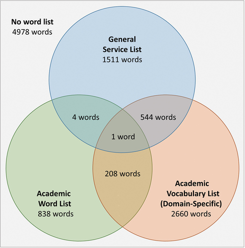
The entire process reduced the dataset from 407,510 unique letter strings to 10,744 words with complete data. We retained 2,060 (90.19%) basic, 1,051 (35.53%) general academic, 3,413 domain-specific (41.12%), and 4,978 words not present in any of the three samples; many words overlapped between samples (see Figure 1). For example, “medical” appears in all three samples, 774 words appear in at least two, and 5,267 appear in only one.

Figure 1. Overlap between word lists for unique words with complete data (n = 10,744 words).

Analyses

To determine the factor structure for word characteristics from different word samples (i.e., RQ1), we conducted separate maximum likelihood EFAs with each word sample as the reference. Each model factored the correlation matrix using only words with complete data from the relevant sample and maximum likelihood estimation of the factors, along with a direct oblimin rotation via the psych package for R (Revelle, 2020). The final models met multivariate assumptions, correlational matrix adequacy, and sampling adequacy. We computed factor scores for all words based on each model to address how different factor spaces compare (i.e., RQ2), then examined the distributions of factor scores for the different populations of words when scored according to the three different reference spaces.

Results

Table 2 includes descriptive information about word features from each sample, with features in alphabetical order and word lists moving from basic to discipline-specific. For example, the fifth row shows that the average length of basic words is 5.84 letters, but for general academic words is 8.57 and 7.31 for domain-specific words. The 16^th row shows that basic and general academic words are semantically dispersed (mean semd = 1.80 and 1.79, respectively), but domain-specific words are an entire standard deviation less dispersed (mean semd = 1.44, SD = 0.30).

Table 2. Descriptive statistics for word features by word list.

	General Service List (GSL)		Academic Word List (AWL)		Academic Vocabulary List – Domain Specific (AVL-DS)
	n = 2060		n = 1051		n = 3413
Word Feature	M	SD	M	SD	M	SD
cd	1036.52	2453.23	175.54	300.74	142.06	424.10
cocazipf	4.62	0.64	4.15	0.57	3.82	0.59
d	0.80	0.14	0.71	0.19	0.56	0.21
freqband	6.09	0.67	5.83	0.62	5.31	0.60
length	5.84	2.01	8.57	2.33	7.31	2.45
log_freq_hal	9.72	1.60	8.70	1.45	7.71	1.52
log_freq_kf	1.62	0.63	1.16	0.55	0.82	0.58
nmorph	1.32	0.58	2.19	0.83	1.73	0.78
nphon	4.75	1.81	7.40	2.15	6.19	2.27
nsyll	1.75	0.86	3.02	1.05	2.45	1.13
og_n	3.01	4.54	0.36	1.33	1.54	3.30
old	2.02	0.72	2.84	0.79	2.59	0.94
ortho_n	5.00	6.38	0.65	1.84	2.52	4.59
phono_n	11.87	14.39	1.39	4.31	5.84	10.59
pld	1.87	0.82	2.94	0.98	2.57	1.15
semd	1.80	0.27	1.79	0.25	1.44	0.30
subzipf	4.44	0.75	3.41	0.67	3.38	0.77
word_age	742.83	243.53	499.54	185.46	542.02	251.93
wordnet_lnapossam	1.73	0.82	1.26	0.68	1.09	0.79
wordsmyth_lnapossam	1.70	0.73	1.06	0.61	1.07	0.72
z_sem_prec	−0.03	0.73	−0.14	0.87	0.24	0.86
zenozipf	4.67	0.64	3.91	0.60	3.71	0.68

This table includes only the final 22 features used in the models.

RQ1.

Factor structure for GSL, AWL, and AVL-DS words

Model fit

We considered five methods for determining the number of factors for each word sample using the nFactors (Raiche, 2010) and psych (Revelle, 2020) packages in R, which consistently suggested four- or five-factor solutions, which we assessed for all samples (Table 3). We discuss the final solutions here.

Table 3. Factor analysis fit by word list reference.

	General Service List (GSL)	Academic Word List (AWL)	Academic Vocabulary List – Domain Specific (AVL-DS)
Bartlett’s test
df	231	231	231
X^2	50136.55	20743.13	72063.03
p	<.0001	<.0001	<.0001
Plot suggestions
Parallel Analysis (fa.parallel)	5	5	5
Parallel Analysis (nFactors)	4	5	4
Optimal Coordinates (nFactors)	4	5	4
Eigenvalues > Mean	5	5	4
Eigenvalues >1	5	5	4
Acceleration Factor	1	1	1
5-Factor Model Fit
% Variance Explained	75%	69%	68%
Overall Sampling Adequacy (MSA)	0.92	0.90	.92
Comparative Fit Index (CFI)	0.962	0.948	.956
Tucker-Lewis Index (TLI)	0.934	0.907	.923
Root Mean Square of Residuals (RMSR)	0.02	0.02	.03
Root Mean Square Error of Approximation (RMSEA)	0.083	0.088	.084
Lower Bound	0.080	0.084	.081
Upper Bound	0.087	0.093	.086
4-Factor Model Fit
% Variance Explained	71%	65%	67%
Overall Sampling Adequacy (MSA)	0.92	0.90	.92
Comparative Fit Index (CFI)	0.943	0.923	.933
Tucker-Lewis Index (TLI)	0.912	0.88	.896
Root Mean Square of Residuals (RMSR)	0.03	0.04	.03
Root Mean Square Error of Approximation (RMSEA)	0.096	0.010	.097
Lower Bound	0.093	0.096	.095
Upper Bound	0.099	0.105	.100

Higher values (at least above .90) indicate adequate model fit for MSA, CFI, and TLI. Lower values (at least below .10 indicate adequate model fit for RMSR and RMSEA.

For the GSL, the four-factor model fit was poor and combined the Frequency and Diversity factors, making the five-factor model preferable. The model had overall good fit, with the RMSEA indicating moderate fit (.083), the RMSR indicating excellent fit (.02), and the CFI and TLI also indicating excellent fit (.962 and .934, respectively; Table 3), and explained 75% of the variance in word features.

The four-factor model had poor fit and combined Frequency and Diversity factors for the AWL, also. The five-factor model had overall good fit, with the RMSEA indicating moderate fit (.088), the RMSR indicating excellent fit (.02), and the CFI and TLI also indicating excellent fit (.948 and .907, respectively;), and explained 69% of the variance.

For the AVL-DS, the five-factor model had good fit but contained a factor with pld alone. The four-factor model still had overall good fit, with the RMSEA indicating moderate fit (.092), the RMSR indicating excellent fit at (.03), and the CFI and TLI also indicating good fit (.933 and .896, respectively;), and explained 67% of the variance.

Factor loadings

Table 4 contains standardized factor loadings for the final model of each word list. Measures are in order of factor loadings on the GSL-reference model so that groupings are easier to see. For example, the COCA frequency had the strongest loading on the Frequency factor for all word lists. Table 4 also shows each factor’s explained variance, eigenvalue, and standardized α within the model for the specified word list.

Table 4. Factor loadings by Wordlist.

	Frequency			Complexity			Proximity			Polysemy (Polysemy/Diversity)^a			Diversity
	GSL	AWL	AVL-DS	GSL	AWL	AVL-DS	GSL	AWL	AVL-DS	GSL	AWL	AVL-DS	GSL	AWL
cocazipf	1.00	0.99	0.98	0.02	0.02	0.02	−0.01	0.01	0.01	0.01	−0.04	−0.03	−0.02	−0.02
log_freq_kf	0.96	0.86	0.83	0.08	0.07	0.09	0.00	0.00	−0.03	−0.01	0.03	0.06	0.03	0.06
zenozipf	0.95	0.89	0.84	−0.07	−0.01	−0.07	−0.01	0.01	0.02	0.02	0.02	−0.01	−0.06	0.06
log_freq_hal	0.90	0.89	0.84	0.02	−0.06	−0.03	0.02	0.00	0.02	0.06	0.02	0.03	0.04	−0.07
subzipf	0.84	0.73	0.77	−0.17	−0.11	−0.21	0.02	0.03	0.04	0.01	0.09	−0.02	−0.05	0.07
freqband	0.75	0.72	0.76	0.08	−0.07	0.10	−0.01	−0.08	−0.06	0.02	−0.01	−0.01	0.12	−0.07
cd	0.61	0.61	0.58	−0.06	0.04	0.05	0.09	0.12	0.07	−0.17	−0.02	0.01	0.15	0.04
wordage	0.30	0.29	0.29	0.06	0.06	0.02	0.00	−0.02	−0.02	0.11	0.16	0.29	0.16	0.32
nphon	−0.02	−0.02	−0.01	0.98	0.97	0.98	0.01	0.01	0.00	0.06	0.05	0.03	−0.01	0.01
nsyll	0.04	0.05	−0.01	0.90	0.84	0.90	0.02	−0.02	0.01	−0.06	−0.06	−0.03	0.01	−0.11
length	−0.05	−0.03	−0.01	0.89	0.97	0.94	−0.09	0.01	−0.05	0.03	0.07	0.07	−0.02	0.01
pld	0.03	0.02	0.00	0.87	0.86	0.88	−0.06	−0.02	0.00	−0.07	−0.08	−0.11	−0.02	0.00
nmorph	−0.07	−0.09	−0.02	0.78	0.69	0.77	0.16	0.04	0.08	−0.04	0.00	0.04	0.03	0.01
old	0.00	0.01	0.00	0.73	0.80	0.78	−0.22	−0.08	−0.11	−0.09	−0.12	−0.12	0.00	0.05
og_n	−0.01	0.01	−0.02	0.05	0.06	0.06	0.96	0.99	0.98	0.03	0.01	0.02	−0.02	0.00
ortho_n	0.03	0.00	0.02	−0.03	−0.02	−0.01	0.95	0.95	0.98	0.01	−0.01	−0.02	0.00	−0.01
phono_n	0.01	0.02	0.02	−0.27	−0.11	−0.17	0.64	0.78	0.73	0.01	−0.01	0.02	0.02	0.01
wordnet_lnapossam	0.00	−0.03	0.01	0.04	0.00	0.00	0.02	0.02	0.01	0.96	0.87	0.90	0.02	0.05
wordsmyth_lnapossam	0.05	0.10	0.03	−0.11	−0.08	−0.11	0.00	−0.02	0.04	0.79	0.68	0.70	0.00	−0.07
semd	0.00	0.01	0.24	−0.01	−0.01	0.06	−0.01	0.00	−0.01	0.01	0.05	0.39	0.98	0.74
d	0.27	0.33	0.52	0.03	−0.04	0.00	−0.01	0.00	−0.01	0.10	0.02	0.19	0.46	0.55
z_sem_prec	0.07	0.21	0.04	0.07	0.09	−0.14	0.04	0.02	0.00	0.03	0.24	−0.26	−0.42	−0.44
Explained Variance	26%	24%	24%	22%	21%	22%	12%	12%	12%	8%	7%	9%	7%	6%
Eigenvalue	5.65	5.24	5.21	4.91	4.65	4.93	2.55	2.58	2.62	1.77	1.49	1.93	1.59	1.31
Standardized Alpha	0.94	0.93	0.93	0.96	0.95	0.96	0.93	0.94	0.95	0.90	0.79	0.75	0.68	0.62

GSL – General Service List, AWL – Academic Word List, AVL-DS – Academic Vocabulary List (Domain-Specific). Loadings greater than .30 are bolded for ease.

^aFor the 4-factor solutions, results for the Polysemy-Diversity factor are reported under Polysemy.

For the GSL-reference model, the latent factor Frequency included all word frequency measures in the diverse corpora (the COCA, HAL, Educator’s Word Frequency Guide, Brown, Oxford English Dictionary, and Subtlex) with reasonably high loadings (from .99 for the COCA to .75 for the frequency band). However, Frequency also included contextual diversity and word age – albeit at lower loadings (.61 and .30, respectively). Frequency had a large eigenvalue (5.65), high reliability (α=.94), and explained 26% of the variance in word features.

For the AWL-reference model, Frequency also explained the most variance (24%, eigenvalue = 5.24) and was also highly reliable (α=.93). It included all word frequency measures in diverse corpora, with loadings ranging from .99 for the COCA to .61 for Subtlex-US. Two other measures loaded onto the Frequency factor: contextual diversity and dispersion, although relatively weakly (.61 to .32).

Frequency also explained the most variance for the discipline-specific-reference model (24%, eigenvalue = 5.21, α = .93). COCA frequency was again the highest-loading factor (0.98), followed by frequency in the Brown and HAL corpora, Educator’s Word Frequency Guide, and frequency band (0.76–0.84). The lowest loadings were for frequency based on the Subtlex corpus, contextual diversity, and dispersion (0.52–0.76).

The second latent factor, Complexity, measured various linguistic elements such as the number of letters, syllables, morphemes, and phonemes, as well as Levenshtein distances. It exhibited high loadings ranging from .98–.72, with phonemes and old20 having the highest and lowest loadings, respectively. Additionally, Complexity had a high eigenvalue and reliability coefficient (4.91; α = .96), explaining 22% of the variance. Similar results were observed for the AWL-reference model, with Complexity being a strong and reliable factor that explained 21% of the variance (eigenvalue = 4.65, α = .95). Letters and phonemes had the strongest loadings (.96 and .97, respectively), while the number of morphemes, syllables, and Levenshtein distances had relatively lower – but still strong – loadings (.69–.86). Similarly, Complexity explained 22% of the variance for the AVL-DS-reference model and was the most internally-stable factor (eigenvalue = 4.93, α = .96). The number of letters, syllables, and phonemes were the strongest loading measures (.90–.98), followed by phonologic Levenshtein distance (.88). Orthographic Levenshtein distance and the number of morphemes had weaker loadings at .77.

Factor 3, Proximity, included the size of orthographic, phonologic, and phonographic neighborhoods. This factor contained high loadings, ranging from .96–.64 (orthographic versus phonographic neighborhood, respectively) for the GSL-reference model. However, the reliability (α=.93), eigenvalue (2.55), and explained variance (12%) were lower than the previous two factors. Findings for both the AWL-reference and AVL-DS-reference models were similar: Proximity explained 12% of the variance in word characteristics and had a reliability of .94–.95, respectively. However, Proximity loadings were also high: .99 for phonographic, .95 for orthographic, and .78 for the phonologic neighborhood size, for the AWL; .98 for orthographic and phonographic, and .73 for the phonologic neighborhood for the AVL-DS.

Factor 4, Polysemy, included the two measures of senses and meanings from WordNet (loading=.96) and Wordsmyth (loading=.79). Even with only two items, this factor retained acceptable reliability (α=.90), while the eigenvalue (1.72) and explained variance (8%) were lower than previous factors. For the AWL-reference model, Polysemy also had reduced explained variance (7%, eigenvalue = 1.49) and reliability (α=.79). The loading for the number of senses and meanings from WordNet was stronger than the loading based on Wordsmyth (.87 and .68, respectively).

The latent factor Polysemy is a mix of polysemy and diversity measures for the discipline-specific model. Polysemy/Diversity explained the least amount of variance and was less reliable than previous factors (9%, eigenvalue = 1.93, α = .75). The number of senses and meanings from various dictionaries loaded strongest (WordNet and Wordsmyth, at .90 and .70, respectively), followed by a relatively weaker loading for semantic diversity (.39).

The GSL- and AWL-reference models included semantic dispersion and precision as Diversity. Loadings were more varied on this factor (0.98 for semantic dispersion to − 0.42 for semantic precision), and the eigenvalue (1.59), explained variance (7%), and reliability (α=.68) were considerably lower than for other factors on the GSL-reference model. For the AWL-reference model, Diversity and Polysemy explained a similar amount of variance (6% vs. 7%, eigenvalue = 1.31) but with lower reliability (α=.62 vs. .79); and included semantic diversity, precision, and word age, along with the cross-loaded dispersion.

RQ2.

Comparison of factor spaces

To compare the different factor spaces to one another, we examined the correlations among factors and the distributions of factor scores by scoring the words in each reference sample using the factor score regressions from the three separate analyses. To examine factor correlations and densities, we present scatterplot matrices in Figures 2–4 for GSL-, AWL-, and AVL-DS-reference models. For example, Figure 2 is based on the model created by analyzing only GSL words but includes red plots for estimated factor scores on AVL-DS words based on the GSL-reference model. Figure 2 plots density curves for each word sample on the diagonal, along with the factor correlation above the diagonal and a scatterplot below the diagonal. Across Figures 2–4, red plots consistently show the estimated factor scores for AVL-DS words, green plots show AWL words, blue plots show GSL words, and purple plots show all words in any list. These estimates change across figures because the scoring coefficients differ depending on the reference sample used in the analysis. See Table 5 for a set of example words and their factor score estimates in each model.

Figure 2. Factor correlations for the GSL-reference model estimated on each word sample. Note: Scatterplots below the diagonal contain random 200-word samples while density plots and correlations on and above the diagonal are based on entire word samples. Word samples include AVL_DS (red) Academic Vocabulary List Domain-Specific; AWL (green) Academic Word List; GSL (blue) General Service List; Words (purple) in any word list.

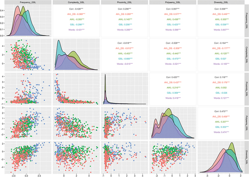
Figure 3. Factor correlations for the AWL-reference model estimated on each word sample. Note: Scatterplots below the diagonal contain random 200-word samples while density plots and correlations on and above the diagonal are based on entire word samples. Word samples include AVL_DS (red) Academic Vocabulary List Domain-Specific; AWL (green) Academic Word List; GSL (blue) General Service List; Words (purple) in any word list.

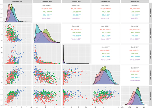
Figure 4. Factor correlations for the AVLDS-reference model estimated on each word sample. Note: Scatterplots below the diagonal contain random 200-word samples while density plots and correlations on and above the diagonal are based on entire word samples. Word samples include AVL_DS (red) Academic Vocabulary List Domain-Specific; AWL (green) Academic Word List; GSL (blue) General Service List; Words (purple) in any word list.

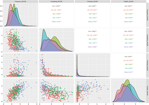
Table 5. Example words and factor estimates based on each model.

		GSL (General Service List) Reference Model					AWL (Academic Word List) Reference Model					AVLDS (Domain-Specific Word) Reference Model
word	Word List	Frequency	Complexity	Proximity	Polysemy	Diversity	Freq	Comp	Prox	Poly	Div	Freq	Comp	Prox	Poly-Div
accept	GSL	0.41	0.49	−0.64	0.66	1.04	1.47	−0.89	−0.07	1.52	1.12	2.04	−0.22	−0.38	1.62
honest	GSL	−0.05	0.09	−0.75	0.15	0.22	0.93	−1.16	−0.27	0.92	0.81	1.48	−0.53	−0.53	1.11
jaw	GSL	−0.88	−1.08	1.91	0.07	−1.21	−0.10	−2.31	8.36	0.86	−0.78	0.46	−1.56	3.15	0.89
library	GSL	0.34	1.18	−0.78	−0.43	−1.66	1.42	−0.27	−0.31	0.25	−0.36	1.86	0.31	−0.56	0.37
meet	GSL	0.91	−0.91	0.41	0.98	1.34	2.09	−2.13	3.89	1.93	1.45	2.62	−1.36	1.08	1.97
nice	GSL	0.68	−0.93	0.68	0.17	−0.60	1.82	−2.08	4.83	1.03	−0.30	2.27	−1.36	1.44	1.08
race	GSL	0.65	−1.05	1.68	0.92	−1.13	1.69	−2.22	8.42	1.86	−0.44	2.18	−1.44	2.80	1.89
size	GSL	0.91	−0.96	0.09	0.63	1.01	2.18	−2.15	3.10	1.51	1.17	2.62	−1.38	0.61	1.68
usual	GSL	0.32	0.39	−0.77	−1.12	1.22	1.33	−0.94	−0.28	−0.57	1.61	1.81	−0.29	−0.55	0.00
wood	GSL	0.30	−0.89	0.93	0.52	−0.44	1.43	−2.08	4.96	1.43	−0.02	1.86	−1.34	1.84	1.40
abandon	AWL	−0.82	0.99	−0.77	0.16	1.06	−0.01	−0.42	−0.31	0.97	0.50	0.62	0.18	−0.54	1.09
compile	AWL	−1.97	0.55	−0.70	−0.74	0.03	−1.17	−0.77	−0.28	−0.16	−0.62	−0.51	−0.17	−0.52	0.11
evidence	AWL	0.93	1.22	−0.77	0.04	0.70	2.02	−0.22	−0.30	0.89	0.84	2.55	0.34	−0.57	1.07
illustrate	AWL	−0.82	1.85	−0.77	−0.82	0.49	0.01	0.39	−0.32	−0.14	0.74	0.58	0.84	−0.57	0.24
maximize	AWL	−1.53	1.46	−0.71	−1.46	−0.73	−0.82	0.03	−0.32	−1.00	−0.87	−0.13	0.58	−0.55	−0.57
nonetheless	AWL	−0.74	2.65	−0.82	−2.24	0.96	−0.03	1.02	−0.35	−1.86	1.17	0.60	1.35	−0.60	−1.06
process	AWL	1.18	0.56	−0.55	0.97	0.89	2.41	−0.78	0.13	1.91	1.12	2.92	−0.15	−0.23	1.97
ratio	AWL	−0.39	0.20	−0.43	−1.26	−0.52	0.47	−1.11	0.54	−0.71	−0.33	0.98	−0.47	−0.16	−0.32
significant	AWL	0.60	3.10	−0.77	−0.71	1.34	1.50	1.36	−0.34	−0.09	1.37	2.14	1.84	−0.60	0.45
underlying	AWL	−0.62	1.88	−0.71	−0.26	0.59	0.16	0.38	−0.32	0.47	0.46	0.81	0.87	−0.55	0.85
absenteeism	AVLDS	−2.76	3.53	−0.76	−2.59	−1.44	−2.23	1.68	−0.38	−2.25	−1.58	−1.51	1.99	−0.58	−1.68
autopsy	AVLDS	−1.85	0.89	−0.76	−1.44	−2.14	−1.19	−0.47	−0.30	−0.95	−2.18	−0.49	0.07	−0.55	−0.69
carbon	AVLDS	−0.19	0.13	−0.42	−0.49	−2.29	0.84	−1.06	0.36	0.23	−1.50	1.26	−0.41	−0.06	0.31
habitable	AVLDS	−2.47	1.74	−0.68	−2.18	−1.47	−1.91	0.32	−0.31	−1.76	−1.03	−1.32	0.78	−0.53	−1.16
membrane	AVLDS	−1.25	1.21	−0.80	−1.37	−2.50	−0.33	−0.13	−0.31	−0.79	−1.63	0.12	0.36	−0.57	−0.65
linguistic	AVLDS	−1.27	2.50	−0.74	−1.55	−2.86	−0.57	0.93	−0.35	−1.09	−1.49	0.08	1.40	−0.58	−0.65
positivism	AVLDS	−2.86	2.90	−0.56	−1.81	−3.68	−2.34	1.21	−0.16	−1.36	−3.16	−1.69	1.67	−0.39	−1.03
sacrificial	AVLDS	−2.37	2.88	−0.75	−2.36	−2.01	−1.79	1.22	−0.36	−1.98	−1.86	−1.12	1.58	−0.57	−1.41
tuberculosis	AVLDS	−1.50	4.60	−0.89	−2.51	−1.72	−0.76	2.58	−0.43	−2.06	−0.87	−0.26	2.85	−0.63	−1.73
wavelength	AVLDS	−1.75	2.04	−0.86	−1.61	−2.43	−0.97	0.53	−0.35	−1.04	−2.70	−0.44	0.89	−0.59	−0.93

Bolded estimates indicate when words were part of the sample used to create that model. Not bolded estimates were estimated separately, after creating models.

For brevity, Freq – Frequency, Comp – Complexity, Prox – Proximity, Poly – Polysemy, Div – Diversity, and Poly-Div – Polysemy/Diversity factors.

Correlations between factors

In the GSL-reference model, significant correlations (p < .001) were observed among factors, as shown in Figure 2. The strongest negative correlation was between Complexity and Proximity (−.67), indicating that more complex words had fewer neighboring words. Frequency and Diversity were positively correlated at .54, suggesting that frequently used words appear in various contexts. The mid-range correlations (ranging from − .47 to .41) were all related to Polysemy, indicating that more complex words tend to have fewer meanings and that words with more meanings tend to be used more frequently and have more neighbors. Polysemy and Diversity had a weak but still significant correlation at .30. Frequency showed the weakest correlations, with Complexity being negatively correlated at − .28 and Proximity positively correlated at .20.

Comparing the estimated correlations using the AWL and AVL-DS words and the GSL-reference model, there are a few apparent differences across reference word lists. The most striking finding is that the estimated correlations among factors are generally larger when based on all words across all lists, except for the correlation between Proximity and Complexity. The next striking finding is that correlations are usually somewhat weaker when calculated from AWL-sample estimates compared to GSL-sample or AVL-DS-sample estimates against the GSL-reference model.

Similar to the GSL-reference model, nearly all correlations between factors were significant at p < .001 for the AWL-reference model (Figure 3). Complexity and Proximity again correlated the strongest (−.48), indicating that less complex words tend to have more words in their neighborhood. Frequency and Polysemy then correlated moderately at .47, indicating that words used more frequently have more meanings. Frequency also correlated moderately with Diversity (.45) and with Complexity (−.39). Polysemy correlated moderately with Complexity (−.42) and weakly with Proximity (.25). The weakest correlations included Frequency and Proximity (.21), Diversity and Polysemy (.20), and Diversity with Complexity (−.16). Our previous observation that correlation estimates based on the AWL sample tend to be somewhat weaker than GSL- and AVL-DS-sample estimates mostly hold for the AWL-reference model.

For the AVL-DS-reference model, all correlations between factors were significant at p < .001 (Figure 4). Frequency and Polysemy/Diversity correlated the strongest, closely followed by Complexity and Proximity (.63 and − .62, respectively). The Polysemy/Diversity factor then correlated moderately with Complexity and Proximity (−.47 and .45, respectively). The weakest correlations were still quite strong for Frequency with Proximity and Frequency with Complexity (.39 and − .36, respectively). Comparing the estimates for different word lists using the AVL-DS-reference, we again see that correlations are somewhat weaker for the AWL-sample estimates and tend to be strongest for the entire word sample estimates. The consistency of the latter finding across all three scoring models suggests that the three specific word lists somewhat restrict the range of observations, such that when the restriction of range is removed, correlations are stronger.

Comparing the correlations across the separate analyses reveals the correlations were reasonably consistent. Although exploratory and descriptive, these comparisons are consistent with the notion that the estimated factors are the same, regardless of which word list is the reference. That is, the characteristics of words seem to define a common set of dimensions regardless of the reference word list used to define the space. What changes between analyses is the reference space and the distribution of factor scores within that reference space, but not the factors themselves.

Comparing factor score estimates across models and samples

As mentioned above, we estimated factor scores for each word sample (and all word samples together) based on separate models for each target population. Thus, Figures 2–4 also compare the factor score distributions in the different reference word lists and across all words. For example, we can see from the density plots for Frequency in Figure 2 that general academic words (AWL) are less frequent because the green Frequency density plot is further to the left than the blue (GSL). The same holds for the density plots in Figures 3 and 4, where general academic words (AWL) and domain-specific words (AVL-DS) serve as the model reference.

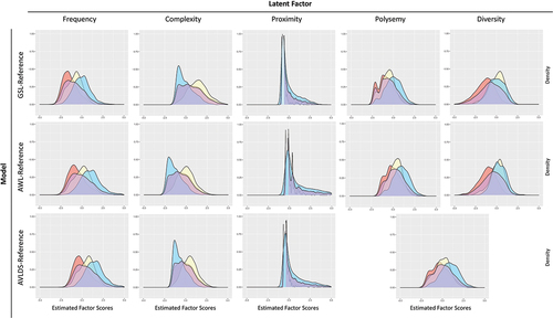
Figure 5 displays scaled density plots for each factor across the three scoring models and four word samples (GSL, AWL, AVL-DS, All Words). Each row represents one scoring model, while each column is the density plot for a specific factor. The color of the density plot still indexes the word sample used for estimation. Hence, the first row uses the GSL-reference model to estimate factor scores, while the first column shows the distribution of the Frequency factor across all three reference models. Thus, the first cell shows the distribution of scores for the Frequency factor using the GSL-reference model. The least frequent words are the domain-specific words (red), then general academic words (green), and finally, basic words (blue), with the entire range represented in purple. The choice of reference model has a negligible impact on the factor distribution; what matters is which word sample is used to estimate the distribution. We reach the same conclusions regardless of model examined, except for Polysemy/Diversity, which is one factor in the AVL-DS scoring model and separate factors in the GSL and AWL models. We host animations of the scaled density plots to demonstrate how the different samples of words compare across various models at https://academicvocab.times.uh.edu/. These animations show more clearly the slight variations induced by shifting the reference distribution for a factor as the scoring model shifts from one reference sample to another.

Figure 5. Scaled density plots by reference model and latent factor. Note: Word list samples are: GSL (blue) General Service List; AWL (yellow) Academic Word List; AVLDS (red) Academic Vocabulary List Domain-Specific; Words (purple) in any word list.

Discussion

To some extent, learners’ language contexts define the skills they need to develop and the opportunities to do so. Yet, few studies systematically parameterize the latent features of the diverse language environments that learners experience. This study focused on words as one critical language unit and asked what exploratory factor structures emerge for a systematic collection of word features and how those structures differ across purposely selected word lists. We searched the literature for empirical measures of words and included non-behavioral measures after 1950 for more than 1,000 words. We combined all the word features into a large dataset of 22 measures and 10,744 unique words with complete data and conducted analyses on data from three different word lists. We found that English word features grouped into a similar five-factor structure regardless of word list: Frequency, Complexity, Proximity, Polysemy, and Diversity, although the emerging factor structure for domain-specific words combined Polysemy and Diversity into a single factor. While we cannot explicitly test the equivalence of factor structures using the current exploratory factor analytic methods, we were able to compare our three models descriptively. The differences between factor structures were minor, suggesting that word features identify the same latent dimensions regardless of the reference word list. Below we discuss the similarities and differences in the factor structures, the implications for this work, and its limitations.

Comparing models with different reference samples

Analyses revealed some factors were stable in all models while others were less so.

Universal word factors

Frequency

The latent Frequency construct describes a word’s occurrence rate and is considered a proxy for relative exposure level; words that are more frequent in text and speech are more likely to be encountered more often. Since encounters with words provide opportunities to learn them, it is unsurprising that frequency has been a significant predictor of which words children know (Goodman et al., 2008; Swanborn & De Glopper, 1999), the efficiency with which learners process words (Brysbaert et al., 2018; Monsell et al., 1989), and how well learners know a word (Ellis, 2002).

The obtained Frequency factor in our study includes all word frequency measures for each reference model. Corpus frequency measures are highly correlated (Breland, 1996), and all estimate how frequently a word is used by counting occurrences in corpora from different sources. Our latent factor incorporates frequency scores from various corpora and is thus more representative than a frequency measure derived from any single corpus. As a result, researchers not interested in word frequency in specific modalities or formats may wish to use our factor scores that account for word frequency across modalities and corpora.

The Frequency factor also includes a few measures that do not directly measure raw frequency in a corpus: contextual diversity, dispersion, and word age. That being said, contextual diversity and dispersion do measure frequency at a larger grain size. Adelman et al. (2006) operationalize contextual diversity as the number of documents in which a word appears in a corpus. Zeno et al. (1995) operationalize dispersion as the number of content areas in which a word appears in a corpus. Thus, both are corpus-derived frequency measures, and our results suggest that these measures reflect a latent Frequency dimension. Researchers intending to control for frequency effects might want to consider using our latent score that accounts for these related measures rather than only raw frequency measures.

Raw frequency from the Corpus of Contemporary Academic English (COCA) was the strongest-loading measure on our latent Frequency factor. We had expected that frequency measures based on conversational corpora (e.g., Subtlex) would be stronger for basic words. However, the COCA contains almost ten times as many words as Subtlex; our results highlight the large corpora’s dominating utility.

Complexity

The obtained Complexity factor relates to the orthographic and phonological difficulty of a word, which relates to the ease or difficulty of learning to say (Ehri, 2014), read (Carlisle, 2000), or process (Ehri, 2005) a word. Words that take longer to process or are difficult to decode tend to make reading more challenging (Carlisle, 2000; Ehri, 1992). On the other hand, information theory supports that longer words are more likely to contain more meaningful information than shorter words (Mahowald et al., 2013; Piantadosi et al., 2011). For example, “unbreakable” has three pieces of information: “un-break-able,” making it a denser and abstract word than “break” alone. The measures that load on the Complexity factor describe these different but related ways a word could be challenging to decode, encode, and process. For example, a word can be difficult to process due to a complex orthography or phonology, but these do not correlate perfectly (e.g., “cough”).

Levenshtein distances also loaded onto the Complexity factor. We expected these to load onto Proximity, yet, scores on neighborhood sizes (the Proximity factor) and Levenshtein distances vary systematically but not linearly. For example, words with a score of one on the old20 measure can have anywhere between 11–35 close neighbors (words that are exactly one change away from the original word). Furthermore, there is a considerable variation in neighborhood size when Levenshtein distances are small but minimal variation when Levenshtein distances are large. Thus, it is unsurprising that other researchers found the Levenshtein distances to load onto Complexity.

Measures on Complexity are fixed-analytic computations and corpus-free (i.e., the number of letters or syllables in a word is the same regardless of where you read it, with dialectic exceptions). Our latent Complexity factor gives researchers a measure of orthographic and phonological complexity that accounts for information from related measures while mitigating concerns about multicollinearity.

Proximity

The latent Proximity construct measures how many words are closely related to this word visually and aurally. Words in dense neighborhoods tend to be learned earlier, especially as we engage in phonological awareness training at a relatively young age. We recognize words with many neighbors more quickly, although which type of neighborhood (phonological or orthographical) is most useful is still debated (Adelman & Brown, 2007). Further, neighborhood size could be the driving factor behind the word length effect on recall (Jalbert et al., 2011).

The Proximity factor included measurements of neighborhood size. The phonographic neighbors were consistently the strongest-loading measure. The clear distinction of the Proximity factor from other factors stems from the shape of the distributions of the three measures of neighborhood size. These distributions are highly positively skewed, with a large concentration around zero. Many multi-syllable words cannot transpose into any other word with only one change, such as “straightforward,” while few words reside in large neighborhoods, such as “cat,” with 32 phonologic neighbors. Similar to Complexity, Proximity contains distinct but highly related measures. Consequently, using the factor scores broadly represents a word’s proximity to other words while mitigating concerns about multicollinearity from using multiple measures.

Consistent word factors

The remaining two factors were distinct and weakly correlated for the basic- and general academic-reference models but combined into a single factor for the domain-specific model. We label these factors consistent as they were similarly defined across the different reference spaces, although consolidated into a single dimension for domain-specific words.

Polysemy

The latent Polysemy construct relates to how many distinct meanings and related senses a word has. Polysemy is an essential feature of all languages and there seem to be similarities in how different languages extend the senses of words to related concepts (Youn et al., 2016). Words with many related senses are processed more efficiently (Azuma & Van Orden, 1997; Borowsky & Masson, 1996; Hino & Lupker, 1996); second language learners may not enjoy the same advantages in learning polysemous words as their peers do. Some words have alternative senses that can be used in a wide variety of documents or contexts (“grasp” a cup or “grasp” an idea). Other words have senses that are more constrained by the document or disciplinary genre (jail “cell” versus biological “cell.”)

Diversity

The latent Diversity construct describes the number of contexts in which a word can be used and encompasses global and local contexts. The global context is at the discipline or document level, such as contextual diversity, which counts the number of documents among a large corpus in which a word occurs. When a word is used in more documents or contexts, it may provide more learning opportunities, which explains why the contextual diversity measure explains lexical processing efficiency so well (Adelman et al., 2006; Jones et al., 2012). At a more global level, the documents that include a word can be categorized by academic discipline resulting in a variable called dispersion (Zeno et al., 1995). Our latent factor accounts for both these measures and a measure of diversity at the sentence (local) level. Semantic diversity considers the words used next to or near a target word across documents in a corpus. The relationship between Diversity and Polysemy is easy to understand when considering that a word with more meanings can usefully be employed in more diverse contexts. Semantic precision also relates to diversity (negatively) as it describes how far down a word is down a hypernym chain (Fellbaum, 2005).

Considerations for domain-specific words

Findings were slightly different for domain-specific words. The criterion used to identify domain-specific words ensured that these words are used in a limited number of contexts. As document-level variability for domain-specific words is constrained, so is the utility of global diversity measures such as contextual diversity or dispersion, which measure use across documents and disciplines. Conversely, word features that measure local variability relate to the number of senses and meanings a word has and thus loads onto the Polysemy/Diversity factor, as shown in Table 3. Instead of one factor for global/local diversity and one for polysemy, we also found that global diversity measures loaded with Frequency, and the local diversity measure loaded with Polysemy in the analysis of domain-specific words. Given these constraints, it is sensible that global diversity measures are related to the overall frequency of the word, as we see in Table 3: dispersion and contextual diversity load onto the Frequency factor.

Factor correlations

Our models used oblique rotations so that factors could correlate if appropriate. The correlations between factors generally followed the same direction and level of statistical significance for all models. However, the magnitude varied somewhat across word lists, possibly partly due to sampling variability and parameter differences. Complex words consistently had fewer neighbors; frequent words were used more diversely and had more senses and meanings, regardless of word set. Diverse words had little relation with neighborhood size or complexity.

The correlation pattern between the basic and general academic word models was similar (Figures 2 and 3). Nearly all factors correlated statistically significantly at p < .001, suggesting that the oblique rotation was necessary. Moreover, magnitudes ranged from .16 to .67, emphasizing that selecting five factors was suitable.

The relationships between factors remained stable across reference models, despite domain-specific words collapsing into four factors. One notable difference was a nonsignificant relationship between Diversity and Complexity for basic words, although still positive. This may be because the words sampled for basic words are less complex than the general academic and domain-specific words. Proximity and Complexity also correlated more weakly for general academic words than for others.

Still, the stability of the relationships between factors across models is noteworthy. For example, the correlation between Proximity and Complexity is consistently either the strongest or second strongest correlation. The correlation between Frequency and the Polysemy/Diversity combination was the other strongest correlation for all domain-specific models; however, correlations of Frequency with separate Polysemy and Diversity were moderate for both basic- and academic-reference models.

Previous data-driven models

Our work advances the field beyond previous studies in two ways. First, we included words from all parts of speech. Secondly, we excluded measures based on human ratings and behaviors. Third, our statistical models allowed factors to correlate, thereby reducing mathematical constraints that are not driven by linguistic data. Despite these differences, our findings were generally similar to those of prior authors. For example, Clark and Paivio’s (2004) model with 925 nouns also shows word frequency measures loading onto a Frequency factor and the number of letters and syllables loading onto a Complexity-like factor. Although Clark and Paivio (2004) restricted the models to uncorrelated factors, they acknowledged the issue of cross-loading, “implicating a multi-dimensional underlying structure for these variables” (p. 376). Similarly, Yap et al. (2012) used principal components analysis on ten measures included in our models. In this analysis, the Length and Neighborhood components are identical to our Complexity and Proximity factors, while the Frequency/Semantic component contained one measure from our Frequency, Polysemy, and Diversity factors each.

Brysbaert et al. (2019) model is arguably most aligned with our models. This model included the most measures in our model and an oblique rotation. We found this change of particular importance, as the individual measures are not necessarily highly correlated because they measure a similar construct, but because the constructs themselves are strongly related. Brysbaert et al. (2019) identified similar Frequency and Complexity-like factors, with variables loading according to our model’s factor pattern – including contextual diversity onto Frequency. The main difference is that the orthographic and phonologic Levenshtein distances for the 20 closest neighbors (old20 and pld20) loaded onto both the Complexity and Proximity factors, unlike our models and Yap et al. (2012) model, where old20 and pld20 only loaded onto Complexity. However, it is worth noting that old20, pld20, and neighborhood density measures would have cross-loaded onto Complexity and Proximity in Yap et al. (2012) model if they had used a .30 cutoff for factor loadings, as in Brysbaert et al. and the current study. Paivio’s (1968) and Clark and Paivio’s (2004) models do not include old20, pld20, or any neighbor measures. Brysbaert et al. (2019) also found a similar pattern to our correlation matrix for general academic words.

Limitations

The study has important limitations. First, though conceptually different, the three word lists used in this study are not completely distinct at the word level, and alternatives could have been used. We believe the consistency of findings across these lists suggests that these results will generalize to other lists representing more specialized contexts. It would be particularly interesting to see if these findings replicate with lists of words used frequently in child directed speech. Second, although the present study includes many word features, future research will produce additional measures.

Research applications

The current study indicated that five main latent factors underlie the empirical non-behavioral lexical measures, namely, Frequency, Complexity, Proximity, Polysemy, and Diversity, that may prove useful to understand how learners learn new words, select equivalent words for assessment or stimuli, or statistically control for differences in said stimuli. For example, Lawrence et al. (2022) used these five latent factors to explore interactions between lexical characteristics and reading performance.⁸ In their study, factor scores obviated the need to make difficult decisions about specific measures to include while still accounting for the maximum effects of word characteristics on item difficulty. Future research can also use latent factor scores to identify sets of matched words when designing innovative intervention studies or vocabulary knowledge measures, for example, matching on Frequency as a holistic dimension, as opposed to a single corpus frequency measure.

Disclosure statement

No potential conflict of interest was reported by the author(s).

Additional information

Funding

This research was supported by the grant No. R305A170151 Improving the Accuracy of Academic Vocabulary Assessment for English Language Learners, grant No. R305A090555 Word Generation an Efficacy Trial, and grant No. R305A080647 Measuring the Development of Vocabulary and Word Learning to Support Content Area Reading and Learning from the Institute of Educational Sciences.

Notes

1. Using the raw frequency can be problematic in model estimation because of Zipf’s law: the frequency of a word is inversely proportional to its ranking. A few high-ranking words take up a significant portion of corpora (e.g. “the,” “and,” “a”), many low-ranking words take up a small portion of corpora (e.g. “projectile,” “calendar”), and frequency and rankings are not linearly related. For this reason, linear models tend to instead be based on some transformation of the raw frequency – either a log transformation or zipfian transformation. The zipfian transformation accounts for the word frequency effect based on Zipf’s law (Van Heuven et al., 2014) and is calculated as: $\mathit{lo}{g}_{10}(\frac{\mathit{raw}\mathit{frequency}+1}{\mathit{corpus}\mathit{size}\mathit{in}\mathit{millions}+\mathit{word}\mathit{types}\mathit{in}\mathit{millions}})+3$

2. Because the COCA splits by part of speech, we totaled word frequency for all parts of speech before taking the Zipfian transformation.

3. Because the OED is split by part of speech, we used the highest occurring frequency band for each word.

4. Neighborhood sizes were collected from the English Lexicon Project (Yap et al., 2012), however, no specific corpus is disclosed.

5. Because Ngram data splits by part of speech, we used the oldest occurrence for word age.

6. Because WordNet splits by part of speech, we took the average score for each word.

7. Other measures were considered for the factor analysis, but were too highly correlated with other measures (r > .98; Standardized Frequency Index (SFI) from Subtlex with zenozipf, and Contextual Diversity and Word Frequency from Subtlex with subzipf) or did not have enough variability to warrant inclusion for any word set (MSA < .60; mean bigram from English Lexicon Project and word age from Oxford English Dictionary).

8. This paper uses the general academic word (AWL-reference) model to estimate factor scores on a specific set of vocabulary from the Word Generation trials. Factor score estimates for these words differ in the current paper when the words are scaled based on the GSL-reference, AWL-reference, and AVL-DS-reference as opposed to scaled amongst themselves.

References

- Adelman, J. S., & Brown, G. D. (2007). Phonographic neighbors, not orthographic neighbors, determine word naming latencies. Psychonomic Bulletin & Review, 14(3), 455–459. https://doi.org/10.3758/BF03194088
- Adelman, J. S., Brown, G. D. A., & Quesada, J. F. (2006). Contextual diversity, not word frequency, determines word-naming and lexical decision times. Psychological Science, 17(9), 814–823. https://doi.org/10.1111/j.1467-9280.2006.01787.x
- Anglin, J. M., Miller, G. A., & Wakefield, P. C. (1993). Vocabulary development: A morphological analysis. Monographs of the Society for Research in Child Development, 58(10), i–186. https://doi.org/10.2307/1166112
- Azuma, T., & Van Orden, G. C. (1997). Why SAFE is better than FAST: The relatedness of a word’s meanings affects lexical decision times. Journal of Memory and Language, 36(4), 484–504. https://doi.org/10.1006/jmla.1997.2502
- Balota, D. A., Yap, M. J., Hutchison, K. A., Cortese, M. J., Kessler, B., Loftis, B., Neely, J. H., Nelson, D. L., Simpson, G. B., & Treiman, R. (2007). The English lexicon project. Behavior Research Methods, 39(3), 445–459. https://doi.org/10.3758/BF03193014
- Bates, E., Bretherton, I., & Snyder, L. S. (1991). From first words to grammar: Individual differences and dissociable mechanisms (Vol. 20). Cambridge University Press.
- Beck, I. L., McKeown, M. G., & Kucan, L. (2002). Bringing words to life: Robust vocabulary instruction. Guilford Press.
- Beretta, A., Fiorentine, R., & Poeppel, D. (2005). The effects of homonymy and polysemy on lexical access: An MEG study. Brain Research: Cognitive Brain Research, 24(1), 57–65. https://doi.org/10.1016/j.cogbrainres.2004.12.006
- Bhattacharya, A., & Ehri, L. C. (2004). Graphosyllabic analysis helps adolescent struggling readers read and spell words. Journal of Learning Disabilities, 37(4), 331. https://doi.org/10.1177/00222194040370040501
- Biemiller, A., & Slonim, N. (2001). Estimating root word vocabulary growth in normative and advantaged populations: Evidence for a common sequence of vocabulary acquisition. Journal of Educational Psychology, 93(3), 498–520. https://doi.org/10.1037/0022-0663.93.3.498
- Borowsky, R., & Masson, M. E. (1996). Semantic ambiguity effects in word identification. Journal of Experimental Psychology: Learning, Memory, and Cognition, 22(1), 63–85. https://doi.org/10.1037/0278-7393.22.1.63
- Breland, H. M. (1996). Word frequency and word difficulty: A comparison of counts in four corpora. Psychological Science, 7(2), 96–99. https://doi.org/10.1111/j.1467-9280.1996.tb00336.x
- Bryant, P., & Goswami, U. (1987). Beyond grapheme-phoneme correspondence. Cahiers de Psychologie Cognitive/Current Psychology of Cognition, 7(5), 439–443.
- Brysbaert, M., Mandera, P., & Keuleers, E. (2018). The word frequency effect in word processing: An updated review. Current Directions in Psychological Science, 27(1), 45–50. https://doi.org/10.1177/0963721417727521
- Brysbaert, M., Mandera, P., McCormick, S. F., & Keuleers, E. (2019). Word prevalence norms for 62,000 English Lemmas. Behavior Research Methods, 51(2), 467–479. https://doi.org/10.3758/s13428-018-1077-9
- Brysbaert, M., & New, B. (2009). Moving beyond Kučera and Francis: A critical evaluation of current word frequency norms and the introduction of a new and improved word frequency measure for American English. Behavior Research Methods, 41(4), 977–990. https://doi.org/10.3758/BRM.41.4.977
- Carlisle, J. F. (2000). Awareness of the structure and meaning of morphologically complex words: Impact on reading. Reading and Writing, 12(3), 169–190. https://doi.org/10.1023/A:1008131926604
- Cervetti, G. N., Hiebert, E. H., Pearson, P. D., & McClung, N. A. (2015). Factors that influence the difficulty of science words. Journal of Literacy Research, 47(2), 153–185. https://doi.org/10.1177/1086296X15615363
- Clark, J. M., & Paivio, A. (2004). Extensions of the Paivio, Yuille, and Madigan (1968) norms. Behavior Research Methods, Instruments, & Computers, 36(3), 371–383. https://doi.org/10.3758/BF03195584
- Coxhead, A. (2000). A new academic word list. TESOL Quarterly, 34(2), 213–238. https://doi.org/10.2307/3587951
- Dale, E., & O’Rourke, J. (1981). The living word vocabulary. World Book/Childcraft International.
- Davies, M. (2008). The corpus of contemporary American English (COCA): One billion million words, 1990-2019. https://www.english-corpora.org/coca
- DeRocher, J. (1973). The counting of words: a review of the history, techniques and theory of word counts with annotated bibliography. Syracuse University Research Corporation.
- Ehri, L. C. (1992). Reconceptualizing the development of sight word reading and its relationship to recoding. In P. B. Gough, L. C. Ehri, & R. Treiman (Eds.), Reading acquisition (pp. 107–143). Lawrence Erlbaum Associates, Inc.
- Ehri, L. C. (2005). Learning to read words: Theory, findings, and issues. Scientific Studies of Reading, 9(2), 167–188. https://doi.org/10.1207/s1532799xssr0902_4
- Ehri, L. C. (2014). Orthographic mapping in the acquisition of sight word reading, spelling memory, and vocabulary learning. Scientific Studies of Reading, 18(1), 5–21. https://doi.org/10.1080/10888438.2013.819356
- Ellis, N. C. (2002). Frequency effects in language processing: A review with implications for theories of implicit and explicit language acquisition. Studies in Second Language Acquisition, 24(2), 143–188. https://doi.org/10.1017/S0272263102002024
- Fellbaum, C. (2005). WordNet and wordnets. https://doi.org/10.1016/B0-08-044854-2/00946-9.
- Fenson, L., Dale, P., Reznick, J. S., Bates, E., Thal, D., & Pethick, S. (1994). Variability in early communicative development. Monographs for the Society for Research in Child Development, 59(5), i. https://doi.org/10.2307/1166093
- Field, A. (2013). Discovering statistics using IBM SPSS statistics. Sage Publishing.
- Gardner, D., & Davies, M. (2014). A new academic vocabulary list. Applied Linguistics, 35(3), 305–327. https://doi.org/10.1093/applin/amt015
- Goldfield, B. A., & Reznick, J. S. (1990). Early lexical acquisition: Rate, content, and the vocabulary spurt. Journal of Child Language, 17(1), 171–183. https://doi.org/10.1017/S0305000900013167
- Goodman, J. C., Dale, P. S., & Li, P. (2008). Does frequency count? Parental input and the acquisition of vocabulary. Journal of Child Language, 35(3), 515–531. https://doi.org/10.1017/S0305000907008641
- Hiebert, E. H., & Fisher, C. W. (2005). A review of the national reading panel’s studies on fluency: The role of text. The Elementary School Journal, 105(5), 443–460. https://doi.org/10.1086/431888
- Hiebert, E. H., Goodwin, A. P., & Cervetti, G. N. (2018). Core vocabulary: Its morphological content and presence in exemplar texts. Reading Research Quarterly, 53(1), 29–49. https://doi.org/10.1002/rrq.183
- Hino, Y., & Lupker, S. J. (1996). Effects of polysemy in lexical decision and naming: AN alternative to lexical access accounts. Journal of Experimental Psychology: Human Perception and Performance, 22(6), 1331–1356. https://doi.org/10.1037/0096-1523.22.6.1331
- Hino, Y., Lupker, S. J., & Pexman, P. M. (2002). Ambiguity and synonymy effects in lexical decision, naming, and semantic categorization tasks: Interactions between orthography, phonology, and semantics. Journal of Experimental Psychology: Learning, Memory, and Cognition, 28(4), 686–713. https://doi.org/10.1037/0278-7393.28.4.686
- Hoffman, P., Lambon Ralph, M. A., & Rogers, T. T. (2013). Semantic diversity: A measure of semantic ambiguity based on variability in the contextual usage of words. Behavior Research Methods, 45(3), 718–730. https://doi.org/10.3758/s13428-012-0278-x
- Jalbert, A., Neath, I., & Surprenant, A. M. (2011). Does length or neighborhood size cause the word length effect? Memory and Cognition, 39(7), 1198–1210. https://doi.org/10.3758/s13421-011-0094-z
- Jones, M. N., Johns, B. T., & Recchia, G. (2012). The role of semantic diversity in lexical organization. Canadian Journal of Experimental Psychology / Revue Canadienne de Psychologie Expérimentale, 66(2), 115–124. https://doi.org/10.1037/a0026727
- Kjeldsen, A. C., Niemi, P., & Olofsson, Å. (2003). Training phonological awareness in kindergarten level children: Consistency is more important than quantity. Learning and Instruction, 13(4), 349–365. https://doi.org/10.1016/S0959-4752(02)00009-9
- Klepousniotou, E. (2002). The processing of lexical ambiguity: Homonymy and polysemy in the mental lexical. Brain and Language, 81(1), 205–223. https://doi.org/10.1006/brln.2001.2518
- Kučera, H., & Francis, W. N. (1967). Computational analysis of present-day American English. Providence, RI: Brown University Press.
- Kuperman, V., Stadthagen-Gonzalez, H., & Brysbaert, M. (2012). Age-of-Acquisition ratings for 30,000 English words. Behavior Research Methods, 44(4), 978–990. https://doi.org/10.3758/s13428-012-0210-4
- Lawrence, J. F., Francis, D., Paré-Blagoev, J., & Snow, C. E. (2017). The poor get richer: Heterogeneity in the efficacy of a school-level intervention for academic language. Journal of Research on Educational Effectiveness, 10(4), 767–793. https://doi.org/10.1080/19345747.2016.1237596
- Lawrence, J. F., Knoph, R., McIlraith, A., Kulesz, P. A., & Francis, D. J. (2022). Reading comprehension and academic vocabulary: Exploring relations of item features and reading proficiency. Reading Research Quarterly, 57(2), 669–690. https://doi.org/10.1002/rrq.434
- Laxon, V. J., Coltheart, V., & Keating, C. (1988). Children find friendly words friendly too: Words with many orthographic neighbours are easier to read and spell. British Journal of Educational Psychology, 58(1), 103–119. https://doi.org/10.1111/j.2044-8279.1988.tb00882.x
- Leech, G., & Rayson, P. (2014). Word frequencies in written and spoken English: Based on the British national corpus. Routledge. https://doi.org/10.4324/9781315840161
- Lesaux, N. K., Kieffer, M. J., Kelley, J. G., & Harris, J. R. (2014). Effects of academic vocabulary instruction for linguistically diverse adolescents: Evidence from a randomized field trial. American Educational Research Journal, 51(6), 1159–1194. https://doi.org/10.3102/0002831214532165
- Levenshtein, V. I. (1966). Binary codes capable of correcting deletions, insertions, and reversals. Soviet Physics Doklady, 10(8), 707–710.
- Lin, Y., Michel, J. B., Lieberman, E. A., Orwant, J., Brockman, W., & Petrov, S. (2012, July). Syntactic annotations for the google books ngram corpus. In Proceedings of the ACL 2012 system demonstrations, Jeju Island, Korea, (pp. 169–174).
- Loewen, S., & Gonulal, T. (2015). Exploratory factor analysis and principal components analysis. In Advancing quantitative methods in second language research (pp. 182–212). Routledge.
- Lund, K., & Burgess, C. (1996). Producing high-dimensional semantic spaces from lexical co-occurrence. Behavior Research Methods, Instruments, & Computers, 28(2), 203–208. https://doi.org/10.3758/BF03204766
- Mahowald, K., Fedorenko, E., Piantadosi, S. T., & Gibson, E. (2013). Info/Information theory: Speakers choose shorter words in predictive contexts. Cognition, 126(2), 313–318. https://doi.org/10.1016/j.cognition.2012.09.010
- Miller, G. A. (1990). WordNet: An online lexical database. International Journal of Lexicography, 3(4), 235–312. https://doi.org/10.1093/ijl/3.4.235
- Miller, L. T., & Lee, C. J. (1993). Construct validation of the Peabody Picture Vocabulary Test—revised: A structural equation model of the acquisition order of words. Psychological Assessment, 5(4), 438–441. https://doi.org/10.1037/1040-3590.5.4.438
- Monsell, S., Doyle, M. C., & Haggard, P. N. (1989). Effects of frequency on visual word recognition tasks: Where are they? Journal of Experimental Psychology: General, 118(1), 43–71. https://doi.org/10.1037/0096-3445.118.1.43
- Nagy, W., Townsend, D., Lesaux, N., & Schmitt, N. (2012). Words as tools: Learning academic vocabulary as language acquisition. Reading Research Quarterly, 47(1), 91–108. https://doi.org/10.1002/RRQ.011
- Paivio, A. (1968). A factor-analytic study of word attributes and verbal learning. Journal of Verbal Learning and Verbal Behavior, 7(1), 41–49. https://doi.org/10.1016/S0022-5371(68)80161-6
- Parks, R., Ray, J., & Bland, S. (1998). Wordsmyth English dictionary-thesaurus [electronic version]. University of Chicago. www.wordsmyth.net
- Perfetti, C., & Hart, L. (2002). The lexical quality hypothesis. In L. Verhoeven, C. Elbro, & P. Reitsma (Eds.), Precursors of functional literacy (pp. 189–213). John Benjamins Publishing Company.
- Piantadosi, S. T., Tily, H., & Gibson, E. (2011). Word lengths are optimized for efficient communication. Proceedings of the National Academy of Sciences of the United States of America, 108(9), 3526–3529. https://doi.org/10.1073/pnas.1012551108
- Raiche, G. (2010). An R package for parallel analysis and non graphical solutions to the Cattell scree test. R Package Version 2.3.3.1. https://CRAN.R-project.org/package=nFactors.
- Revelle, W. (2020). Psych: Procedures for psychological, psychometric, and personality research. Northwestern University. R package version 2.0.12. https://CRAN.R-project.org/package=psych
- Rodd, J. M., Gaskell, G., & Marslen-Wilson, W. (2002). Making sense of semantic ambiguity: Semantic competition in lexical access. Journal of Memory and Language, 46(2), 245–266. https://doi.org/10.1006/jmla.2001.2810
- Rodd, J. M., Gaskell, G., & Marslen-Wilson, W. (2004). Modelling the effects of semantic ambiguity in word recognition. Cognitive Science, 28(1), 89–104. https://doi.org/10.1207/s15516709cog2801_4
- Singson, M., Mahony, D., & Mann, V. (2000). The relation between reading ability and morphological skills: Evidence from derivational suffixes. Reading and Writing, 12(3), 219–252. https://doi.org/10.1023/A:1008196330239
- Snow, C. E. (1972). Mothers’ speech to children learning language. Child Development, 43(2), 549–565. https://doi.org/10.2307/1127555
- Storkel, H. L. (2004). Do children acquire dense neighborhoods? An investigation of similarity neighborhoods in lexical acquisition. Applied Psycholinguistics, 25(2), 201–221. https://doi.org/10.1017/S0142716404001109
- Storkel, H. L. (2009). Developmental differences in the effects of phonological, lexical, and semantic variables on word learning by infants. Journal of Child Language, 36(2), 291–321. https://doi.org/10.1017/S030500090800891X
- Sullivan, J. (2007). Developing knowledge of polysemous vocabulary. University of Waterloo. https://uwspace.uwaterloo.ca/handle/10012/2637
- Swanborn, M. S., & De Glopper, K. (1999). Incidental word learning while reading: A meta-analysis. Review of Educational Research, 69(3), 261–285. https://doi.org/10.3102/00346543069003261
- Touchstone Applied Science Associates n.d. http://lsa.colorado.edu/spaces.html.
- Van Heuven, W. J. B., Mandera, P., Keuleers, E., & Brysbaert, M. (2014). SUBTLEX-UK: A new and improved word frequency database for British English. The Quarterly Journal of Experimental Psychology, 67(6), 1176–1190. https://doi.org/10.1080/17470218.2013.850521
- Vitevitch, M. S., Storkel, H. L., Francisco, A. C., Evans, K. J., & Goldstein, R. (2014). The influence of known-word frequency on the acquisition of new neighbours in adults: Evidence for exemplar representations in word learning. Language, Cognition and Neuroscience, 29(10), 1311–1316. https://doi.org/10.1080/23273798.2014.912342
- West, M. (1953). A general service list of English words. Longmans, Green and Co.
- Yap, M. J., Balota, D. A., Sibley, D. E., & Ratcliff, R. (2012). Individual differences in visual word recognition: insights from the English lexicon project. Journal of Experimental Psychology: Human Perception and Performance, 38(1), 53. https://doi.org/10.1037/a0024177
- Yarkoni, T., Balota, D., & Yap, M. (2008). Moving beyond Coltheart’s N: A new measure of orthographic similarity. Psychonomic Bulletin & Review, 15(5), 971–979. https://doi.org/10.3758/PBR.15.5.971
- Youn, H., Sutton, L., Smith, E., Moore, C., Wilkins, J. F., Maddieson, I., Croft, W., & Bhattacharya, T. (2016). On the universal structure of human lexical semantics. Proceedings of the National Academy of Sciences of the United States of America, 113(7), 1766–1771. https://doi.org/10.1073/pnas.1520752113
- Zeno, S., Ivens, S. H., Millard, R. T., & Duvvuri, R. (1995). The educator’s word frequency guide. Touchstone Applied Science Associates.