On the impact of feeding cost risk in aquaculture valuation and decision making

Abstract

We study the effect of stochastic feeding costs on animal-based commodities with particular focus on aquaculture. More specifically, we use soybean futures to infer on the stochastic behavior of salmon feed, which we assume to follow a Schwartz 2-factor model. We compare the decision of harvesting salmon using a decision rule assuming either deterministic or stochastic feeding costs. We identify cases, where accounting for stochastic feeding costs leads to significant improvements as well as cases where deterministic feeding costs are a good enough proxy. Nevertheless, in all of the cases, the newly derived rules show superior performance, while the additional computational costs are negligible. In conclusion, we recommend to use decision rules taking stochastic feeding costs into account.

Keywords:

• Optimal stopping
• Real options
• Commodity futures
• Aquaculture

JEL Classifications:

• G11
• G13

1. Introduction

In this paper, we extend the results of Ewald et al. (2017) for valuation and optimal decision-making in aquaculture management, taking account of risks attached to a particular input factor: feed. While feed costs have been clearly identified as a potential risk factor for aquaculture production, see, for example Luna et al. (2023) and Misund (2022), feed cost risk has not been taken into account in models for valuation and decision making of aquaculture businesses. This paper is the first to explore this topic. Its relevance is increased due to higher recent volatility in commodity markets.

More specifically, we will discuss whether accounting for the possibility of feeding cost risk in valuation and decision-making makes a significant impact, given the current scale of such risk relative to salmon output price risk. This is a very relevant question for aquaculture businesses and their investors. In doing so, we introduce a methodology for comparing stopping rules from different model frameworks to make a meaningful judgement. To be more precise, we demonstrate a comparison of different stopping times, when conditioned on single paths of the underlying stochastic process. To this end, we will mainly use the Least-Square-Monte Carlo regression (LSMC) combined with Longstaff and Schwartz (2001) to perform the backward induction in the optimal stopping problem for harvesting the salmon. We also implemented a Deep Learning approach like in Becker et al. (2021) as a control and observed that it performs well for this purpose and coincides with the LSMC results.

The focus of this article is to understand the impact of feeding cost risk on the decision making in harvesting farmed salmon. According to Misund (2022, pp. 28 ff.) a typical blend of salmon feed consists of soybean meal (30–44 %), soybean oil, rapeseed oil, wheat, corn, fish meal, and fish oil. The soy-based ingredients make up the majority of the blend and for this reason, soybean future markets provide a good proxy for future price development of salmon feed and its risk characteristics, as well as providing hedging opportunities for aquaculture businesses.

We will model both commodities, salmon and soy, using two implicitly coupled¹ Schwartz 2-factor models (cf. Schwartz 1997). We will demonstrate, however, that both empirical data and a sensitivity analysis reveal that the effect of the coupling is rather weak. Nevertheless, as both salmon and soy bean prices explicitly occur in the objective function, both do indeed effect the harvesting decision. We will investigate the impact of the parameters on the harvesting decision, as well as problems concerning the estimation of the model parameters. More specifically, we will compare two different techniques to calibrate the models: the first uses a Kalman filter as originally suggested by Schwartz (1997); it is being facilitated by a large number of authors. The second one uses a nested minimization based on Cortazar and Schwartz (2003) and is facilitated by a somehow smaller but still considerable number of authors. Both approaches are conceptually very different. We find that both methods capture the unobservable state variables well, but lead to very different estimates for the model parameters. Both of these different parameter sets, however, result in a relatively good fit to the future market data. For pricing futures, this discrepancy may therefore be less of an issue, but, as we demonstrate, it has a significant impact on real option valuation and the optimal harvesting rule discussed in this article. Such model uncertainty seems to be neglected in the literature and requires more attention in future investigations of real options.

To simplify things initially, we will first assume that the two commodities salmon and soy are uncorrelated. For the specific data sets used in this article, we will provide evidence that supports this assumption in section A. In addition, however, we also conduct an experiment with hypothetical (but realistic) non-zero inter-correlations, showing that such only have a very small impact on the decision making and valuation. In this paper, we will focus on stochastic feeding costs in different scenarios, as described further below.

For an overview of the historical development for salmon commodity pricing and valuation models, we refer the reader to Ewald et al. (2017). Additionally, for a comprehensive treatment of all the economic factors of fish farming we refer the reader to Misund (2022) and Luna et al. (2023). In this article, we focus on (stochastic) feeding costs.

Shepherd et al. (2017) discuss salmon feed in detail and consider supply chain issues, which are implicitly included in this paper, as in the event of supply shortage, we would expect the future prices to rise accordingly. Considering supply chains, we could also look at storage models such as in Osmundsen et al. (2021). Gomes et al. (2023) investigate salmon feed intake and overfeeding, which could be linked to a storage model.

Nevertheless, our article is the first article that looks at the impact of feed cost risk on the decision making of aquaculture businesses. There is nothing alike in the literature.

The remainder of this paper is structured as follows: in section 2, we introduce the underlying commodity price model, followed in section 2.1 by a description of the salmon farm features considered in this paper. Afterwards, in section 2.2, we formulate the optimal decision-making problem using both deterministic and stochastic feeding costs. Numerical results will be discussed in section 3. We first describe the market data in section 3.1, followed by two calibration algorithms in section 3.2. Following this, we explain our methodology for comparing stochastic and deterministic feeding rules in section 3.3. Our main results are presented and discussed in section 3.4 while the main conclusion of this paper is summarized in section 4.

2. Mathematical model and framework

Henceforth, let $(\mathrm{\Omega },\mathcal{F},\mathbb{Q})$ be a probability space and $\mathbb{Q}$ be a risk-neutral measure. Moreover, let T>0 be a finite time-horizon and r>0 a fixed deterministic interest rate.

We will use a multi-commodity framework consisting of initially two independent Schwartz 2-factor models directly under $\mathbb{Q}$, i.e. $\begin{array}{rl}\mathrm{d}{S}_t^i& =(r-{\delta }_t^i)S_t^i\mathrm{d}t+{\sigma }_1^i{S}_t^i\mathrm{d}{W}_t^{i,1},S_0^i=s_0^i\in {\mathbb{R}}_{\ge 0,}\\ \mathrm{d}{\delta }_t^i& =({\kappa }^i({\alpha }^i-{\delta }_t^i)-{\lambda }^i)\mathrm{d}t+{\sigma }_2^i\mathrm{d}{W}_t^{i,2},\\ {\delta }_0^i& =d_0^i\in \mathbb{R}\\ \mathrm{d}〈W^{i,1},W^{i,2}{〉}_t& ={\rho }^i\mathrm{d}t,i=1,2,\\ \mathrm{d}〈W^{i,n},W^{j,m}{〉}_t& =0,\mathrm{otherwise},\end{array}$ where $W_t:=(W_t^{i,j}{)}_{i,j=1,2}$ are Brownian motions generating the σ-algebra $\left({\mathcal{F}}_t\right)$ which is augmented by $\mathbb{Q}$ nullsets satisfying the usual conditions.

The dynamics $\mathrm{d}{S}_t^i$ describes the ith commodity's spot price with convenience yield described by $\mathrm{d}{\delta }_t^i$. The parameter ${\sigma }_1^i>0$ is the spot volatility, ${\kappa }^i>0$ the mean reversion speed of the convenience yield, ${\alpha }^i\in \mathbb{R}$ the long-term mean, ${\lambda }^i\ge 0$ a risk-premium and ${\sigma }_2^i>0$ the volatility of the convenience yield.

It is not difficult to implement the optimal stopping problem in section 2.2 so as to include intercorrelations for the Brownian motions. This analysis is deferred to the appendix, which also presents empirical evidence.²

Henceforth, $S_t^1$ will take the role of the salmon spot price and $S_t^2$ will take the role of the soybean spot price. Even in the case of intercorrelation of $S_t^1$ and $S_t^2$, standard tools for calibration of both commodities can be applied individually which is referred to section 3.2. In fact, we can use the results in Schwartz (1997) to obtain an explicit formula of the futures/forward³ prices in this model. Including intercorrelations does not change these formulas. We have for given spot price $S\in \mathbb{R}$, convenience yield $\delta \in \mathbb{R}$ and time-to-maturity $\mathrm{\Delta T}\ge 0$ (1) $\begin{array}{rl}F(S,\delta ,\mathrm{\Delta T})& =\mathrm{Sexp}(-\delta \frac{1-e^{-\kappa \mathrm{\Delta T}}}{\kappa }+A(\mathrm{\Delta T}\left)\right),\\ A\left(\mathrm{\Delta T}\right)& =(r-\hat{\alpha }+\frac{1}{2}\frac{{\sigma }_2^2}{{\kappa }^2}-\frac{{\sigma }_1{\sigma }_2}{\kappa })\mathrm{\Delta T}\\ & +\frac{1}{4}{\sigma }_2^2\frac{1-e^{-2\kappa \mathrm{\Delta T}}}{{\kappa }^3}\\ & +(\hat{\alpha }\kappa +{\sigma }_1{\sigma }_2\rho -\frac{{\sigma }_2^2}{\kappa })\frac{1-e^{-\kappa \mathrm{\Delta T}}}{{\kappa }^2},\end{array}$(1) where $\hat{\alpha }:=\alpha -\frac{\lambda }{\kappa }$, omitting superscripts i referring to the ith commodity for ease of notation, thus superscripts have to be understood as exponents.

2.1. Salmon farm parameters

In this section, we briefly describe the features of a typical salmon farm, referring the reader to Misund (2022) for a detailed discussion on general economic issues concerning salmon farms.

We consider a single farm over one harvesting cycle, hence financial values correspond to the value of a lease, as discussed in Ewald et al. (2017). This means that a fish farmer leases the farm, buys ${\mathrm{n}}_0\in \mathbb{N}$ smolt, young salmon, and feeds them till they are ready for harvest, and at time of harvest sells the fish for the market price and returns the farm. The growth of the fishes over time depends on various factors like water temperature, amount and quality of feed, health, etc. We simplify this by considering a deterministic function over time, a so-called Bertalanffy's growth function, given by $\mathrm{w}\left(t\right):={\mathrm{w}}_{\mathrm{\infty }}{(a-b{e}^{-\mathrm{ct}})}^3,$ for parameters a, b, c given in table 1. This function measures the growth in kg per fish. We assume a constant mortality rate $\mathrm{m}>0$ and the total number of fish $\mathrm{n}\left(t\right)$ at time t is given by $\mathrm{n}\left(t\right)={\mathrm{n}}_0\exp (-\mathrm{m}t).$ Now, we are able to measure the total biomass (in kg) of the fish farm over time by setting $\mathrm{B}\left(t\right)=\mathrm{n}\left(t\right)\mathrm{w}\left(t\right).$ We will consider only two varying factors of production costs: harvesting costs and feeding costs, all other costs including labor, medical treatments, capital costs, etc., will be treated as constants for simplicity. Harvesting costs are given by ${\mathrm{H}}_0$ per kg of fish, the total harvesting costs of the fish farm at time t>0 are therefore $\mathrm{CH}\left(t\right)={\mathrm{H}}_0\mathrm{B}\left(t\right).$ Feeding costs will be the main focus of this paper. We use a conversion rate of how much kg of feed will convert to how much kg of fish $\mathrm{c}:=1.1\frac{\mathrm{kg}\mathrm{feed}}{\mathrm{kg}\mathrm{fish}},$ a reasonable value. Let $F\left(0\right)=F_0$ be the initial feeding cost for one fish per year. We will infer the feeding costs from the relative changes of soybean prices $S_t^2$, i.e. ${\tilde{S}}_t^2:=\frac{S_t^2}{S_0^2},$ by using ${\mathrm{F}}_t^{\mathrm{stoch}}={\mathrm{F}}_0{\tilde{S}}_t^2,{\mathrm{F}}_t^{\mathrm{determ}}={\mathrm{F}}_0\mathbb{E}\left[{\tilde{S}}_t^2\right],$ and define the discounted cumulative total feeding costs as⁴ $\mathrm{CF}\left(t\right)={\int }_0^t{e}^{-\mathrm{rs}}\left({\mathrm{F}}_s\mathrm{n}\right(s\left)\left({\mathrm{\partial }}_t\mathrm{w}\right)\right(s\left)\mathrm{c}\right)\mathrm{d}s$ for general feeding costs ${\mathrm{F}}_s$, where once more an additional upper index referring to stochastic versus deterministic is omitted for ease of notation.

Table 1. Fish farm parameters.

Name	Symbol	Value	Unit
Bertalanffy growth factor	a	1.113	–
Bertalanffy growth factor	b	1.097	–
Bertalanffy growth factor	c	1.43	–
Asymptotic weight	${\mathrm{w}}_{\mathrm{\infty }}$	6	kg
Mortality rate	$\mathrm{m}$	10	%
Conversion rate	$\mathrm{c}$	1.1	kg feed/ kg fish
Number of recruits	${\mathrm{n}}_0$	10 000	fish
Time horizon	T	3	years
Harvesting possibilities	N	72	–
Salmon spot price	${\hat{S}}_0^1$	see table 2	NOK/ kg
Production costs	$\mathrm{PC}$	$0.5{\hat{S}}_0^1$	NOK/ kg
Harvesting costs	${\mathrm{H}}_0$	$0.1\mathrm{PC}$	NOK / kg
Feeding costs	${\mathrm{F}}_0$	$0.25\mathrm{PC}$	NOK / kg year
Salmon initial value	$S_0^1$	${\hat{S}}_0^1-\mathrm{PC}+{\mathrm{H}}_0+{\mathrm{F}}_0$	NOK/ kg
Soy initial value	$S_0^2$	1	–

Table 2. Parameters for different scenarios of salmon models.

Scenario	${\sigma }_1^1$	${\sigma }_2^1$	${\kappa }^1$	${\alpha }^1$	${\lambda }^1$	${\rho }^1$	${\delta }_0^1$	${\hat{S}}_0^1$
Down, down	0.23	0.75	2.6	0.02	0.01	0.9	0.57	95
Down, up	0.23	0.75	2.6	0.02	0.2	0.9	0.57	95
Up, up	0.23	0.75	2.6	0.02	0.6	0.9	0.57	95

The parameters in table 1 are mostly taken from Ewald et al. (2017) and references therein. The initial feeding and harvesting costs are estimated from Misund (2022, p. 25 figure 9). We will use the values in table 1 for the remainder of this paper.

2.2. Optimal stopping problem

Following Ewald et al. (2017, pp. 8 ff.), the objective of a fish farmer is to find the optimal harvesting time for salmon cultivated on the farm, where optimal has to be understood as maximizing the expected value under a risk-neutral measure. The latter corresponds to maximizing the financial value of the farm, when appropriately taking account of relevant risk premia, see Ewald et al. (2017). We consider the current value of the fish at their current weight $S_t^1\mathrm{B}\left(t\right)$ minus the harvesting costs at $\mathrm{CH}\left(t\right)$ and the cumulative feeding costs up to this point in time $\mathrm{CF}\left(t\right)$. Let $X_t^{\mathrm{stoch}}:=(S_t^1,{\delta }_t^1,S_t^2,{\delta }_t^2)$ and $X_t^{\mathrm{determ}}:=(S_t^1,{\delta }_t^1)$. The optimal stopping problem for stochastic and deterministic feeding costs becomes respectively (2) $\begin{array}{rl}{W}_0^{\mathrm{stoch}}\left(x\right)& :=\underset{{\tau }^{\mathrm{stoch}}}{sup}{\mathbb{E}}^{\mathbb{Q}}[\exp (-\mathrm{r\tau })\left(S_{\tau }^1\mathrm{B}\right(\tau )-\mathrm{CH}(\tau \left)\right)\\ & -{\mathrm{CF}}^{\mathrm{stoch}}\left(\tau \right)|X_0^{\mathrm{stoch}}=x],\end{array}$(2) (3) $\begin{array}{rl}{W}_0^{\mathrm{determ}}\left(x\right)& :=\underset{{\tau }^{\mathrm{determ}}}{sup}{\mathbb{E}}^{\mathbb{Q}}[\exp (-\mathrm{r\tau })\left(S_{\tau }^1\mathrm{B}\right(\tau )-\mathrm{CH}(\tau \left)\right)\\ & -{\mathrm{CF}}^{\mathrm{determ}}\left(\tau \right)|X_0^{\mathrm{determ}}=x].\end{array}$(3) In this paper, we compare the stopping rules obtained from $W_0^{\mathrm{stoch}}\left(x\right)$ and $W_0^{\mathrm{determ}}\left(x\right)$ by evaluating (4) $\begin{array}{rl}{V}_0^z\left(x\right)& :={\mathbb{E}}^{\mathbb{Q}}[\exp (-r{\tau }^z)\left(S_{{\tau }^z}^1\mathrm{B}\right({\tau }^z)-\mathrm{CH}({\tau }^z\left)\right)\\ & -{\mathrm{CF}}^{\mathrm{stoch}}\left({\tau }^z\right)|X_0^{\mathrm{stoch}}=x]\end{array}$(4) for $z\in \{\mathrm{stoch},\mathrm{determ}\}$ in an appropriate way as described in section 3.3, and investigate the question whether $V_0^{\mathrm{determ}}\left(x\right)$ is a good enough approximation of $W_0^{\mathrm{stoch}}\left(x\right)$ or alternatively in which cases it is beneficial to consider the slightly more complicated stopping rule ${\tau }^{\mathrm{stoch}}$.

We will solve both of the optimal stopping problems numerically by using least-square Monte Carlo (LSMC), i.e. a backward induction with the Longstaff and Schwartz (2001) algorithm and refer the reader to Ewald et al. (2017, pp. 9 ff.) for the algorithmic details. We use standard polynomials (monomials) up to power 2 for the regression of the conditional expectations in our implementation.

Remark 2.1.

It is not difficult to implement the Deep Optimal Stopping Network by Becker et al. (2021) and we provide the code for using this as well. This allows in principle for high-dimensional optimal stopping problems, which could become relevant if one considers further stochastic factors. For example, using soybean futures as a surrogate for the feeding costs is a more or less crude approximation of reality, the feed consists of several different ingredients, also including maize and fish meal (cf. Misund 2022, p. 29 figure 11), all could be modeled stochastically as well. Introducing stochastic mortality and stochastic growth of the fish would add to the further dimensions, making a least-square Monte Carlo regression less and less appealing, as the computational costs increase, while the deep neural networks copes well.

3. Numerical experiments

In this section, we will carry out some numerical experiments. In section 3.1, we will briefly discuss the historical data used for the calibration process as described in section 3.2. After the calibration, we will compare the different feeding cost scenarios by using a pathwise comparison of the stopping rules obtained from LSMC. Lastly, in section 3.4, we present our results and draw our main conclusion: In fact, it is beneficial to consider stochastic feeding costs, at least under certain scenarios which we identify.

For the calibration we used matlab with the (Global) Optimization Toolbox running on Windows 11 Pro, on a machine with the following specifications: processor Intel(R) Core(TM) i9-13900K CPU @ 3.00 GHz and 2x32 GB (Dual Channel) Kingston DIMM DDR5 RAM @ 5600 MHz. A GPU did not improve the performance in this case.

For all of our experiments, we will fix the interest rate to r = 0.0303.

3.1. Market data

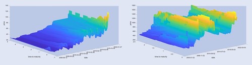
We use historical future data from 01/01/2006 till 01/01/2023 for both salmon⁵ and soybeans. This is illustrated in figure 1. For the plots we used a nearest neighbor interpolation for fixed date in the direction of the time-to-maturity. A dark blue color reflects low prices, while a bright yellow color reflects high prices relative to the individual commodity. On the left-hand side, we can see the evolution of the salmon future prices over time for different time-to-maturities and on the right-hand side for the soybean futures. Notably, the volatility of these prices seems to increase significantly at the end during the Covid pandemic. For salmon the prices seem to increase steadily over time with more rapid increase recently. If we estimate the spot prices from the smallest time-to-maturity in these pictures, we can also observe that the majority of the behavior of the future prices is determined by the spots, since they appear almost constant or with non-rapid fluctuations on the time-to-maturity axis for a fixed date.

Figure 1. Interpolated (nearest neighbor) market future surfaces for salmon (left) and soy (right) from 01/01/2006 till 01/01/2023. On the x-axis are dates identified by integers, on the y-axis the time-to-maturity and on the z-axis the corresponding price. Deep blue associates a low and yellow a high price.

3.2. Calibration to market data

At the start of this section, we would like to remind the reader about two well-known techniques for the calibration of multi-factor commodity pricing models with hidden state variables to historical futures price data. Since our commodity models are uncoupled, we will omit once again the dependence on the individual commodities throughout this entire section. The first was introduced by Cortazar and Schwartz (2003) as a nested least square regression, the second one is using a Kalman filter (cf. Schwartz 1997).

The goal is to find both the model parameters $\mathrm{\Pi }:=[{\sigma }_1,{\sigma }_2,\kappa ,\alpha ,\lambda ,\rho ],$ and the unobservable spots and convenience yields for each date $S\ge 0$, $\delta \in \mathbb{R}$.

For the calibration procedure, we will restrict ourselves to a subset of the main dataset. In fact, we only consider the slice from 01/01/2018 to 01/01/2022, taking only the most recent price developments into account making a regime-switching model unnecessary.

We will denote in this section the number of days, where market future prices are available by $K\in \mathbb{N}$ and for each date the number of available maturities by $P_i\in \mathbb{N}$. The market future prices at date $i=1,\dots ,K$ with time-to-maturity $\mathrm{\Delta }{T}_j$, $j=1,\dots ,P_i$ will be denoted by $F_{\mathrm{ij}}^{\mathrm{Market}}$ and the model future prices depending on the parameters Π by $F^{\mathrm{\Pi }}$.

3.2.1. Cortazar and Schwartz (2003)

We would like to minimize the following objective: $\underset{\mathrm{\Pi }}{min}\sum _{i=1}^K\sum _{j=1}^{P_i}{(\log F^{\mathrm{\Pi }}(S_{t_i},{\delta }_{t_i},T_j-t_i)-\log F_{\mathrm{ij}}^{\mathrm{Market}})}^2$ subject to $\begin{array}{rl}& (S_{t_i},{\delta }_{t_i})\in {\mathrm{argmin}}_{S,\delta }\sum _{j=1}^{P_i}(\log F^{\mathrm{\Pi }}(S,\delta ,T_j-t_i)\\ & {-\log F_{\mathrm{ij}}^{\mathrm{Market}})}^2\mathrm{for}\mathrm{all}i=1,\dots ,N.\end{array}$ We need the constraint since the spot price and convenience yield are not observable. The optimization for the state variables $S_{t_i},{\delta }_{t_i}$ can be solved efficiently by a linear least-square regression and for minimizing the objective we use matlab's fmincon with the interior-point method. This is a simplified version of the algorithm presented in Cortazar and Schwartz (2003). It is only used to stress that the model future prices are mostly determined by the unobservable state variables and can provide an equally good fit to the market future prices for very different parameters Π.

3.2.2. Kalman filtering

Following Schwartz (1997, pp. 10 ff.), the idea is to first discretize the log-spot price $s_t:=\log \left(S_t\right)$ and convenience yield under the historical measure $\mathbb{P}$, e.g. by using an Euler–Maruyama scheme. They are both normally distributed. Thus, for a homogeneous time grid $(t_i{)}_{i=1,\dots ,K}$ with step-size $\mathrm{\Delta t}$, we have $\begin{array}{rl}{s}_{t_{i+1}}& =s_{t_i}+(\mu -{\delta }_{t_i}-\frac{1}{2}{\sigma }_1^2)\mathrm{\Delta t}+{\sigma }_1\mathrm{\Delta }{W}_{t_i}^1,\\ {\delta }_{t_{i+1}}& ={\delta }_{t_i}+(\kappa (\alpha -{\delta }_{t_i})-\lambda )\mathrm{\Delta t}+{\sigma }_2\mathrm{\Delta }{W}_{t_i}^2.\end{array}$ Letting $X_{t_i}:=[s_{t_i},{\delta }_{t_i}{]}^{\mathrm{\top }}$ we have the transition equation $\begin{array}{rl}{X}_{t_{i+1}}& =c+T\cdot X_{t_i}+{\eta }_i,\\ c& :=\left[\begin{array}{c}r-\frac{1}{2}{\sigma }_1^2\\ \mathrm{\kappa \alpha }\end{array}\right]\mathrm{\Delta t},T:=\left[\begin{array}{cc}1& -\mathrm{\Delta t}\\ 0& 1-\kappa \mathrm{\Delta t}\end{array}\right],\\ E& :=\left[\begin{array}{cc}{\sigma }_1^2& \rho {\sigma }_1{\sigma }_2\\ \rho {\sigma }_1{\sigma }_2& {\sigma }_2^2\end{array}\right]\mathrm{\Delta t}\end{array}$ in a so-called state–space formulation. Here ${\eta }_i\sim \mathcal{N}(0,E)$ is serially uncorrelated. Since the spot prices are non-observable, we need to measure them. For this we use the log-future prices with different time-to-maturities $\mathrm{\Delta }{T}_j$ to derive the measurement equation $\begin{array}{rl}{Y}_{t_i}& ={\left[d\right(\mathrm{\Delta }{T}_j\left)\right]}_{j=1,\dots ,P}+{\left[Z\right(\mathrm{\Delta }{T}_j\left)\right]}_{j=1,\dots ,P}\cdot X_{t_i}+{ϵ}_i,\\ j& =1,\dots ,P,P\in \mathbb{N},\\ d\left(\mathrm{\Delta T}\right)& :=A\left(\mathrm{\Delta T}\right),Z\left(\mathrm{\Delta T}\right):=\left[\begin{array}{cc}1& \frac{-(1-e^{-\kappa \mathrm{\Delta t}}}{\kappa })\end{array}\right],\\ D& :=\mathrm{diag}(d_1^2,\dots ,d_P^2),\end{array}$ where ${ϵ}_i\sim \mathcal{N}(0,D)$ is serially uncorrelated and independent of η. Note that ϵ has to be added as measurement noise to make the model compatible for Kalman filtering. The choice of the covariance matrix has a significant impact on the estimation. We chose in our implementation a diagonal covariance matrix D. This choice seems to be the standard for commodity models and has already been used by Schwartz (1997).

Using different panels, i.e. a collection of different time-to-maturities $\mathrm{\Delta }{T}_j$, can yield significantly different parameters. The panels are assumed to be fixed throughout the entire filtering, which is a disadvantage compared to Cortazar and Schwartz (2003), since it can use the entire data set without any interpolation or averaging. To compare the Kalman filter to the method by Cortazar and Schwartz (2003), we use a daily time step for the Kalman filter as well.

The parameters can now be estimated by maximizing the likelihood of $Y_{t_i}$ equaling the market log-future prices and meanwhile estimating the unobservable spot prices and convenience yields by the Kalman filter. For more details, we refer to the code and the monographs Harvey (1989, pp. 100 ff. Chapter 3) and Bishop (2006, pp. 635 ff. Chapter 13.3). We use matlab's fmincon with the interior-point method to minimize the negative log-likelihood.

3.2.3. Model uncertainty

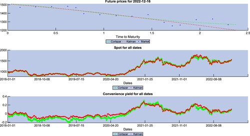
In figure 2, we compare some calibration results using the soybean data from 01/01/2018 till 01/01/2022 using both a Kalman filter and Cortazar and Schwartz (2003). We found the following parameters: $\begin{array}{rl}{\mathrm{\Pi }}^{\mathrm{Kalman}}& =[0.2044,0.1275,0.1541,0.3355,\\ & 0.0101,0.9065],\\ {\mathrm{\Pi }}^{\mathrm{CS}}& =[2.1975,0.4594,0.4381,\\ & 2.2825,1.3120,0.4893].\end{array}$ The red color will show all the results using ${\mathrm{\Pi }}^{\mathrm{Kalman}}$ and the green color for ${\mathrm{\Pi }}^{\mathrm{CS}}$. In the upper third of the figure, we compare the model future prices to the market future prices for different time-to-maturities on the 16/12/2022, which was randomly chosen. We can see that both models seem to regress the market prices (blue crosses) appropriately and they are very close to each other. In the middle part of the figure, we compare the inferred spot prices $S_0$ for each date from 01/01/2018 till 01/01/2022. We can also see that both calibration methods seem to find very similar spot prices. A little bit more variation can be seen in the inferred convenience yields in the lower part of the figure, but still very similar. We would like to stress at this point that the model seems to produce very similar results with extremely different parameters. If one only needs to find the unobservable spot prices or fit the model to futures prices, then both methods perform equally well, but if one needs the underlying model for more complex decision making, this raises a major concern, as in our case. In fact, for the real option discussed in this paper, the model parameters will have a significant impact on the harvesting decision and the valuation of the business. We will address this problem further in future research.

Figure 2. Close spot and future prices for different model parameters.

We believe that the Kalman filter underestimates the real volatility, while the method by Cortazar and Schwartz (2003) overestimates it. Since there seems to be a lot of uncertainty in finding appropriate parameters for our commodity models, we will use the artificial parameters shown in tables 2 and 3 for our further investigation. These are based on the calibration results, and chosen such that we can discuss the question of whether stochastic feeding costs should be considered in aquaculture investment or whether the effect is negligible. The mean relative price changes of the commodity models using the different parameters are illustrated in figure 3. The left subfigure shows the salmon prices. The red line corresponds to the scenario down, down, the green line to down, up, and the blue line to up, up. Similarly for the soy spot prices in the right subfigure. The red line corresponds to the scenario low volatility, the green line corresponds to medium volatility, and the blue line corresponds to high volatility.

Figure 3. Mean relative changes of salmon (left) and soy (right) prices for the different scenarios in tables 2 and 3.

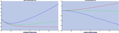
Table 3. Parameters for different scenarios of soybean models.

Scenario	${\sigma }_1^2$	${\sigma }_2^2$	${\kappa }^2$	${\alpha }^2$	${\lambda }^2$	${\rho }^2$	${\delta }_0^2$	${\hat{S}}_0^2$
Low volatility	0.5	0.4	1.2	0.06	0.14	0.44	0	1500
Medium volatility	1	0.4	1.2	0.06	0.14	0.44	0	1500
High volatility	2	0.4	1.2	0.06	0.14	0.44	0	1500

We performed many tests and found that the most sensitive parameter for estimating the benefit of using stochastic feeding costs is ${\sigma }_1^2$ for a given salmon scenario. Moreover, the closer the feeding costs are to the salmon revenue, the more the feeding costs matter, which explains our choices for selecting the salmon scenarios such that we have a mean decrease, mean stable, and mean increase scenario in prices. This could be achieved by only adjusting the risk-premium parameter ${\lambda }^1$, since it changes the drift of the convenience yield and thus the drift of the spot price.

We have made the code publicly available and encourage the reader to try other parameter configurations.

3.3. Comparison of exercise decisions

To compare the optimal exercise decisions in the different feeding cost scenarios, we will employ a pathwise comparison of the stopping times. Let $(\mathrm{\Omega },\mathcal{F},{\mathcal{F}}_t,\mathbb{P})$ be a filtered probability space satisfying the usual conditions, where ${\mathcal{F}}_t:=\sigma \left(X_t\right)$ is generated by a stochastic process, and ${\mathcal{F}}_t^i\subseteq {\mathcal{F}}_t$, i = 1, 2, be two sub-σ-filtrations. Moreover, let ${\tau }^1$ be an (${\mathcal{F}}_t^1$)- stopping time and ${\tau }^2$ an (${\mathcal{F}}_t^2$)- stopping time. Now, let us fix a path $\left(X_t\right(\omega ){)}_{t\ge 0}$, then conditioned on this path the two stopping times ${\tau }^1\left(\omega \right)\in [0,T]$ and ${\tau }^2\left(\omega \right)\in [0,T]$ can be compared as real numbers.

Additionally, still conditioned on $\left(X_t\right(\omega ){)}_{t\ge 0}$, we may compare the stopped values of a stochastic process $Y_t$, i.e. $Y_{{\tau }^1\left(\omega \right)}$ and $Y_{{\tau }^2\left(\omega \right)}$.

3.4. Results

In this section, we will assume stochastic feeding costs and demonstrate the differences and improvements when the optimal stopping rules obtained from accounting for stochastic feeding costs are employed as compared to the case where deterministic feeding costs are assumed. We compare all the different scenarios using all the combinations of the parameters given in tables 2 and 3. For the pathwise comparison of the stopping times, we used $M=10000$ simulations in the LSMC, which takes roughly 1 second (roughly 0.6 seconds to generate the stochastic processes and 0.1 for the actual LSMC algorithm) on the CPU in the case of stochastic feeding costs. We repeat these calculations $m=10000$ times to compute the $95\mathrm{\%}$ confidence intervals of our results. We used standard polynomials (monomials) up to degree 2 as a regression basis.

In table 4, we show a metric for the relative improvement of using stochastic feeding costs compared to deterministic feeding costs. For this we use the pathwise comparison denoted by ${\mathrm{RI}}^{\tau }:=\frac{V_0^{\tau ,\mathrm{stoch}}}{V_0^{\tau ,\mathrm{determ}}}$. The value is the mean of the $m=10000$ trials as aforementioned and in brackets are the $95\mathrm{\%}$ confidence intervals.

Table 4. Relative improvements using stochastic feeding costs. Mean with confidence intervals using $m=10000$ trials each with $M=10000$ simulations for LSMC.

	Salmon
Soy	Down, down	Down, up	Up, up
Low vol	${\mathrm{RI}}^{\tau }=1.0045$	${\mathrm{RI}}^{\tau }=1.0027$	${\mathrm{RI}}^{\tau }=1.0004$
	$(1.0040,1.0051)$	$(1.0020,1.0034)$	$(0,9999,1.0010)$
Medium vol	${\mathrm{RI}}^{\tau }=1.0301$	${\mathrm{RI}}^{\tau }=1.01940$	${\mathrm{RI}}^{\tau }=1.0052$
	$(1.0296,1.0307)$	$(1.0187,1.0200)$	$(1.0046,1.0058)$
High vol	${\mathrm{RI}}^{\tau }=1.1203$	${\mathrm{RI}}^{\tau }=1.0926$	${\mathrm{RI}}^{\tau }=1.0478$
	$(1.1195,1.1211)$	$(1.0918,1.0934)$	$(1.0472,1.0485)$

As expected, we note in the case of low vol (first row of table 4) that the benefit of using a stopping rule accounting for the stochastic nature of the feed costs is only slightly better than its deterministic counterpart. In this case, deterministic feeding costs seem to be a good approximation. The benefit of using stochastic feeding costs, however, increases up to $11.6\mathrm{\%}$ the higher the volatility, for the scenario of declining salmon prices.

In table 5, we present the corresponding values of the fish farm (4(4) $\begin{array}{rl}{V}_0^z\left(x\right)& :={\mathbb{E}}^{\mathbb{Q}}[\exp (-r{\tau }^z)\left(S_{{\tau }^z}^1\mathrm{B}\right({\tau }^z)-\mathrm{CH}({\tau }^z\left)\right)\\ & -{\mathrm{CF}}^{\mathrm{stoch}}\left({\tau }^z\right)|X_0^{\mathrm{stoch}}=x]\end{array}$(4) ) using the different stopping rules for all of the scenario combinations. We only present the mean of the $m=10000$ trials in this table to make it more readable and refer the reader to the code⁶ for the quite narrow confidence intervals and other statistics. Furthermore, we stress how much these values change in relation to changes in the risk-premium ${\lambda }^1$, showing that the decision making in the real option is very sensitive to the model parameters.

Table 5. Value of (4(4) $\begin{array}{rl}{V}_0^z\left(x\right)& :={\mathbb{E}}^{\mathbb{Q}}[\exp (-r{\tau }^z)\left(S_{{\tau }^z}^1\mathrm{B}\right({\tau }^z)-\mathrm{CH}({\tau }^z\left)\right)\\ & -{\mathrm{CF}}^{\mathrm{stoch}}\left({\tau }^z\right)|X_0^{\mathrm{stoch}}=x]\end{array}$(4) ) using stochastic feeding costs with different stopping rules.

	Salmon
Soy	Down, down	Down, up	Up, up
Low vol	$V_0^{\tau ,\mathrm{determ}}=1922265$	$V_0^{\tau ,\mathrm{determ}}=2397588$	$V_0^{\tau ,\mathrm{determ}}=3897333$
	$V_0^{\tau ,\mathrm{stoch}}=1930654$	$V_0^{\tau ,\mathrm{stoch}}=2403022$	$V_0^{\tau ,\mathrm{stoch}}=3898161$
Medium vol	$V_0^{\tau ,\mathrm{determ}}=1951032$	$V_0^{\tau ,\mathrm{determ}}=2429512$	$V_0^{\tau ,\mathrm{determ}}=3933336$
	$V_0^{\tau ,\mathrm{stoch}}=2009449$	$V_0^{\tau ,\mathrm{stoch}}=2475496$	$V_0^{\tau ,\mathrm{stoch}}=3952845$
High vol	$V_0^{\tau ,\mathrm{determ}}=2004857$	$V_0^{\tau ,\mathrm{determ}}=2488747$	$V_0^{\tau ,\mathrm{determ}}=3998265$
	$V_0^{\tau ,\mathrm{stoch}}=2244406$	$V_0^{\tau ,\mathrm{stoch}}=2717344$	$V_0^{\tau ,\mathrm{stoch}}=4187842$

Let us focus on the first column in table 5, the down, down scenario. The values $V_0^{\tau ,\mathrm{determ}}$ are close to each other regardless of the volatility scenario for the feeding costs. On the other hand, the values $V_0^{\tau ,\mathrm{stoch}}$ differ significantly and increase with higher volatility. This means if the model is misspecified with e.g. too low volatility, then the deterministic stopping rules will produce less revenue than the stochastic stopping rules, which can benefit from the higher volatility.

If the initial feeding costs would have been $50\mathrm{\%}$ of the production costs, then e.g. in the case down, up with medium vol the benefit of using stochastic feeding costs would increase to roughly $8\mathrm{\%}$. This is similar for all the other cases as well and highlights the importance of determining the correct relationship of salmon revenue and feeding costs. For feeding costs between $25\mathrm{\%}$ and $50\mathrm{\%}$ of the production costs the benefit will lie in between $1.5\mathrm{\%}$ and $8\mathrm{\%}$. Thus the benefits presented in table 4 can be understood as a lower bound.

4. Conclusion

In this article, we focused on the question of whether accounting for stochastic feeding costs can significantly improve aquaculture decision making and increase the financial value of an aquaculture business as compared to the case when deterministic feeding costs are assumed. We found a partial answer: if the volatility of the feed price is high enough, then it is beneficial to use stochastic feeding costs, otherwise deterministic feeding costs can lead to an almost equal performance. In none of the cases, however, does the inclusion of stochastic feeding costs lead to impaired performance, and as the computational effort only marginally increases when using our proposed methodology, we highly recommend to adopt relevant models to account for feeding cost risk.

We found that there is a lot of model uncertainty, highlighted by the significantly different parameters obtained from Kalman filtering and the technique by Cortazar and Schwartz (2003). Since this has a major impact on the real option, both value and exercise, it needs to be addressed in future work. To this end, we would like to add a control to the objective (3(3) $\begin{array}{rl}{W}_0^{\mathrm{determ}}\left(x\right)& :=\underset{{\tau }^{\mathrm{determ}}}{sup}{\mathbb{E}}^{\mathbb{Q}}[\exp (-\mathrm{r\tau })\left(S_{\tau }^1\mathrm{B}\right(\tau )-\mathrm{CH}(\tau \left)\right)\\ & -{\mathrm{CF}}^{\mathrm{determ}}\left(\tau \right)|X_0^{\mathrm{determ}}=x].\end{array}$(3) ) in terms of a model-free decision rule, based on so-called myopic look ahead and k-step ahead rules (cf. Ross 1971). It might be possible to add such a control also to the Kalman filter allowing for more robust parameter estimations.

In the line of feeding costs, we have seen that the relative difference of the salmon prices to the feeding costs is important. If salmon prices are much higher/lower than feeding costs and tend to increase/decrease a lot, then the stochastic nature of the feeding costs may be negligible/dominating. To investigate this further, one could also study a more realistic case, in which storage for the feed is available, as well as optimal pairs of buying time and buying quantity combined with an adjustable feeding rate per day. Another opportunity for future research is to further investigate the correlation between salmon price and salmon feed and how this should be implemented and estimated in classical multi-factor commodity models. An application of reinforcement learning comes to mind to tackle this problem.

Moreover, we are interested in a case where the intercorrelations of the commodities may be stochastic as well. As this leads to a full correlation matrix, it can be modeled with a stochastic process taking values in an appropriate Lie-group like in Muniz et al. (2021). For this the techniques developed in Muniz et al. (2022) and Kamm et al. (2021) may be very helpful.

In Misund (2022, pp. 40–45), it is argued that biological costs due to, e.g. salmon lice treatments are of equal size to the feeding costs. Thus, in future studies, one should address a similar question for stochastic mortality or at an even deeper level of detail, look at how host–parasite models and costs for salmon lice treatments can be implemented with the classical salmon farm model.

Open Scholarship

This article has earned the Center for Open Science badges for Open Data and Open Materials through Open Practices Disclosure. The data and materials are openly accessible at https://github.com/kevinkamm/AquacultureStochasticFeeding.

Code availability

The Matlab/Python code and data sets to produce the numerical experiments are available at https://github.com/kevinkamm/AquacultureStochasticFeedinghttps://github.com/kevinkamm/AquacultureStochasticFeeding.

Acknowledgments

We would like to thank the anonymous reviewers for their comments and insights, which significantly improved this manuscript.

Disclosure statement

No potential conflict of interest was reported by the author(s).

Notes

1 With implicitly coupled we mean that the coupling mechanism is through possible correlation rather than an explicit coupling of the corresponding SDEs in the way that the soybean spot price occurs in the dynamics of the salmon spot price and vice versa. Allowing for implicit coupling is quite common in multi-commodity models, see, for example Ellefsen and Sclavounos (2009). An explicit coupling, however, would likely cause unprecedented challenges in computing futures prices and beyond this in the calibration of the model.

2 The stopping problem by itself could even be solved under the assumption of an explicit coupling, the LSMC algorithm does not present any major obstacles here. However, a good empirical calibration to future prices allowing for explicit coupling would be very hard to achieve, if not impossible.

3 We assume that the interest rate is deterministic and constant. Therefore, forward and future prices are the same, cf. Björk (2009, p. 456 Proposition 29.6).

4 The time derivative of the growth is denoted by ${\mathrm{\partial }}_t\mathrm{w}$ and given by $\left({\mathrm{\partial }}_t\mathrm{w}\right)\left(t\right)=3{\mathrm{w}}_{\mathrm{\infty }}(a-b{e}^{-\mathrm{ct}}{)}^{2}bc{e}^{-\mathrm{ct}}$. The term $\left({\mathrm{\partial }}_t\mathrm{w}\right)\left(s\right)$ captures the weight increase of one fish in kg, $\left({\mathrm{\partial }}_t\mathrm{w}\right)\left(s\right)\mathrm{c}$ the amount of feed in kg that is required for this growth, $\mathrm{n}\left(s\right)\left({\mathrm{\partial }}_t\mathrm{w}\right)\left(s\right)\mathrm{c}$ the total feed and finally ${\mathrm{F}}_s\mathrm{n}\left(s\right)\left({\mathrm{\partial }}_t\mathrm{w}\right)\left(s\right)\mathrm{c}$ the total cost.

5 The historical salmon future prices are publicly available onhttps://fishpool.eu/forward-price-history/ (last accessed 04/07/2023 12:45 CEST).

6 See https://github.com/kevinkamm/AquacultureStochasticFeeding/tree/main/Python/Statistics.

Appendix. The impact of intercorrelations

In this section, we will discuss the impact of intercorrelations of the two commodities. We will assume that all correlations are constant and deterministic. Since the spot prices and convenience yields of both commodities are unobservable, we discuss several different ways to infer the correlation from the future data using similar techniques as for the calibration.

We only have one realization of the time series and to eliminate effects from common drifts of the commodities such as inflation, we will use the first difference technique to extract all of our correlations. Moreover, it is implied that the distribution, from which we suspect the unobserved state variables to come from, is stationary. This allows us to consider for the computation of the correlation the time series as a vector of realizations from the same distribution and we can compute statistics on this. To be more precise, let $Z_{t_i}^j$, $i=1,\dots ,n$, j = 1, 2, be two time series, we compute the correlations at zero lag on the time series ${\hat{Z}}_{t_i}^j:=Z_{t_{i+1}}^j-Z_{t_i}^j$ and define $\begin{array}{rl}{\rho }_{12}& =\frac{\mathrm{Cov}({\hat{Z}}^1,{\hat{Z}}^2)}{\mathrm{Std}\left({\hat{Z}}^1\right)\mathrm{Std}\left({\hat{Z}}^2\right)},\\ \mathrm{Mean}\left({\hat{Z}}^j\right)& =\frac{1}{n}\sum _{i=1}^n{\hat{Z}}_{t_i}^j,\mathrm{Std}\left({\hat{Z}}^j\right)\\ & =\sqrt{\frac{1}{n}\sum _{i=1}^n{({\hat{Z}}_{t_i}^j-\mathrm{Mean}\left({\hat{Z}}^j\right))}^2}\\ \mathrm{Cov}({\hat{Z}}^1,{\hat{Z}}^2)& =\frac{1}{n}\sum _{i=1}^n({\hat{Z}}_{t_i}^1-\mathrm{Mean}\left({\hat{Z}}^1\right))({\hat{Z}}_{t_i}^2-\mathrm{Mean}\left({\hat{Z}}^2\right)).\end{array}$ In our experiments we have n = 754 coming from roughly 250 business days per year over the time span of 3 years. Using matlab's 2023a's corrcoeff under standard assumptions this implies that only correlations outside of the interval $[-0.07,0.07]$ can be considered as statistically significant. This result is based on the classical assumption that the standard errors follow a student's t-distribution.

A.1. From filtered spots

Both the Kalman filter and the method by Cortazar and Schwartz (2003) give an estimate of the log-spot prices and the convenience yield. We use these time series to conduct our correlation study in this section. Define $Z_{t_i}:=(Z_{t_i}^1,Z_{t_i}^2,Z_{t_i}^3,Z_{t_i}^4):=({\hat{X}}_{t_i}^1,{\hat{\delta }}_{t_i}^1,{\hat{X}}_{t_i}^2,{\hat{\delta }}_{t_i}^2)$, then we have for example that the correlation of ${\hat{Z}}_{t_i}^1$ and ${\hat{Z}}_{t_i}^3$ represents the correlation between the log-spot prices of salmon and soybean.

In table A1, we show the intracorrelations ${\rho }_{12},{\rho }_{34}$ together with the intercorrelations inferred from the filtered time series. The first column refers to the panel used in the computation of the Kalman filter, so future contracts with maturities of x months. We used the same panel for both commodities. We can see that most of the correlations are similar among different panels, except for the intra-correlation of soybean log price and convenience yield. All the intercorrelations are less than $\left|\rho \right|\le 0.065$, which we interpret as insignificant. Similarly, using the inferred log-spot prices and convenience yields using the method by Cortazar and Schwartz (2003) yields the following correlations: ${\rho }_{12}=0.9572$, ${\rho }_{13}=0.0507$, ${\rho }_{14}=0.0385$, ${\rho }_{23}=0.0641$, ${\rho }_{24}=0.0489$ and ${\rho }_{34}=0.9446$. Again the intercorrelations appear to be insignificant.

Table A1. Correlation matrix inferred from filtered log-spot prices and convenience yield using two separate Kalman filters for salmon and soybean.

Panel	${\rho }_{12}$	${\rho }_{13}$	${\rho }_{14}$	${\rho }_{23}$	${\rho }_{24}$	${\rho }_{34}$
$[1,2,3,4,5,6]$	0.9560	0.0225	−0.0107	0.0130	−0.0244	0.4957
$[1,2,6,7,11,12]$	0.9334	0.0133	0.0058	−0.0151	−0.0261	0.7849
$[6,7,11,12,15,16]$	0.9833	−0.0596	−0.0382	−0.0679	−0.0436	0.9232

A.2. Joint Kalman filter

Let us briefly derive the state–space model for the joint Kalman filter under the historical measure $\mathbb{P}$ for both salmon and soybeans. The assumption is that all the Brownian motions involved are correlated. Then we can proceed exactly like Schwartz (1997, pp. 10 ff.). We denote with $X_t^i:=\log \left(S_t\right)$ the log-spot price, whose dynamics is given by $\mathrm{d}{X}_t^i=({\mu }^i-\frac{1}{2}({\sigma }_1^i{)}^2-{\delta }_t^i)\mathrm{d}t+{\sigma }_1^i\mathrm{d}{W}_t^{i,1}.$ We discretize both $X^i$ and ${\delta }^i$ by the Euler–Maruyama scheme on a homogeneous time grid ${\mathcal{T}}^n:=\left\{\right(t_k{)}_{k=1,\dots ,n}:t_k=(k-1)\mathrm{\Delta t},\mathrm{\Delta t}=\frac{T}{(n-1)}\}$, i.e. for $\mathrm{\Delta }{W}_{t_k}:=W_{t_{k+1}}-W_{k_i}$ $\begin{array}{rl}{X}_{t_{k+1}}^i& =X_{t_k}^i+({\mu }^i-\frac{1}{2}({\sigma }_1^i{)}^2-{\delta }_{t_k}^i)\mathrm{\Delta t}+{\sigma }_1^i\mathrm{\Delta }{W}_{t_k}^{i,1},\\ {\delta }_{t_{k+1}}^i& ={\delta }_{t_k}^i+{\kappa }^i({\alpha }^i-{\delta }_{t_k}^i)\mathrm{\Delta t}+{\sigma }_2^i\mathrm{\Delta }{W}_{t_k}^{i,2}.\end{array}$ Now, we want to find matrices $c_t,Q_t,{\mathrm{\Sigma }}_t$, such that the transition equation is given by $\begin{array}{rl}{[X_{t_k}^1,{\delta }_{t_k}^1,X_{t_k}^2,{\delta }_{t_k}^2]}^{\mathrm{\top }}& =c_{t_k}+Q_{t_k}{[X_{t_{k-1}}^1,{\delta }_{t_{k-1}}^1,X_{t_{k-1}}^2,{\delta }_{t_{k-1}}^2]}^{\mathrm{\top }}+{\eta }_{t_k},\\ & {\eta }_{t_k}\sim \mathcal{N}(0,{\mathrm{\Sigma }}_{t_k}),\end{array}$ where ${\eta }_t$ are serially uncorrelated and we want to find matrices $d_t,Z_t,H_t$, such that the measurement equation ($Y_t$ takes the role of the log-future prices of both commodities) is given by $\begin{array}{rl}& Y_{t_k}(\mathrm{\Delta }{T}^1,\mathrm{\Delta }{T}^2)\\ & =d_{t_k}(\mathrm{\Delta }{T}^1,\mathrm{\Delta }{T}^2)+Z_{t_k}(\mathrm{\Delta }{T}^1,\mathrm{\Delta }{T}^2){[X_{t_k}^1,{\delta }_{t_k}^1,X_{t_k}^2,{\delta }_{t_k}^2]}^{\mathrm{\top }}\\ & +{ϵ}_{t_k},{ϵ}_t\sim \mathcal{N}(0,H_t),\end{array}$ where ${ϵ}_t$ are serially uncorrelated and $\mathrm{\Delta }{T}^i$ refers to the time-to-maturity for the future contracts of the commodities i = 1, 2.

The coefficients for the transition equation are given by $\begin{array}{rl}{c}_t& \equiv {[{\mu }^1-\frac{1}{2}({\sigma }_1^1{)}^2,{\kappa }^1{\alpha }^1,{\mu }^2-\frac{1}{2}({\sigma }_1^2{)}^2,{\kappa }^2{\alpha }^2,]}^{\mathrm{\top }},\\ Q_t& \equiv \left[\begin{array}{cccc}1& -\mathrm{\Delta t}& 0& 0\\ 0& 1-{\kappa }^1\mathrm{\Delta t}& 0& 0\\ 0& 0& 1& -\mathrm{\Delta t}\\ 0& 0& 0& 1-{\kappa }^2\mathrm{\Delta t}\end{array}\right],\\ {\mathrm{\Sigma }}_t^2& \equiv \left[\begin{array}{cccc}({\sigma }_1^1{)}^2& {\sigma }_1^1{\sigma }_2^1{\rho }_{12}& {\sigma }_1^1{\sigma }_1^2{\rho }_{13}& {\sigma }_1^1{\sigma }_2^2{\rho }_{14}\\ {\sigma }_2^1{\sigma }_1^1{\rho }_{12}& ({\sigma }_2^1{)}^2& {\sigma }_2^1{\sigma }_1^2{\rho }_{23}& {\sigma }_2^1{\sigma }_2^2{\rho }_{24}\\ {\sigma }_1^2{\sigma }_1^1{\rho }_{13}& {\sigma }_1^2{\sigma }_2^1{\rho }_{23}& ({\sigma }_1^2{)}^2& {\sigma }_1^2{\sigma }_2^2{\rho }_{34}\\ {\sigma }_2^2{\sigma }_1^1{\rho }_{14}& {\sigma }_2^2{\sigma }_2^1{\rho }_{24}& {\sigma }_2^2{\sigma }_1^2{\rho }_{34}& ({\sigma }_2^2{)}^2\end{array}\right]\mathrm{\Delta t}.\end{array}$ Let $F^i\left(\mathrm{\Delta }{T}^i\right)$ denote the future prices (1(1) $\begin{array}{rl}F(S,\delta ,\mathrm{\Delta T})& =\mathrm{Sexp}(-\delta \frac{1-e^{-\kappa \mathrm{\Delta T}}}{\kappa }+A(\mathrm{\Delta T}\left)\right),\\ A\left(\mathrm{\Delta T}\right)& =(r-\hat{\alpha }+\frac{1}{2}\frac{{\sigma }_2^2}{{\kappa }^2}-\frac{{\sigma }_1{\sigma }_2}{\kappa })\mathrm{\Delta T}\\ & +\frac{1}{4}{\sigma }_2^2\frac{1-e^{-2\kappa \mathrm{\Delta T}}}{{\kappa }^3}\\ & +(\hat{\alpha }\kappa +{\sigma }_1{\sigma }_2\rho -\frac{{\sigma }_2^2}{\kappa })\frac{1-e^{-\kappa \mathrm{\Delta T}}}{{\kappa }^2},\end{array}$(1) ). The coefficients for the measurement equation are given by $\begin{array}{rl}{Y}_{t_k}(\mathrm{\Delta }{T}^1,\mathrm{\Delta }{T}^2)& =[\log F^1(S_{t_k}^1,{\delta }_{t_k}^1,\mathrm{\Delta }{T}^1),\log F^1(S_{t_k}^1,{\delta }_{t_k}^1,\mathrm{\Delta }{T}^1){]}^{\mathrm{\top }},\\ d_{t_k}(\mathrm{\Delta }{T}^1,\mathrm{\Delta }{T}^2)& =\left[A^1\right(\mathrm{\Delta }{T}^1),A^2(\mathrm{\Delta }{T}^2){]}^{\mathrm{\top }},\\ Z_t(\mathrm{\Delta }{T}^1,\mathrm{\Delta }{T}^2)& =\left[\begin{array}{cccc}1& -\frac{1-e^{-{\kappa }^1\mathrm{\Delta }{T}^1}}{{\kappa }^1}& 0& 0\\ 0& 0& 1& -\frac{1-e^{-{\kappa }^2\mathrm{\Delta }{T}^2}}{{\kappa }^2}\end{array}\right],\\ H_t& \equiv \mathrm{diag}(h_1,h_2),\end{array}$ with the obvious changes if there are multiple maturities in the different panels of the two commodities.

In table A2, we show the parameters found by the joint Kalman filter and in table A3 we show similar to table A1 the correlations inferred from the filtered log-spot prices and convenience yield. Again, we present the correlations for different panels used in the Kalman filter, we used the same panels for both commodities. In all cases, the values of tables A2 and A3 are very close, which also serves to validate our choice of using the first difference technique for the filtered time series. In these tests, the values of the correlations except for ${\rho }_{12}$ differ among the different panels, which raises the question of parameter uncertainty and the suitability of the Kalman filter for this problem again.

Table A2. Correlation matrix deduced by a joint Kalman filter for salmon and soybean.

Panel	${\rho }_{12}$	${\rho }_{13}$	${\rho }_{14}$	${\rho }_{23}$	${\rho }_{24}$	${\rho }_{34}$
$[1,2,3,4,5,6]$	0.944	0.011004	0.13451	0.052189	0.1236	0.19658
$[1,2,6,7,11,12]$	0.93374	0.030779	0.11054	0.058464	0.09726	0.52233
$[6,7,11,12,15,16]$	0.99687	−0.16528	−0.10078	−0.16908	−0.10595	0.87066

Table A3. Correlation matrix inferred from filtered log-spot prices and convenience yield using a joint Kalman filter for salmon and soybean.

Panel	${\rho }_{12}$	${\rho }_{13}$	${\rho }_{14}$	${\rho }_{23}$	${\rho }_{24}$	${\rho }_{34}$
$[1,2,3,4,5,6]$	0.9501	0.0637	0.1328	0.0826	0.1310	0.1259
$[1,2,6,7,11,12]$	0.9500	0.0612	0.0910	0.0727	0.0751	0.5784
$[6,7,11,12,15,16]$	0.9963	−0.1886	−0.1406	−0.1932	−0.1467	0.8852

Moreover, in all cases, we have for the intercorrelations $\left|\rho \right|\le 0.2$. This is higher than in section A.1 but still not a particular high correlation either, but now we have some statistically significant correlations. We show in the third part of the appendix though, that the impact of correlations of this magnitude is very minor while performance improvement through the inclusion of stochastic feed-costs (whether correlated or not) is still being guaranteed.

A.3. Case study

In this small section, we investigate the impact of the intercorrelations on the gain due to using a stochastic feeding model and the farm value using the stopping rule based on stochastic feeding costs.

Let ${\rho }^1$ and ${\rho }^2$ denote the correlations from tables 2 and 3, respectively. We define our test correlation matrix as follows: $\rho :[-1,1]\to {\mathbb{R}}^{4,4},\rho \left(x\right):=\left[\begin{array}{cccc}1& {\rho }^1& x& x\\ {\rho }^1& 1& x& x\\ x& x& 1& {\rho }^2\\ x& x& {\rho }^2& 1\end{array}\right].$ Since the highest intercorrelation we saw in the previous sections was $\pm 0.2$ we perform two tests in all scenarios with all parameters as in tables 2 and 3 but now with the full correlation matrices $\rho \left(0.2\right)$ and $\rho (-0.2)$. We add in table A4 the relative improvements, defined in section 3.4, denoted by ${\mathrm{RI}}^{+}$ and ${\mathrm{RI}}^{-}$, respectively, to table 4. Each entry contains the mean of $m=10000$ runs with $M=10000$ simulations for the LSMC algorithm and the $95\mathrm{\%}$ confidence intervals.

Table A4. Relative improvements using stochastic feeding costs with full correlation matrix.

	Salmon
Soy	Down, down	Down, up	Up, up
Low vol	${\mathrm{RI}}^{\tau }=1.0045$	${\mathrm{RI}}^{\tau }=1.0027$	${\mathrm{RI}}^{\tau }=1.0004$
	$(1.0040,1.0050)$	$(1.0020,1.0034)$	$(0.9998,1.0010)$
	${\mathrm{RI}}^{+}=1.0049$	${\mathrm{RI}}^{+}=1.0023$	${\mathrm{RI}}^{+}=1.0004$
	$(1.0045,1.0053)$	$(1.0017,1.0029)$	$(0.9998,1.0010)$
	${\mathrm{RI}}^{-}=1.0045$	${\mathrm{RI}}^{-}=1.0018$	${\mathrm{RI}}^{-}=1.0004$
	$(1.0041,1.0049)$	$(1.0011,1.0019)$	$(0.9998,1.0010)$
Medium vol	${\mathrm{RI}}^{\tau }=1.0301$	${\mathrm{RI}}^{\tau }=1.0194$	${\mathrm{RI}}^{\tau }=1.0052$
	$(1.0306,1.0296)$	$(1.0188,1.0200)$	$(1.0046,1.0058)$
	${\mathrm{RI}}^{+}=1.0293$	${\mathrm{RI}}^{+}=1.0194$	${\mathrm{RI}}^{+}=1.0058$
	$(1.0289,1.0297)$	$(1.0189,1.0199$	$(1.0053,1.0063)$
	${\mathrm{RI}}^{-}=1.0299$	${\mathrm{RI}}^{-}=1.0179$	${\mathrm{RI}}^{-}=1.0043$
	$(1.0295,1.0303)$	$(1.0173,1.0185)$	$(1.0036,1.0050)$
High vol	${\mathrm{RI}}^{\tau }=1.1203$	${\mathrm{RI}}^{\tau }=1.0926$	${\mathrm{RI}}^{\tau }=1.0478$
	$(1.1195,1.1211)$	$(1.0934,1.0918)$	$(1.0472,1.0484)$
	${\mathrm{RI}}^{+}=1.1110$	${\mathrm{RI}}^{+}=1.0883$	${\mathrm{RI}}^{+}=1.0478$
	$(1.1104,1.1116)$	$(1.0876,1.0890)$	$(1.0471,1.0485)$
	${\mathrm{RI}}^{-}=1.1252$	${\mathrm{RI}}^{-}=1.0941$	${\mathrm{RI}}^{-}=1.0471$
	$(1.1245,1.1259)$	$(1.0933,1.0949)$	$(1.0464,1.0478)$

We can see that the intercorrelations had almost no impact on the relative improvements due to the stochastic stopping rule, except in the high-volatility scenario combined with the decreasing salmon price with a difference of roughly $1\mathrm{\%}$ between the case without intercorrelations and the positive intercorrelations.

In table A5, we present the impact of the positive and negative correlations scenario on the farm value $W_0^{\mathrm{stoch}}$. We can see in all cases, that negative intercorrelations will lessen the farm value and positive intercorrelations will increase the farm value. This is intuitive, as salmon prices contribute to revenue and soy bean prices to cost, so a positive correlation achieves some diversification affect in the profits while negative correlations have the opposite effect. However, the changes in the farm value are very small for all the cases.

Table A5. Farm values using stochastic feeding costs with full correlation matrix.

	Salmon
Soy	Down, down	Down, up	Up, up
Low vol	$\rho =0$: 1 930 654	$\rho =0$: 2 403 022	$\rho =0$: 3 898 161
	$\rho =-0.2$: 1 925 131	$\rho =-0.2$: 2 397 483	$\rho =-0.2$: 3 896 229
	$\rho =0.2$: 1 937 654	$\rho =0.2$: 2 407 189	$\rho =0.2$: 3 899 199
Medium vol	$\rho =0$: 2 009 449,	$\rho =0$: 2 475 496	$\rho =0$: 3 952 845
	$\rho =-0.2$: 1 996 878	$\rho =-0.2$: 2 464 371	$\rho =-0.2$: 3 946 433
	$\rho =0.2$: 2 022 187	$\rho =0.2$: 2 486 452	$\rho =0.2$: 3 958 609
High vol	$\rho =0$: 2 244 406	$\rho =0$: 2 717 344	$\rho =0$: 4 187 842
	$\rho =-0.2$: 2 233 547	$\rho =-0.2$: 2 708 055	$\rho =-0.2$: 4 181 273
	$\rho =0.2$: 2 255 045	$\rho =0.2$: 2 728 003	$\rho =0.2$: 4 196 131

Since the code is publicly available, we invite the reader to use different parameters to validate these tests.

References

- Becker, S., Cheridito, P., Jentzen, A. and Welti, T., Solving high-dimensional optimal stopping problems using deep learning. Eur. J. Appl. Math., 2021, 32(3), 470–514. doi:10.1017/s0956792521000073
- Bishop, C.M., Pattern Recognition and Machine Learning (Information Science and Statistics), 2006 (Springer-Verlag: Berlin, Heidelberg).
- Björk, T., Arbitrage Theory in Continuous Time (3rd ed). Oxford Finance. Includes Bibliographical References and Index. 2009 (Oxford University Press: Oxford).
- Cortazar, G. and Schwartz, E.S., Implementing a stochastic model for oil futures prices. Energy Econ., 2003, 25(3), 215–238. doi:10.1016/S0140-9883(02)00096-8
- Ellefsen, P.E. and Sclavounos, P., Multi-factor model of correlated commodity - Forward curves for crude oil and shipping markets. April 2009.
- Ewald, C.O.., Ouyang, R. and Siu, T.K., On the market-consistent valuation of fish farms: Using the real option approach and salmon futures. Am. J. Agric. Econ., 2017, 99(1), 207–224. doi:10.1093/ajae/aaw052
- Gomes, A., Zimmermann, F., Hevrøy, E., Søyland, M., Hansen, T., Nilsen, T. and Rønnestad, I., Statistical modelling of voluntary feed intake in individual Atlantic salmon (Salmo salar L.). Front. Mar. Sci., 2023, 10, 1127519. doi:10.3389/fmars.2023.1127519
- Harvey, A.C., Forecasting, Structural Time Series Models and the Kalman Filter, 1989 (Cambridge University Press: Cambridge).
- Kamm, K., Pagliarani, S. and Pascucci, A., On the stochastic magnus expansion and its application to SPDEs. J. Sci. Comput., 2021, 89(3), 56. doi:10.1007/s10915-021-01633-6
- Longstaff, F. and Schwartz, E.S., Valuing American options by simulation: A simple least-squares approach. Rev. Financ. Stud., 2001, 14(1), 113–147. doi:10.1093/rfs/14.1.113
- Luna, M., Llorente, I. and Luna, L., A conceptual framework for risk management in aquaculture. Mar. Policy, 2023, 147, 105377. doi:10.1016/j.marpol.2022.105377
- Misund, B., Cost development in Atlantic salmon and rainbow trout farming: What is the cost of biological risk?. SSRN, 2022. doi:10.2139/ssrn.4307278
- Muniz, M., Ehrhardt, M. and Günther, M., Approximating correlation matrices using stochastic Lie group methods. Mathematics, 2021, 9(1), 94. doi:10.3390/math9010094
- Muniz, M., Ehrhardt, M., Günther, M. and Winkler, R., Correction to: Higher strong order methods for linear ItøSDEs on matrix Lie groups Correction to: Higher strong order methods for linear itøsdes on matrix lie groups. BIT Numer. Math., 2022, 62(3), 1093–1093. doi:10.1007/s10543-022-00911-5
- Osmundsen, K.K., Kleppe, T.S., Liesenfeld, R. and Oglend, A., Estimating the competitive storage model with stochastic trends in commodity prices. Econometrics, 2021, 9(4), 40. doi:10.3390/econometrics9040040
- Ross, S.M., Infinitesimal look-ahead stopping rules. Ann. Math. Stat., 1971, 42(1), 297–303. http://www.jstor.org/stable/2958480
- Schwartz, E.S., The stochastic behavior of commodity prices: Implications for valuation and hedging. J. Finance, 1997, 52(3), 923–973. doi:10.1111/j.1540-6261.1997.tb02721.x
- Shepherd, C.J., Monroig, O. and Tocher, D.R., Future availability of raw materials for salmon feeds and supply chain implications: The case of Scottish farmed salmon. In Aquaculture 467. Cutting Edge Science in Aquaculture 2015, pp. 49–62, 2017. doi:10.1016/j.aquaculture.2016.08.021