Viscoelasticity of hydrating shotcrete as key to realistic tunnel shell stress assessment with the New Austrian Tunneling Method

Abstract

The New Austrian Tunneling Method (NATM) essentially rests on observational information concerning displacements measured in selected positions at the inner surface of shotcrete tunnel shells. The combination of these measurements with advanced material and structural mechanics, in the course of so-called hybrid methods, have successfully delivered, for more than 20 years, practically relevant estimations of internal and external forces and corresponding degrees of utilization. The reliability of the latter, however, may crucially depend on the used material model. Based on a recently proposed analytical structural mechanics model [Acta Mech 233, 2989–3019 (2022)], and focusing on the benchmark example of measurement cross section MC1452 of the Sieberg tunnel, driven in the 1990s in Miocene clay marl, the present paper compares the estimations of forces and degrees of utilization arising from differently refined constitutive concepts, namely (i) aging elasticity, (ii) aging linear viscoelasticity, and (iii) aging nonlinear viscoelasticity. It turns out that only the consideration of aging nonlinear viscoelastic material behavior provides access to realistic values for the degree of utilization, being lower than one. Simpler material models would indicate local material failure, which was not observed in situ.

Keywords:

• Analytical mechanics
• viscoelasticity
• aging
• strength
• shotcrete
• New Austrian Tunneling Method
• displacement measurements

1. Introduction

The New Austrian Tunneling Method (NATM) fundamentally relies on the understanding that the primary load carrying element in a tunnel is the rock or ground surrounding the tunnel shell, rather than the tunnel shell itself. Hence, the NATM is based on a careful selection of constructive measures which induce an effective mechanical interaction between the tunnel shell and the surrounding rock, through the establishment of a sustainable, ring-type compound structure. These measures comprise in particular a thin and flexible, steel fabric-reinforced shotcrete shell, which may be complemented by rock bolts [1, 2]. Ever since the NATM was explained and documented by Rabcewicz in the 1960s [3–6], its unparalleled success is due to dedicated monitoring systems, in combination with careful interpretation of corresponding measurements. The monitoring systems have followed the increasing state of the art in metrology, where particular advances were made in the early 1990s, with the advent and use of laser-based optical geodetic measurements [7, 8].

The present contribution deals with a (non-closed) top heading of an NATM tunnel shell, monitored by geodetic displacement measurements at three positions at the inner shell surface. We will combine these measurements with engineering mechanics approaches, in the framework of so-called “hybrid methods” [9–14], in order to estimate the integrity of the tunnel shell in terms of values for the strength-related utilization degree. The reliability of the aforementioned hybrid methods, used in tunnel engineering practice for more than twenty years [15], crucially depends on the displacement distributions estimated between the measurement points [12, 16], and on the material model chosen for shotcrete [10]. Herein, we will set the focus on the effect of shotcrete material modeling on the estimates for the material’s utilization degree throughout the tunnel shell, while the structural behavior of the latter will be quantified by means of a recently proposed analytical structural mechanics model [14]. The latter model links ground pressure distributions acting on the outer shell surfaces, to displacement distributions along the shell arc.

As the shotcrete is still hydrating while being mechanically loaded, its mechanical properties are changing during the tunnel construction process. In other words, the material is aging. This motivates us to extend viscoelasticity – the fundamental constitutive tool for modeling the creep of concrete [17, 18] – toward (i) aging effects, with the degree of hydration as the key quantity linking physical chemistry and mechanics [19, 20]; and toward (ii) an additional compliance arising from a high stress level [21]. This is covered in Section 2 of the present contribution. This section also introduces a hydration degree-dependent power-law creep function for shotcrete, together with its limit case of instantaneous aging elasticity, as the simplest material model used in the present context; and displacement-rate-force-rate relations at the tunnel shell level. Thereafter, the governing equations of the aging shotcrete shell are discretized in time, allowing for transformation of the displacements recorded over time in the three measurement points, into corresponding impost forces and spatial distributions of ground pressure, of stresses, and of utilization degrees. This is covered in Section 3, for three descriptions of shotcrete behavior, the latter being based on aging elasticity, aging viscoelasticity, and non-linear aging viscoelasticity, respectively. Corresponding results, retrieved from the displacements recorded at MC1452 of the Sieberg tunnel, are reported in Section 4, before the paper is concluded in Section 5.

2. Analytical mechanics of aging viscoelastic shotcrete tunnel shells

2.1. Boltzmann viscoelasticity generalized for hydration-dependent aging and high stress levels

Classical linear viscoelasticity follows the so-called Boltzmann superposition principle [22, 23]. It is standardly expressed by a tensorial integro-differential equation of the form [24, 25] (1) $$\begin{array}{ccc}\mathit{\epsilon }(t)& =& {\int }_{-\infty }^t\mathit{J}(t-\tau ):\dot{\mathit{\sigma }}(\tau )\mathrm{d}\tau ,\end{array}$$(1) whereby $\mathit{\epsilon }$ denotes the linearized strain tensor, the evolution of which is described through time variable t, τ denotes the time instants of material loading in terms of the Cauchy stress tensor $\mathit{\sigma },\dot{(.)}$ stands for the derivative of quantity $(.)$ with respect to time (of loading), : stands for the second-order tensor contraction, and J denotes the 4th-order creep function tensor describing a piece of concrete.

Equation (1)(1) $$\begin{array}{ccc}\mathit{\epsilon }(t)& =& {\int }_{-\infty }^t\mathit{J}(t-\tau ):\dot{\mathit{\sigma }}(\tau )\mathrm{d}\tau ,\end{array}$$(1) describes a material behavior “remembering” past events, while staying itself invariant over time. The matter becomes more involved in case of material behavior which itself changes over time, i.e. for aging material behavior. In the present case of shotcrete, aging results from the hydration reaction, the extent of which may be appropriately considered through the degree of hydration ξ. We define the latter as the amount of already hydrated clinker over the amount of clinker which is initially present at the concrete mixing stage [26–29]; and accordingly, as the currently released heat over the total heat release capacity of the cement contained in the system [30, 31]. As regards the extension of viscoelasticity toward such aging effects, Scheiner and Hellmich [25] provided a micromechanical reasoning involving the correspondence principle [32], together with an experimental validation campaign based on pertinent data sets [33, 34]. As a result, they showed the relevance of a hydration-degree-dependent convolution integral governing the strain rate rather than the total strain. Mathematically speaking, this aging viscoelasticity expression may be cast in the format (2) $$\begin{array}{ccc}\mathit{d}(t)& =& {\int }_{-\infty }^t{\mathit{J}}_d(\xi (t),t-\tau ):\dot{\mathit{\sigma }}(\tau )\mathrm{d}\tau ,\end{array}$$(2) with the Eulerian strain rate tensor d, $\mathit{d}\approx \dot{\mathit{\epsilon }}$ in the case of linearized strains, and with the creep rate function tensor ${\mathit{J}}_d$ depending on the current hydration degree. Equation (2)(2) $$\begin{array}{ccc}\mathit{d}(t)& =& {\int }_{-\infty }^t{\mathit{J}}_d(\xi (t),t-\tau ):\dot{\mathit{\sigma }}(\tau )\mathrm{d}\tau ,\end{array}$$(2) may be also considered as an extension of hypoelasticity [35] or Gibbs potential-driven elasticity [36, 37] toward temporal non-locality, in particular so if the stress rate is introduced in an objective fashion [38]. Practically speaking, the creep rate function tensor can be approximated by the partial time derivative of a classical creep function tensor J describing a non-aging material associated with a particular hydration degree ξ, according to (3) $${\mathit{J}}_d(\xi (t),t-\tau )\approx \frac{\partial \mathit{J}(\xi (t),t-\tau )}{\partial t},$$(3) whereby J standardly comprises terms of the Heaviside function type, so that $\partial \mathit{J}/\partial t$ may well comprise Dirac-peaks, see Section 2.2 for further details on this aspect.

Insertion of Eq. (3)(3) $${\mathit{J}}_d(\xi (t),t-\tau )\approx \frac{\partial \mathit{J}(\xi (t),t-\tau )}{\partial t},$$(3) into Eq. (2)(2) $$\begin{array}{ccc}\mathit{d}(t)& =& {\int }_{-\infty }^t{\mathit{J}}_d(\xi (t),t-\tau ):\dot{\mathit{\sigma }}(\tau )\mathrm{d}\tau ,\end{array}$$(2) , while considering that $\mathit{d}\approx \dot{\mathit{\epsilon }}$ in the case of linearized strains, yields [25] (4) $$\begin{array}{c}\dot{\mathit{\epsilon }}(t)={\int }_{-\infty }^t\frac{\partial \mathit{J}(\xi (t),t-\tau )}{\partial t}:\dot{\mathit{\sigma }}(\tau )\mathrm{d}\tau .\end{array}$$(4)

Finally, Ruiz et al. [21] have shown that, at high load levels, the creep compliance is magnified in terms of a stress-governed affinity factor η, and generalization of Eq. (4)(4) $$\begin{array}{c}\dot{\mathit{\epsilon }}(t)={\int }_{-\infty }^t\frac{\partial \mathit{J}(\xi (t),t-\tau )}{\partial t}:\dot{\mathit{\sigma }}(\tau )\mathrm{d}\tau .\end{array}$$(4) in light of this affinity concept yields an aging nonlinear viscoelasticity model of the form [39] (5) $$\dot{\mathit{\epsilon }}(t)={\int }_{-\infty }^t\frac{\partial {\mathit{J}}^{\sigma }\mathrm{}\left(\xi (t),\eta (\mathit{\sigma }(t)),t-\tau \right)}{\partial t}:\dot{\mathit{\sigma }}(\tau )\mathrm{d}\tau ,$$(5) whereby ${\mathit{J}}^{\sigma }$ is the creep function associated with highly stressed material.

2.2. Creep functions for thin shotcrete shells

The tensorial Eqs. (4)(4) $$\begin{array}{c}\dot{\mathit{\epsilon }}(t)={\int }_{-\infty }^t\frac{\partial \mathit{J}(\xi (t),t-\tau )}{\partial t}:\dot{\mathit{\sigma }}(\tau )\mathrm{d}\tau .\end{array}$$(4) and (5)(5) $$\dot{\mathit{\epsilon }}(t)={\int }_{-\infty }^t\frac{\partial {\mathit{J}}^{\sigma }\mathrm{}\left(\xi (t),\eta (\mathit{\sigma }(t)),t-\tau \right)}{\partial t}:\dot{\mathit{\sigma }}(\tau )\mathrm{d}\tau ,$$(5) can be largely simplified in case of cylindrical tunnel shell segments under plane strain conditions with vanishing strain in axial direction and loaded by ground pressure and impost forces. When the equilibrium of such shells is governed by virtual rigid body motions of the cylindrical shell generator lines [14], then the stress tensor reduces to a plane stress state of the form (6) $$\mathit{\sigma }(r,\phi )={\sigma }_{\phi \phi }(r,\phi ){\mathbf{e}}_{\phi }(\phi )\otimes {\mathbf{e}}_{\phi }(\phi )+{\sigma }_{\mathit{\text{zz}}}(r,\phi ){\mathbf{e}}_z\otimes {\mathbf{e}}_z,$$(6) with r, $\phi ,$ and z relating to the radial, the azimuthal, and the axial coordinates of a cylindrical coordinate system associated with a base frame ${\mathbf{e}}_r(\phi ),{\mathbf{e}}_{\phi }(\phi ),{\mathbf{e}}_z.$ ⊗ Stress tensors of the type (6)(6) $$\mathit{\sigma }(r,\phi )={\sigma }_{\phi \phi }(r,\phi ){\mathbf{e}}_{\phi }(\phi )\otimes {\mathbf{e}}_{\phi }(\phi )+{\sigma }_{\mathit{\text{zz}}}(r,\phi ){\mathbf{e}}_z\otimes {\mathbf{e}}_z,$$(6) imply $\left|{\epsilon }_{\mathit{\text{rr}}}\right|\ll \left|{\epsilon }_{\phi \phi }\right|,$ so that the strain tensor takes the uniaxial format (7) $$\mathit{\epsilon }(r,\phi )={\epsilon }_{\phi \phi }(r,\phi ){\mathbf{e}}_{\phi }(\phi )\otimes {\mathbf{e}}_{\phi }(\phi ).$$(7)

Access to the creep rate function via (3)(3) $${\mathit{J}}_d(\xi (t),t-\tau )\approx \frac{\partial \mathit{J}(\xi (t),t-\tau )}{\partial t},$$(3) is particularly straightforward in the case where the characteristic time of hydration, ${\mathcal{T}}_{\mathit{\text{hyd}}}$, exceeds, by far, the characteristic time of a creep test, ${\mathcal{T}}_{\mathit{\text{cr}}},$ i.e. when the material’s microstructure remains virtually invariant during the hydration process. In mathematical terms, the aforementioned case is characterized by (8) $${\mathcal{T}}_{\mathit{\text{hyd}}}=\frac{\xi }{\dot{\xi }}\gg (t-\tau )={\mathcal{T}}_{\mathit{\text{cr}}}\hspace{1em}\Rightarrow \hspace{1em}{\mathit{J}}^{\sigma }\approx {\mathit{J}}^{\sigma }(\xi ,\eta (\mathit{\sigma }),t-\tau ),$$(8) and as indicated in Eq. (8)(8) $${\mathcal{T}}_{\mathit{\text{hyd}}}=\frac{\xi }{\dot{\xi }}\gg (t-\tau )={\mathcal{T}}_{\mathit{\text{cr}}}\hspace{1em}\Rightarrow \hspace{1em}{\mathit{J}}^{\sigma }\approx {\mathit{J}}^{\sigma }(\xi ,\eta (\mathit{\sigma }),t-\tau ),$$(8) , it leads to a simplified format of ${\mathit{J}}^{\sigma }.$ Corresponding, virtually time-invariant concrete microstructures may prevail at very high ages of creeping concrete structures, when all of the water has already been consumed in the hydration process. Moreover, such microstructures are, up to a satisfactory level, also encountered with ultrashort-term creep tests on cement paste and concrete [31, 40, 41]: During such tests, which typically last only a few minutes, the hydration degree remains virtually constant, while creep deformations do evolve.

Furthermore, the shotcrete is considered to be isotropic, so that the relevant part of the creep function tensor reads as [14] (9) $$\begin{array}{lll}{\mathit{J}}^{\sigma }\mathrm{}(\xi (t),\eta (\mathit{\sigma }(t)),t-\tau )& =& +J^{\sigma }\mathrm{}(\xi (t),\eta (\mathit{\sigma }(t)),t-\tau )\\ & & [+{\mathbf{e}}_r(\phi )\otimes {\mathbf{e}}_r(\phi )\otimes {\mathbf{e}}_r(\phi )\otimes {\mathbf{e}}_r(\phi )\\ & & +{\mathbf{e}}_{\phi }(\phi )\otimes {\mathbf{e}}_{\phi }(\phi )\otimes {\mathbf{e}}_{\phi }(\phi )\otimes {\mathbf{e}}_{\phi }(\phi )\\ & & +{\mathbf{e}}_z\otimes {\mathbf{e}}_z\otimes {\mathbf{e}}_z\otimes {\mathbf{e}}_z]\\ & & -\nu J^{\sigma }\mathrm{}(\xi (t),\eta (\mathit{\sigma }(t)),t-\tau )\\ & & [+{\mathbf{e}}_r(\phi )\otimes {\mathbf{e}}_r(\phi )\otimes {\mathbf{e}}_{\phi }(\phi )\otimes {\mathbf{e}}_{\phi }(\phi )\\ & & +{\mathbf{e}}_r(\phi )\otimes {\mathbf{e}}_r(\phi )\otimes {\mathbf{e}}_z\otimes {\mathbf{e}}_z\\ & & +{\mathbf{e}}_{\phi }(\phi )\otimes {\mathbf{e}}_{\phi }(\phi )\otimes {\mathbf{e}}_r(\phi )\otimes {\mathbf{e}}_r(\phi )\\ & & +{\mathbf{e}}_{\phi }(\phi )\otimes {\mathbf{e}}_{\phi }(\phi )\otimes {\mathbf{e}}_z\otimes {\mathbf{e}}_z\\ & & +{\mathbf{e}}_z\otimes {\mathbf{e}}_z\otimes {\mathbf{e}}_r(\phi )\otimes {\mathbf{e}}_r(\phi )\\ & & +{\mathbf{e}}_z\otimes {\mathbf{e}}_z\otimes {\mathbf{e}}_{\phi }(\phi )\otimes {\mathbf{e}}_{\phi }(\phi )],\end{array}$$(9) with the uniaxial creep function $J^{\sigma }(\xi (t),\eta (\mathit{\sigma }(t)),t-\tau )$ and the constant creep Poisson’s ratio ν, typically amounting to 0.2. As concerns the former, we consider pertinent experimental investigations [31, 42, 43] and adopt a power-law format, reading as (10) $$J^{\sigma }(\xi (t),\eta (\mathit{\sigma }(t)),t-\tau )=H(t-\tau )\left\{\frac{1}{E(\xi (t))}+\frac{\eta (\mathit{\sigma }(t))}{E_c(\xi (t))}{\left[\frac{t-\tau }{t_0^{*}}\right]}^{\beta }\right\},$$(10) where H denotes the Heaviside function, E and E_c denote the elastic and the creep modulus, both depending on the degree of hydration, where $t_0^{*}=1\hspace{0.17em}\mathrm{d}=86\hspace{0.17em}400\hspace{0.17em}\mathrm{s}$ denotes a reference time, and where the power-law exponent β typically amounts to 0.25 [29]. According to Eq. (10)(10) $$J^{\sigma }(\xi (t),\eta (\mathit{\sigma }(t)),t-\tau )=H(t-\tau )\left\{\frac{1}{E(\xi (t))}+\frac{\eta (\mathit{\sigma }(t))}{E_c(\xi (t))}{\left[\frac{t-\tau }{t_0^{*}}\right]}^{\beta }\right\},$$(10) , the use of creep tensor expression (9)(9) $$\begin{array}{lll}{\mathit{J}}^{\sigma }\mathrm{}(\xi (t),\eta (\mathit{\sigma }(t)),t-\tau )& =& +J^{\sigma }\mathrm{}(\xi (t),\eta (\mathit{\sigma }(t)),t-\tau )\\ & & [+{\mathbf{e}}_r(\phi )\otimes {\mathbf{e}}_r(\phi )\otimes {\mathbf{e}}_r(\phi )\otimes {\mathbf{e}}_r(\phi )\\ & & +{\mathbf{e}}_{\phi }(\phi )\otimes {\mathbf{e}}_{\phi }(\phi )\otimes {\mathbf{e}}_{\phi }(\phi )\otimes {\mathbf{e}}_{\phi }(\phi )\\ & & +{\mathbf{e}}_z\otimes {\mathbf{e}}_z\otimes {\mathbf{e}}_z\otimes {\mathbf{e}}_z]\\ & & -\nu J^{\sigma }\mathrm{}(\xi (t),\eta (\mathit{\sigma }(t)),t-\tau )\\ & & [+{\mathbf{e}}_r(\phi )\otimes {\mathbf{e}}_r(\phi )\otimes {\mathbf{e}}_{\phi }(\phi )\otimes {\mathbf{e}}_{\phi }(\phi )\\ & & +{\mathbf{e}}_r(\phi )\otimes {\mathbf{e}}_r(\phi )\otimes {\mathbf{e}}_z\otimes {\mathbf{e}}_z\\ & & +{\mathbf{e}}_{\phi }(\phi )\otimes {\mathbf{e}}_{\phi }(\phi )\otimes {\mathbf{e}}_r(\phi )\otimes {\mathbf{e}}_r(\phi )\\ & & +{\mathbf{e}}_{\phi }(\phi )\otimes {\mathbf{e}}_{\phi }(\phi )\otimes {\mathbf{e}}_z\otimes {\mathbf{e}}_z\\ & & +{\mathbf{e}}_z\otimes {\mathbf{e}}_z\otimes {\mathbf{e}}_r(\phi )\otimes {\mathbf{e}}_r(\phi )\\ & & +{\mathbf{e}}_z\otimes {\mathbf{e}}_z\otimes {\mathbf{e}}_{\phi }(\phi )\otimes {\mathbf{e}}_{\phi }(\phi )],\end{array}$$(9) in the aging viscoelastic formulations (4)(4) $$\begin{array}{c}\dot{\mathit{\epsilon }}(t)={\int }_{-\infty }^t\frac{\partial \mathit{J}(\xi (t),t-\tau )}{\partial t}:\dot{\mathit{\sigma }}(\tau )\mathrm{d}\tau .\end{array}$$(4) and (5)(5) $$\dot{\mathit{\epsilon }}(t)={\int }_{-\infty }^t\frac{\partial {\mathit{J}}^{\sigma }\mathrm{}\left(\xi (t),\eta (\mathit{\sigma }(t)),t-\tau \right)}{\partial t}:\dot{\mathit{\sigma }}(\tau )\mathrm{d}\tau ,$$(5) rests on the expression (11) $$\begin{array}{ccc}\frac{\partial J^{\sigma }}{\partial t}(\xi (t),\eta (\mathit{\sigma }(t)),t-\tau )& =& +\delta (t-\tau )\left\{\frac{1}{E(\xi (t))}+\frac{\eta (\mathit{\sigma }(t))}{E_c(\xi (t))}{\left[\frac{t-\tau }{t_0^{*}}\right]}^{\beta }\right\}\\ & & +H(t-\tau )\left\{\frac{\eta (\mathit{\sigma }(t))}{E_c(\xi (t))}\frac{\beta }{t_0^{*}}{\left[\frac{t-\tau }{t_0^{*}}\right]}^{\beta -1}\right\}.\end{array}$$(11) with δ denoting the Dirac function. Furthermore, under isothermal conditions at 20 centigrades, which we adopt for the following computations, the evolution of the elastic modulus can be given as an explicit function of time, in accordance with pertinent codes [44], (12) $$E(t)=E_{28\mathrm{d}}{\left\{\hspace{0.17em}\mathrm{\text{exp}}\hspace{0.17em}\mathrm{}\left[s_E\left(1-\sqrt{\frac{28\hspace{0.17em}\text{days}}{t}} \right)\mathrm{}\right]\right\}}^{0.5},$$(12) with the time t given in the unit of measurement “days”, resolved down to tens of minutes, and with the dimensionless evolution parameter s_E, see Table 1 for typical values concerning shotcrete, and Figure 1(b) for an illustration of the Young’s modulus evolution. Moreover, $E_{28\mathrm{d}}$ refers to the elastic modulus of concrete reached 28 days after production, estimated through [44] (13) $$E_{28\mathrm{d}}=21.5\hspace{0.17em}\text{GPa}\times \alpha {\left(\frac{f_{c,28\mathrm{d}}}{f_c^{*}}\right)}^{\mathrm{}0.\dot{3}},$$(13) with typical values for the parameter α amounting to one for quartz- and limestone-based concretes [42], with $f_c^{*}=10 \text{MPa}$ as a reference strength level, and with $f_{c,28\mathrm{d}}$ as the uniaxial compressive strength of concrete reached 28 days after production, see Table 1 for typical values concerning shotcrete.

Figure 1. Temporal evolution of material properties of shotcrete with the uniaxial 28-day compressive strength $f_{c,28\mathrm{d}}$ = 20 MPa, and the different cement types given in Table 1: (a) uniaxial compressive strength, (b) Young’s modulus, (c) creep modulus.

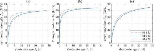
Table 1. Values of s_E and $s_{E_c}$ for three typical cement types [42]; and of uniaxial compressive strength reached 28 days after production, $f_{c,28\mathrm{d}},$ for three typical shotcrete strength classes.

cement type	sE	$s_{E_c}$	strength class	$f_{c,28\mathrm{d}}$
CEM II/A-M(S-L) 42.5 N	0.22	0.62	SpC 20/25	20 MPa
CEM II/A-S 42.5 R	0.18	0.61	SpC 25/30	25 MPa
CEM I 52.5 R	0.09	0.50	SpC 30/37	30 MPa

The creep modulus E_c is available from isothermal creep tests performed at a temperature of 20 centigrades [42], namely in the format (14) $$E_c(t)=E_{c,28\mathrm{d}}{\left\{\hspace{0.17em}\mathrm{\text{exp}}\hspace{0.17em}\mathrm{}\left[s_{E_c}\left(1-\sqrt{\frac{28\hspace{0.17em}\text{days}}{t}}\right)\right]\right\}}^{0.5},$$(14) with the creep modulus of concrete reached 28 days after production $E_{c,28\mathrm{d}},$ estimated through (15) $$E_{c,28\mathrm{d}}=51.9\hspace{0.17em}\text{GPa}\times {\alpha }^2{\left(\frac{f_{c,28\mathrm{d}}}{f_c^{*}}\right)}^{2/3},$$(15) and with the creep modulus evolution parameter $s_{E_c},$ see again Table 1 for typical values concerning shotcrete, and Figure 1(c) for an illustration of the creep modulus evolution.

We are left with quantifying the affinity factor η, which is linked to the stress-over-strength ratio or utilization degree $\mathcal{U} (>0),$ via [21] (16) $$\eta =1+2 {\mathcal{U}}^4.$$(16)

In order to define $\mathcal{U}$ in a three-dimensional setting, we adopt a Drucker-Prager strength criterion [45] specified for the stress components occurring in the tunnel shell, so that (17) $$\begin{array}{lll}\mathcal{U}(r,\phi ,t)& =& +\frac{{\alpha }_{\mathit{\text{DP}}}}{k_{\mathit{\text{DP}}}}[{\sigma }_{\phi \phi }(r,\phi ,t)+{\sigma }_{\mathit{\text{zz}}}(r,\phi ,t)]+\frac{1}{k_{\mathit{\text{DP}}}}\left\{\frac{2}{3}\right[{({\sigma }_{\phi \phi }(r,\phi ,t))}^2\\ & & -{\sigma }_{\phi \phi }(r,\phi ,t){\sigma }_{\mathit{\text{zz}}}(r,\phi ,t)+{({\sigma }_{\mathit{\text{zz}}}(r,\phi ,t))}^2]{\}}^{1/2},\end{array}$$(17) with parameters α_DP and k_DP being related to the uniaxial and biaxial compressive strengths of shotcrete, denoted as f_c and f_b, (18) $${\alpha }_{\mathit{\text{DP}}}=\sqrt{\frac{2}{3}}\frac{\kappa -1}{2\kappa -1},k_{\mathit{\text{DP}}}=\sqrt{\frac{2}{3}}\left[1-\frac{\kappa -1}{2\kappa -1}\right]f_c,$$(18) where the strength ratio $\kappa =f_b/f_c=1.15$ follows from classical mechanical experiments [46]. In analogy to the relations for elasticity and creep, which are given in Eqs. (12)(12) $$E(t)=E_{28\mathrm{d}}{\left\{\hspace{0.17em}\mathrm{\text{exp}}\hspace{0.17em}\mathrm{}\left[s_E\left(1-\sqrt{\frac{28\hspace{0.17em}\text{days}}{t}} \right)\mathrm{}\right]\right\}}^{0.5},$$(12) and (14)(14) $$E_c(t)=E_{c,28\mathrm{d}}{\left\{\hspace{0.17em}\mathrm{\text{exp}}\hspace{0.17em}\mathrm{}\left[s_{E_c}\left(1-\sqrt{\frac{28\hspace{0.17em}\text{days}}{t}}\right)\right]\right\}}^{0.5},$$(14) , the temporal evolution of the uniaxial strength of shotcrete under isothermal conditions at 20 centigrade can be approximated according to relevant standards [44], (19) $$f_c(t)=f_{c,28\mathrm{d}}\hspace{0.17em}\mathrm{\text{exp}}\hspace{0.17em}\mathrm{}\left[s_E\left(1-\sqrt{\frac{28\hspace{0.17em}\text{days}}{t}} \right)\right],$$(19) see Table 1 for typical values, and Figure 1(a) for a graphical illustration.

2.3. Spatial distributions across tunnel segment, of displacements, generator rotations, normal forces, and bending moments, as functions of ground pressure and impost force

In the framework of thin shell theory, force quantities of classical 3D continuum mechanics, such as Cauchy stress and traction forces, are homogenized into stress and force resultants, with the latter performing power on virtual velocities and virtual angular velocities associated with rigid body movements of the shell generator lines [14, 47, 48]. More specifically, the normal stress components ${\sigma }_{\phi \phi }$ and σ_zz are integrated over the shell generator lines, along the thickness h of the cylindrical shell with radius R, see Figure 2. This yields circumferential normal forces (per length measured in the tunnel driving direction), reading as [14, 49, 50] (20) $$n_{\phi }(\phi )=\underset{R-h/2}{\overset{R+h/2}{\int }}{\sigma }_{\phi \phi }(r,\phi )\mathrm{d}r,$$(20) as well as bending moments (per length measured in the tunnel driving direction), reading as (21) $$m_z(\phi )=\underset{R-h/2}{\overset{R+h/2}{\int }}{\sigma }_{\phi \phi }(r,\phi )\times (r-R)\mathrm{d}r.$$(21)

Figure 2. Illustration of slender arch-like tunnel cross section with radius R and thickness h, global Cartesian base frame ${\mathbf{e}}_x,{\mathbf{e}}_y,{\mathbf{e}}_z,$ and local polar base frames ${\mathbf{e}}_r(\phi ),{\mathbf{e}}_{\phi }(\phi ),{\mathbf{e}}_z;$ the latter is indicated at the left and right impost of the arch-like tunnel cross section, labeled by polar angles ${\phi }_{\mathit{\text{RI}}}$ and ${\phi }_{\mathit{\text{LI}}},$ reproduced from [14], copyright by the authors.

The corresponding circumferential normal traction forces $T_{\phi },$ acting at the imposts on surfaces with normals n oriented in circumferential direction, are summed up over the shell thickness as well, yielding impost forces at both ends of the tunnel segments, in the form [14] (22) $$\begin{array}{ccc}{N}_p& =& +\underset{R-h/2}{\overset{R+h/2}{\int }}{T}_{\phi }[r,{\phi }_{\mathit{\text{RI}}};\mathbf{n}=-{\mathbf{e}}_{\phi }({\phi }_{\mathit{\text{RI}}})]\mathrm{d}r\\ & =& -\underset{R-h/2}{\overset{R+h/2}{\int }}{\sigma }_{\phi \phi }(r,{\phi }_{\mathit{\text{RI}}})\mathrm{d}r=-n_{\phi }({\phi }_{\mathit{\text{RI}}})\\ & =& -\underset{R-h/2}{\overset{R+h/2}{\int }}{T}_{\phi }[r,{\phi }_{\mathit{\text{LI}}};\mathbf{n}=+{\mathbf{e}}_{\phi }({\phi }_{\mathit{\text{LI}}})]\mathrm{d}r\\ & =& -\underset{R-h/2}{\overset{R+h/2}{\int }}{\sigma }_{\phi \phi }(r,{\phi }_{\mathit{\text{LI}}})\mathrm{d}r=-n_{\phi }({\phi }_{\mathit{\text{LI}}}).\end{array}$$(22)

Furthermore, following classical terminology in tunnel engineering [51, 52], the radial normal traction forces T_r transferred from the ground onto the tunnel shell are referred to as ground pressure, (23) $$\begin{array}{ccc}{G}_p(\phi )& =& -T_r[r=R+h/2,\phi ;\mathbf{n}=+{\mathbf{e}}_r(\phi )].\end{array}$$(23)

Thereby, G_p is approximated as the superposition of four cubic polynomials, in the format (24) $$\begin{array}{lll}{G}_p(\overline{\phi })& =& +A_1(\overline{\phi })\hspace{0.17em}{G}_{p,1}+A_2(\overline{\phi })\hspace{0.17em}{G}_{p,2}+A_3(\overline{\phi })\hspace{0.17em}{G}_{p,3}+A_4(\overline{\phi })\hspace{0.17em}{G}_{p,4},\end{array}$$(24) with the cubic polynomials A_i, $i=1,2,3,4,$ reading as (25) $$\begin{array}{ccc}{A}_1(\overline{\phi })& =& 1-\frac{11\overline{\phi }}{2\Delta \phi }+\frac{9{\overline{\phi }}^2}{{(\Delta \phi )}^2}-\frac{9{\overline{\phi }}^3}{2{(\Delta \phi )}^3},\\ A_2(\overline{\phi })& =& \frac{9\overline{\phi }}{\Delta \phi }-\frac{45{\overline{\phi }}^2}{2{(\Delta \phi )}^2}+\frac{27{\overline{\phi }}^3}{2{(\Delta \phi )}^3},\\ A_3(\overline{\phi })& =& -\frac{9\overline{\phi }}{2\Delta \phi }+\frac{18{\overline{\phi }}^2}{{(\Delta \phi )}^2}-\frac{27{\overline{\phi }}^3}{2{(\Delta \phi )}^3},\\ A_4(\overline{\phi })& =& \frac{\overline{\phi }}{\Delta \phi }-\frac{9{\overline{\phi }}^2}{2{(\Delta \phi )}^2}+\frac{9{\overline{\phi }}^3}{2{(\Delta \phi )}^3},\end{array}$$(25) whereby $\Delta \phi ={\phi }_{\mathit{\text{LI}}}-{\phi }_{\mathit{\text{RI}}}$ denotes the opening angle of the tunnel shell, and $\overline{\phi }$ denotes the inclined azimuthal coordinate, measured from the right impost of the arch-like tunnel cross section, see Figure 3 for the example of the Sieberg tunnel.

Figure 3. Cross section of the Sieberg tunnel with focus on the top heading: definition of ${\mathbf{e}}_x$-${\mathbf{e}}_y$ and ${\mathbf{e}}_r(\overline{\phi })$-${\mathbf{e}}_{\phi }(\overline{\phi })$ coordinate frames, geometric properties and locations of measurement points MP1, MP2, and MP3, reproduced from [14], copyright by the authors.

In Eq. (24)(24) $$\begin{array}{lll}{G}_p(\overline{\phi })& =& +A_1(\overline{\phi })\hspace{0.17em}{G}_{p,1}+A_2(\overline{\phi })\hspace{0.17em}{G}_{p,2}+A_3(\overline{\phi })\hspace{0.17em}{G}_{p,3}+A_4(\overline{\phi })\hspace{0.17em}{G}_{p,4},\end{array}$$(24) , $G_{p,1}$ is the ground pressure at position $\overline{\phi }=0,$ i.e. at the right impost, $G_{p,2}$ is the ground pressure at position $\overline{\phi }=\Delta \phi /3,G_{p,3}$ is the ground pressure at position $\overline{\phi }=2\Delta \phi /3,$ and $G_{p,4}$ is the ground pressure at position $\overline{\phi }=\Delta \phi .$ The corresponding displacement distributions evolving over time can be given in the following rate format [14], (26) $$\begin{array}{c}+{\dot{u}}_r^M(\overline{\phi },t)-{\dot{u}}_{\phi ,\mathit{\text{RI}}}^M(t)\hspace{0.17em}\mathrm{\text{sin}}\hspace{0.17em}(\overline{\phi })-{\dot{u}}_{r,\mathit{\text{RI}}}^M(t)\hspace{0.17em}\mathrm{\text{cos}}\hspace{0.17em}(\overline{\phi })+R {\dot{\theta }}_{z,\mathit{\text{RI}}}^M(t)\hspace{0.17em}\mathrm{\text{sin}}\hspace{0.17em}(\overline{\phi })\hfill \\ =+{\mathcal{I}}_{N\to r}(\overline{\phi })[{\int }_0^t\frac{\partial J^{\sigma }}{\partial t}(\xi (t),\eta ({\overline{\sigma }}_{\phi \phi }(t),{\overline{\sigma }}_{\mathit{\text{zz}}}(t)),t-\tau ){\dot{N}}_p(\tau )\mathrm{d}\tau ]\hfill \\ +\sum _{i=1}^4\{{\mathcal{I}}_{i\to r}(\overline{\phi })[{\int }_0^t\frac{\partial J^{\sigma }}{\partial t}(\xi (t),\eta ({\overline{\sigma }}_{\phi \phi }(t),{\overline{\sigma }}_{\mathit{\text{zz}}}(t)),t-\tau ){\dot{G}}_{p,i}(\tau )\mathrm{d}\tau \left]\right\},\hfill \end{array}$$(26) (27) $$\begin{array}{c}+{\dot{u}}_{\phi }^M(\overline{\phi },t)-{\dot{u}}_{\phi ,\mathit{\text{RI}}}^M(t)\hspace{0.17em}\mathrm{\text{cos}}\hspace{0.17em}(\overline{\phi })+{\dot{u}}_{r,\mathit{\text{RI}}}^M(t)\hspace{0.17em}\mathrm{\text{sin}}\hspace{0.17em}(\overline{\phi })+R {\dot{\theta }}_{z,\mathit{\text{RI}}}^M(t)\{\mathrm{\text{cos}}(\overline{\phi })-1\}\hfill \\ =+{\mathcal{I}}_{N\to \phi }(\overline{\phi })[{\int }_0^t\frac{\partial J^{\sigma }}{\partial t}(\xi (t),\eta ({\overline{\sigma }}_{\phi \phi }(t),{\overline{\sigma }}_{\mathit{\text{zz}}}(t)),t-\tau ){\dot{N}}_p(\tau )\mathrm{d}\tau ]\hfill \\ +\sum _{i=1}^4\{{\mathcal{I}}_{i\to \phi }(\overline{\phi })[{\int }_0^t\frac{\partial J^{\sigma }}{\partial t}(\xi (t),\eta ({\overline{\sigma }}_{\phi \phi }(t),{\overline{\sigma }}_{\mathit{\text{zz}}}(t)),t-\tau ){\dot{G}}_{p,i}(\tau )\mathrm{d}\tau \left]\right\},\hfill \end{array}$$(27) while the temporally evolving distributions of the shell generator rotations read as [14] (28) $$\begin{array}{c}+{\dot{\theta }}_z^M(\overline{\phi },t)-{\dot{\theta }}_{z,\mathit{\text{RI}}}^M(t)\hfill \\ =+{\mathcal{I}}_{N\to z}(\overline{\phi })[{\int }_0^t\frac{\partial J^{\sigma }}{\partial t}(\xi (t),\eta ({\overline{\sigma }}_{\phi \phi }(t),{\overline{\sigma }}_{\mathit{\text{zz}}}(t)),t-\tau ){\dot{N}}_p(\tau )\mathrm{d}\tau ]\hfill \\ +\sum _{i=1}^4\{{\mathcal{I}}_{i\to z}(\overline{\phi })[{\int }_0^t\frac{\partial J^{\sigma }}{\partial t}(\xi (t),\eta ({\overline{\sigma }}_{\phi \phi }(t),{\overline{\sigma }}_{\mathit{\text{zz}}}(t)),t-\tau ){\dot{G}}_{p,i}(\tau )\mathrm{d}\tau \left]\right\}.\hfill \end{array}$$(28)

In Eqs. (26)(26) $$\begin{array}{c}+{\dot{u}}_r^M(\overline{\phi },t)-{\dot{u}}_{\phi ,\mathit{\text{RI}}}^M(t)\hspace{0.17em}\mathrm{\text{sin}}\hspace{0.17em}(\overline{\phi })-{\dot{u}}_{r,\mathit{\text{RI}}}^M(t)\hspace{0.17em}\mathrm{\text{cos}}\hspace{0.17em}(\overline{\phi })+R {\dot{\theta }}_{z,\mathit{\text{RI}}}^M(t)\hspace{0.17em}\mathrm{\text{sin}}\hspace{0.17em}(\overline{\phi })\hfill \\ =+{\mathcal{I}}_{N\to r}(\overline{\phi })[{\int }_0^t\frac{\partial J^{\sigma }}{\partial t}(\xi (t),\eta ({\overline{\sigma }}_{\phi \phi }(t),{\overline{\sigma }}_{\mathit{\text{zz}}}(t)),t-\tau ){\dot{N}}_p(\tau )\mathrm{d}\tau ]\hfill \\ +\sum _{i=1}^4\{{\mathcal{I}}_{i\to r}(\overline{\phi })[{\int }_0^t\frac{\partial J^{\sigma }}{\partial t}(\xi (t),\eta ({\overline{\sigma }}_{\phi \phi }(t),{\overline{\sigma }}_{\mathit{\text{zz}}}(t)),t-\tau ){\dot{G}}_{p,i}(\tau )\mathrm{d}\tau \left]\right\},\hfill \end{array}$$(26) and (27)(27) $$\begin{array}{c}+{\dot{u}}_{\phi }^M(\overline{\phi },t)-{\dot{u}}_{\phi ,\mathit{\text{RI}}}^M(t)\hspace{0.17em}\mathrm{\text{cos}}\hspace{0.17em}(\overline{\phi })+{\dot{u}}_{r,\mathit{\text{RI}}}^M(t)\hspace{0.17em}\mathrm{\text{sin}}\hspace{0.17em}(\overline{\phi })+R {\dot{\theta }}_{z,\mathit{\text{RI}}}^M(t)\{\mathrm{\text{cos}}(\overline{\phi })-1\}\hfill \\ =+{\mathcal{I}}_{N\to \phi }(\overline{\phi })[{\int }_0^t\frac{\partial J^{\sigma }}{\partial t}(\xi (t),\eta ({\overline{\sigma }}_{\phi \phi }(t),{\overline{\sigma }}_{\mathit{\text{zz}}}(t)),t-\tau ){\dot{N}}_p(\tau )\mathrm{d}\tau ]\hfill \\ +\sum _{i=1}^4\{{\mathcal{I}}_{i\to \phi }(\overline{\phi })[{\int }_0^t\frac{\partial J^{\sigma }}{\partial t}(\xi (t),\eta ({\overline{\sigma }}_{\phi \phi }(t),{\overline{\sigma }}_{\mathit{\text{zz}}}(t)),t-\tau ){\dot{G}}_{p,i}(\tau )\mathrm{d}\tau \left]\right\},\hfill \end{array}$$(27) , ${\dot{u}}_r^M$ and ${\dot{u}}_{\phi }^M$ denote the radial and circumferential displacement rates of the midsurface of the tunnel shell segment; and in Eq. (28)(28) $$\begin{array}{c}+{\dot{\theta }}_z^M(\overline{\phi },t)-{\dot{\theta }}_{z,\mathit{\text{RI}}}^M(t)\hfill \\ =+{\mathcal{I}}_{N\to z}(\overline{\phi })[{\int }_0^t\frac{\partial J^{\sigma }}{\partial t}(\xi (t),\eta ({\overline{\sigma }}_{\phi \phi }(t),{\overline{\sigma }}_{\mathit{\text{zz}}}(t)),t-\tau ){\dot{N}}_p(\tau )\mathrm{d}\tau ]\hfill \\ +\sum _{i=1}^4\{{\mathcal{I}}_{i\to z}(\overline{\phi })[{\int }_0^t\frac{\partial J^{\sigma }}{\partial t}(\xi (t),\eta ({\overline{\sigma }}_{\phi \phi }(t),{\overline{\sigma }}_{\mathit{\text{zz}}}(t)),t-\tau ){\dot{G}}_{p,i}(\tau )\mathrm{d}\tau \left]\right\}.\hfill \end{array}$$(28) , ${\dot{\theta }}_z^M$ stands for the rate of the rotational angle of the shell generator lying perpendicular to the midsurface of the tunnel segment. This follows the kinematic reasoning given in [13, 14, 53], so that the introduction of generator rotations in the context of a right-handed base frame implies that (29) $${\theta }_z^M=-\frac{1}{R}\frac{\mathrm{d}{u}_r^M}{\mathrm{d}\phi }+\frac{u_{\phi }^M}{R}.$$(29)

Furthermore, in Eqs. (26)(26) $$\begin{array}{c}+{\dot{u}}_r^M(\overline{\phi },t)-{\dot{u}}_{\phi ,\mathit{\text{RI}}}^M(t)\hspace{0.17em}\mathrm{\text{sin}}\hspace{0.17em}(\overline{\phi })-{\dot{u}}_{r,\mathit{\text{RI}}}^M(t)\hspace{0.17em}\mathrm{\text{cos}}\hspace{0.17em}(\overline{\phi })+R {\dot{\theta }}_{z,\mathit{\text{RI}}}^M(t)\hspace{0.17em}\mathrm{\text{sin}}\hspace{0.17em}(\overline{\phi })\hfill \\ =+{\mathcal{I}}_{N\to r}(\overline{\phi })[{\int }_0^t\frac{\partial J^{\sigma }}{\partial t}(\xi (t),\eta ({\overline{\sigma }}_{\phi \phi }(t),{\overline{\sigma }}_{\mathit{\text{zz}}}(t)),t-\tau ){\dot{N}}_p(\tau )\mathrm{d}\tau ]\hfill \\ +\sum _{i=1}^4\{{\mathcal{I}}_{i\to r}(\overline{\phi })[{\int }_0^t\frac{\partial J^{\sigma }}{\partial t}(\xi (t),\eta ({\overline{\sigma }}_{\phi \phi }(t),{\overline{\sigma }}_{\mathit{\text{zz}}}(t)),t-\tau ){\dot{G}}_{p,i}(\tau )\mathrm{d}\tau \left]\right\},\hfill \end{array}$$(26) – (28)(28) $$\begin{array}{c}+{\dot{\theta }}_z^M(\overline{\phi },t)-{\dot{\theta }}_{z,\mathit{\text{RI}}}^M(t)\hfill \\ =+{\mathcal{I}}_{N\to z}(\overline{\phi })[{\int }_0^t\frac{\partial J^{\sigma }}{\partial t}(\xi (t),\eta ({\overline{\sigma }}_{\phi \phi }(t),{\overline{\sigma }}_{\mathit{\text{zz}}}(t)),t-\tau ){\dot{N}}_p(\tau )\mathrm{d}\tau ]\hfill \\ +\sum _{i=1}^4\{{\mathcal{I}}_{i\to z}(\overline{\phi })[{\int }_0^t\frac{\partial J^{\sigma }}{\partial t}(\xi (t),\eta ({\overline{\sigma }}_{\phi \phi }(t),{\overline{\sigma }}_{\mathit{\text{zz}}}(t)),t-\tau ){\dot{G}}_{p,i}(\tau )\mathrm{d}\tau \left]\right\}.\hfill \end{array}$$(28) , ${\dot{u}}_{r,\mathit{\text{RI}}}^M,{\dot{u}}_{\phi ,\mathit{\text{RI}}}^M,$ and ${\dot{\theta }}_{z,\mathit{\text{RI}}}^M$ stand for the aforementioned quantities at the right impost of the shell, ${\dot{N}}_p$ and ${\dot{G}}_{p,i}$ stand for the rates of the impost force and ground pressure values at the positions $\overline{\phi }=(i-1)\Delta \phi /3,{\overline{\sigma }}_{\phi \phi }$ and ${\overline{\sigma }}_{\mathit{\text{zz}}}$ stand for the circumferential and axial normal stresses averaged over the shell thickness, and the influence functions $\mathcal{I}$ are defined in Appendix B: In more detail, the force-to-displacement influence functions ${\mathcal{I}}_{N\to r}$ and ${\mathcal{I}}_{N\to \phi }$ are defined through Eqs. (B1)(B1) $$\begin{array}{lll}{\mathcal{I}}_{N\to r}(\overline{\phi })& =& \{1-{\nu }^2\}\{\frac{12R^3}{h^3}[\mathrm{\text{cos}}\hspace{0.17em}(\overline{\phi })-1]+[\frac{R}{2h}+\frac{6R^3}{h^3}\left]\right[\frac{\overline{\phi }\hspace{0.17em}\mathrm{\text{cos}}\hspace{0.17em}(\overline{\phi })}{\hspace{0.17em}\mathrm{\text{tan}}\hspace{0.17em}(\Delta \phi )}\\ & & +\overline{\phi }\hspace{0.17em}\mathrm{\text{sin}}\hspace{0.17em}(\overline{\phi })-\frac{\hspace{0.17em}\mathrm{\text{sin}}\hspace{0.17em}(\overline{\phi })}{\hspace{0.17em}\mathrm{\text{tan}}\hspace{0.17em}(\Delta \phi )}+\frac{\hspace{0.17em}\mathrm{\text{sin}}\hspace{0.17em}(\overline{\phi })}{\hspace{0.17em}\mathrm{\text{sin}}\hspace{0.17em}(\Delta \phi )}-\frac{\overline{\phi }\hspace{0.17em}\mathrm{\text{cos}}\hspace{0.17em}(\overline{\phi })}{\hspace{0.17em}\mathrm{\text{sin}}\hspace{0.17em}(\Delta \phi )}\left]\right\},\end{array}$$(B1) and (B6)(B6) $$\begin{array}{lll}{\mathcal{I}}_{N\to \phi }(\overline{\phi })& =& \{1-{\nu }^2\}\{[\frac{R}{2h}+\frac{6R^3}{h^3}][\overline{\phi }\hspace{0.17em}\mathrm{\text{cos}}\hspace{0.17em}(\overline{\phi })-3\hspace{0.17em}\mathrm{\text{sin}}\hspace{0.17em}(\overline{\phi })-\frac{\overline{\phi }\hspace{0.17em}\mathrm{\text{sin}}\hspace{0.17em}(\overline{\phi })}{\hspace{0.17em}\mathrm{\text{tan}}\hspace{0.17em}(\Delta \phi )}+\frac{\overline{\phi }\hspace{0.17em}\mathrm{\text{sin}}\hspace{0.17em}(\overline{\phi })}{\hspace{0.17em}\mathrm{\text{sin}}\hspace{0.17em}(\Delta \phi )}]\\ & & +\frac{R}{h}[2\hspace{0.17em}\mathrm{\text{sin}}\hspace{0.17em}(\overline{\phi })]+\frac{12R^3}{h^3}[\overline{\phi }-\frac{\hspace{0.17em}\mathrm{\text{cos}}\hspace{0.17em}(\overline{\phi })-1}{\hspace{0.17em}\mathrm{\text{tan}}\hspace{0.17em}(\Delta \phi )}+\frac{\hspace{0.17em}\mathrm{\text{cos}}\hspace{0.17em}(\overline{\phi })-1}{\hspace{0.17em}\mathrm{\text{sin}}\hspace{0.17em}(\Delta \phi )}]\},\end{array}$$(B6) , the pressure-to-displacement influence functions ${\mathcal{I}}_{i\to r}$ and ${\mathcal{I}}_{i\to \phi },\text{\hspace{0.17em}with}i=1,\hspace{0.17em}2,\hspace{0.17em}3,\hspace{0.17em}4$ are defined through Eqs. (B2)(B2) $$\begin{array}{lll}{\mathcal{I}}_{1\to r}(\overline{\phi })& =& \{1-{\nu }^2\}\left\{\right[\frac{R^2}{h}+\frac{12R^4}{h^3}\left]\right[-1-\frac{54\overline{\phi }}{{(\Delta \phi )}^3}+\frac{9{\overline{\phi }}^3}{2{(\Delta \phi )}^3}+\frac{36}{{(\Delta \phi )}^2}\\ -\frac{9{\overline{\phi }}^2}{{(\Delta \phi )}^2}+\frac{11\overline{\phi }}{2\Delta \phi }-\frac{36\hspace{0.17em}\mathrm{\text{cos}}\hspace{0.17em}(\overline{\phi })}{{(\Delta \phi )}^2}+\frac{\overline{\phi }\hspace{0.17em}\mathrm{\text{cos}}\hspace{0.17em}(\overline{\phi })}{2\hspace{0.17em}\mathrm{\text{tan}}\hspace{0.17em}(\Delta \phi )}\hfill \\ & -\frac{9\overline{\phi }\hspace{0.17em}\mathrm{\text{cos}}\hspace{0.17em}(\overline{\phi })}{{(\Delta \phi )}^2\hspace{0.17em}\mathrm{\text{tan}}\hspace{0.17em}(\Delta \phi )}+\hspace{0.17em}\mathrm{\text{cos}}\hspace{0.17em}(\overline{\phi })-\frac{9\overline{\phi }\hspace{0.17em}\mathrm{\text{cos}}\hspace{0.17em}(\overline{\phi })}{2{(\Delta \phi )}^2\hspace{0.17em}\mathrm{\text{sin}}\hspace{0.17em}(\Delta \phi )}\\ & & +\frac{\overline{\phi }\hspace{0.17em}\mathrm{\text{sin}}\hspace{0.17em}(\overline{\phi })}{2}+\frac{54\hspace{0.17em}\mathrm{\text{sin}}\hspace{0.17em}(\overline{\phi })}{{(\Delta \phi )}^3}-\frac{9\overline{\phi }\hspace{0.17em}\mathrm{\text{sin}}\hspace{0.17em}(\overline{\phi })}{{(\Delta \phi )}^2}-\frac{11\hspace{0.17em}\mathrm{\text{sin}}\hspace{0.17em}(\overline{\phi })}{2\Delta \phi }\\ & & -\frac{\hspace{0.17em}\mathrm{\text{sin}}\hspace{0.17em}(\overline{\phi })}{2\hspace{0.17em}\mathrm{\text{tan}}\hspace{0.17em}(\Delta \phi )}+\frac{9\hspace{0.17em}\mathrm{\text{sin}}\hspace{0.17em}(\overline{\phi })}{{(\Delta \phi )}^2\hspace{0.17em}\mathrm{\text{tan}}\hspace{0.17em}(\Delta \phi )}+\frac{9\hspace{0.17em}\mathrm{\text{sin}}\hspace{0.17em}(\overline{\phi })}{2{(\Delta \phi )}^2\hspace{0.17em}\mathrm{\text{sin}}\hspace{0.17em}(\Delta \phi )}\left]\right\},\end{array}$$(B2) – (B5)(B5) $$\begin{array}{lll}{\mathcal{I}}_{4\to r}(\overline{\phi })& \mathrm{}\mathrm{}=\mathrm{}\mathrm{}& \{1-{\nu }^2\}\{[\frac{R^2}{h}+\frac{12R^4}{h^3}]\mathrm{}[\frac{54\overline{\phi }}{{(\Delta \phi )}^3}-\frac{9{\overline{\phi }}^3}{2{(\Delta \phi )}^3}-\frac{18}{{(\Delta \phi )}^2}-\frac{\overline{\phi }}{\Delta \phi }\\ & & +\frac{9{\overline{\phi }}^2}{2{(\Delta \phi )}^2}+\frac{18\hspace{0.17em}\mathrm{\text{cos}}\hspace{0.17em}(\overline{\phi })}{{(\Delta \phi )}^2}+\frac{9\overline{\phi }\hspace{0.17em}\mathrm{\text{cos}}\hspace{0.17em}(\overline{\phi })}{2{(\Delta \phi )}^2\hspace{0.17em}\mathrm{\text{tan}}\hspace{0.17em}(\Delta \phi )}-\frac{54\hspace{0.17em}\mathrm{\text{sin}}\hspace{0.17em}(\overline{\phi })}{{(\Delta \phi )}^3}\\ & & +\frac{9\overline{\phi }\hspace{0.17em}\mathrm{\text{cos}}\hspace{0.17em}(\overline{\phi })}{{(\Delta \phi )}^2\hspace{0.17em}\mathrm{\text{sin}}\hspace{0.17em}(\Delta \phi )}+\frac{9\overline{\phi }\hspace{0.17em}\mathrm{\text{sin}}\hspace{0.17em}(\overline{\phi })}{2{(\Delta \phi )}^2}-\frac{\overline{\phi }\hspace{0.17em}\mathrm{\text{cos}}\hspace{0.17em}(\overline{\phi })}{2\hspace{0.17em}\mathrm{\text{sin}}\hspace{0.17em}(\Delta \phi )}+\frac{\hspace{0.17em}\mathrm{\text{sin}}\hspace{0.17em}(\overline{\phi })}{\Delta \phi }\\ & & -\frac{9\hspace{0.17em}\mathrm{\text{sin}}\hspace{0.17em}(\overline{\phi })}{2{(\Delta \phi )}^2\hspace{0.17em}\mathrm{\text{tan}}\hspace{0.17em}(\Delta \phi )}+\frac{\hspace{0.17em}\mathrm{\text{sin}}\hspace{0.17em}(\overline{\phi })}{2\hspace{0.17em}\mathrm{\text{sin}}\hspace{0.17em}(\Delta \phi )}-\frac{9\hspace{0.17em}\mathrm{\text{sin}}\hspace{0.17em}(\overline{\phi })}{{(\Delta \phi )}^2\hspace{0.17em}\mathrm{\text{sin}}\hspace{0.17em}(\Delta \phi )}]\}.\end{array}$$(B5) and Eqs. (B7)(B7) $$\begin{array}{lll}{\mathcal{I}}_{1\to \phi }(\overline{\phi })& =& \{1-{\nu }^2\}\{[\frac{R^2}{h}+\frac{12R^4}{h^3}][-\frac{54-54\hspace{0.17em}\mathrm{\text{cos}}\hspace{0.17em}(\overline{\phi })}{{(\Delta \phi )}^3}+\frac{11-11\hspace{0.17em}\mathrm{\text{cos}}\hspace{0.17em}(\overline{\phi })}{2\Delta \phi }\\ & & +\frac{\overline{\phi }\hspace{0.17em}\mathrm{\text{cos}}\hspace{0.17em}(\overline{\phi })}{2}-\frac{9\overline{\phi }\hspace{0.17em}\mathrm{\text{cos}}\hspace{0.17em}(\overline{\phi })}{{(\Delta \phi )}^2}-\frac{\overline{\phi }\hspace{0.17em}\mathrm{\text{sin}}\hspace{0.17em}(\overline{\phi })}{2\hspace{0.17em}\mathrm{\text{tan}}\hspace{0.17em}(\Delta \phi )}+\frac{9\overline{\phi }\hspace{0.17em}\mathrm{\text{sin}}\hspace{0.17em}(\overline{\phi })}{{(\Delta \phi )}^2\hspace{0.17em}\mathrm{\text{tan}}\hspace{0.17em}(\Delta \phi )}\\ & & +\frac{9\overline{\phi }\hspace{0.17em}\mathrm{\text{sin}}\hspace{0.17em}(\overline{\phi })}{2{(\Delta \phi )}^2\hspace{0.17em}\mathrm{\text{sin}}\hspace{0.17em}(\Delta \phi )}]+\frac{R^2}{h}[+\frac{27{\overline{\phi }}^2}{2{(\Delta \phi )}^3}-\frac{18\overline{\phi }}{{(\Delta \phi )}^2}\\ & & -\frac{\hspace{0.17em}\mathrm{\text{sin}}\hspace{0.17em}(\overline{\phi })}{2}+\frac{27\hspace{0.17em}\mathrm{\text{sin}}\hspace{0.17em}(\overline{\phi })}{{(\Delta \phi )}^2}]+\frac{12R^4}{h^3}[\frac{3{\overline{\phi }}^3}{{(\Delta \phi )}^2}-\frac{9{\overline{\phi }}^4}{8{(\Delta \phi )}^3}\\ & & -\frac{11{\overline{\phi }}^2}{4\Delta \phi }+\frac{27{\overline{\phi }}^2}{{(\Delta \phi )}^3}-\frac{36\overline{\phi }}{{(\Delta \phi )}^2}-\frac{3\hspace{0.17em}\mathrm{\text{sin}}\hspace{0.17em}(\overline{\phi })}{2}+\frac{45\hspace{0.17em}\mathrm{\text{sin}}\hspace{0.17em}(\overline{\phi })}{{(\Delta \phi )}^2}\\ & & -\frac{9-9\hspace{0.17em}\mathrm{\text{cos}}\hspace{0.17em}(\overline{\phi })}{{(\Delta \phi )}^2\hspace{0.17em}\mathrm{\text{sin}}\hspace{0.17em}(\Delta \phi )}+\frac{1-\hspace{0.17em}\mathrm{\text{cos}}\hspace{0.17em}(\overline{\phi })}{\hspace{0.17em}\mathrm{\text{tan}}\hspace{0.17em}(\Delta \phi )}-\frac{18-18\hspace{0.17em}\mathrm{\text{cos}}\hspace{0.17em}(\overline{\phi })}{{(\Delta \phi )}^2\hspace{0.17em}\mathrm{\text{tan}}\hspace{0.17em}(\Delta \phi )}+\overline{\phi }]\},\end{array}$$(B7) – (B10)(B10) $$\begin{array}{lll}{\mathcal{I}}_{4\to \phi }(\overline{\phi })& =& \{1-{\nu }^2\}\{[\frac{R^2}{h}+\frac{12R^4}{h^3}][-\frac{1}{\Delta \phi }+\frac{54-54\hspace{0.17em}\mathrm{\text{cos}}\hspace{0.17em}(\overline{\phi })}{\Delta {\phi }^3}+\frac{\hspace{0.17em}\mathrm{\text{cos}}\hspace{0.17em}(\overline{\phi })}{\Delta \phi }\\ & & -\frac{9\overline{\phi }\hspace{0.17em}\mathrm{\text{sin}}\hspace{0.17em}(\overline{\phi })}{2\Delta {\phi }^2\hspace{0.17em}\mathrm{\text{tan}}\hspace{0.17em}(\Delta \phi )}+\frac{\overline{\phi }\hspace{0.17em}\mathrm{\text{sin}}\hspace{0.17em}(\overline{\phi })}{2\hspace{0.17em}\mathrm{\text{sin}}\hspace{0.17em}(\Delta \phi )}-\frac{9\overline{\phi }\hspace{0.17em}\mathrm{\text{sin}}\hspace{0.17em}(\overline{\phi })}{\Delta {\phi }^2\hspace{0.17em}\mathrm{\text{sin}}\hspace{0.17em}(\Delta \phi )}\\ & & +\frac{9\overline{\phi }\hspace{0.17em}\mathrm{\text{cos}}\hspace{0.17em}(\overline{\phi })}{2\Delta {\phi }^2}]+\frac{12R^4}{h^3}[-\frac{27{\overline{\phi }}^2}{\Delta {\phi }^3}+\frac{9{\overline{\phi }}^4}{8\Delta {\phi }^3}+\frac{18\overline{\phi }}{\Delta {\phi }^2}-\frac{3{\overline{\phi }}^3}{2\Delta {\phi }^2}\\ & & +\frac{{\overline{\phi }}^2}{2\Delta \phi }-\frac{45\hspace{0.17em}\mathrm{\text{sin}}\hspace{0.17em}(\overline{\phi })}{2\Delta {\phi }^2}+\frac{9-9\hspace{0.17em}\mathrm{\text{cos}}\hspace{0.17em}(\overline{\phi })}{\Delta {\phi }^2\hspace{0.17em}\mathrm{\text{tan}}\hspace{0.17em}(\Delta \phi )}-\frac{1-\hspace{0.17em}\mathrm{\text{cos}}\hspace{0.17em}(\overline{\phi })}{\hspace{0.17em}\mathrm{\text{sin}}\hspace{0.17em}(\Delta \phi )}\\ & & +\frac{18-18\hspace{0.17em}\mathrm{\text{cos}}\hspace{0.17em}(\overline{\phi })}{\Delta {\phi }^2\hspace{0.17em}\mathrm{\text{sin}}\hspace{0.17em}(\Delta \phi )}]+\frac{R^2}{h}[+\frac{9\overline{\phi }}{\Delta {\phi }^2}-\frac{27{\overline{\phi }}^2}{2\Delta {\phi }^3}-\frac{27\hspace{0.17em}\mathrm{\text{sin}}\hspace{0.17em}(\overline{\phi })}{2\Delta {\phi }^2}]\}.\end{array}$$(B10) , respectively, the force-to-rotation influence function ${\mathcal{I}}_{N\to z}$ is defined through Eq. (B11)(B11) $$\begin{array}{ccc}{\mathcal{I}}_{N\to z}(\overline{\phi })& =& \{1-{\nu }^2\}\{\frac{12R^2}{h^3}[\overline{\phi }-\frac{\hspace{0.17em}\mathrm{\text{cos}}\hspace{0.17em}(\overline{\phi })-1}{\hspace{0.17em}\mathrm{\text{tan}}\hspace{0.17em}(\Delta \phi )}-\frac{1-\hspace{0.17em}\mathrm{\text{cos}}\hspace{0.17em}(\overline{\phi })}{\hspace{0.17em}\mathrm{\text{sin}}\hspace{0.17em}(\Delta \phi )}-\hspace{0.17em}\mathrm{\text{sin}}\hspace{0.17em}(\overline{\phi })]\},\end{array}$$(B11) , and the pressure-to-rotation influence functions ${\mathcal{I}}_{i\to z},\text{with}i=1,\hspace{0.17em}2,\hspace{0.17em}3,\hspace{0.17em}4$ are defined through Eqs. (B12)(B12) $$\begin{array}{lll}{\mathcal{I}}_{1\to z}(\overline{\phi })& =& \{1-{\nu }^2\}\{\frac{12R^3}{h^3}[+\overline{\phi }+\frac{27{\overline{\phi }}^2}{2{(\Delta \phi )}^3}-\frac{9{\overline{\phi }}^4}{8{(\Delta \phi )}^3}-\frac{18\overline{\phi }}{{(\Delta \phi )}^2}\\ & & +\frac{3{\overline{\phi }}^3}{{(\Delta \phi )}^2}-\frac{11{\overline{\phi }}^2}{4\Delta \phi }+\frac{1-\hspace{0.17em}\mathrm{\text{cos}}\hspace{0.17em}(\overline{\phi })}{\hspace{0.17em}\mathrm{\text{tan}}\hspace{0.17em}(\Delta \phi )}-\hspace{0.17em}\mathrm{\text{sin}}\hspace{0.17em}(\overline{\phi })\\ & & +\frac{18\hspace{0.17em}\mathrm{\text{sin}}\hspace{0.17em}(\overline{\phi })}{{(\Delta \phi )}^2}-\frac{18-18\hspace{0.17em}\mathrm{\text{cos}}\hspace{0.17em}(\overline{\phi })}{{(\Delta \phi )}^2\hspace{0.17em}\mathrm{\text{tan}}\hspace{0.17em}(\Delta \phi )}-\frac{9-9\hspace{0.17em}\mathrm{\text{cos}}\hspace{0.17em}(\overline{\phi })}{{(\Delta \phi )}^2\hspace{0.17em}\mathrm{\text{sin}}\hspace{0.17em}(\Delta \phi )}]\},\end{array}$$(B12) – (B15)(B15) $$\begin{array}{lll}{\mathcal{I}}_{4\to z}(\overline{\phi })& =& \{1-{\nu }^2\}\{\frac{12R^3}{h^3}[-\frac{27{\overline{\phi }}^2}{2{(\Delta \phi )}^3}+\frac{9{\overline{\phi }}^4}{8{(\Delta \phi )}^3}+\frac{9\overline{\phi }}{{(\Delta \phi )}^2}\\ & & -\frac{3{\overline{\phi }}^3}{2{(\Delta \phi )}^2}+\frac{{\overline{\phi }}^2}{2\Delta \phi }-\frac{9\hspace{0.17em}\mathrm{\text{sin}}\hspace{0.17em}(\overline{\phi })}{{(\Delta \phi )}^2}\\ & & +\frac{9-9\hspace{0.17em}\mathrm{\text{cos}}\hspace{0.17em}(\overline{\phi })}{{(\Delta \phi )}^2\hspace{0.17em}\mathrm{\text{tan}}\hspace{0.17em}(\Delta \phi )}+\frac{18-18\hspace{0.17em}\mathrm{\text{cos}}\hspace{0.17em}(\overline{\phi })}{{(\Delta \phi )}^2\hspace{0.17em}\mathrm{\text{sin}}\hspace{0.17em}(\Delta \phi )}-\frac{1-\hspace{0.17em}\mathrm{\text{cos}}\hspace{0.17em}(\overline{\phi })}{\hspace{0.17em}\mathrm{\text{sin}}\hspace{0.17em}(\Delta \phi )}]\}.\end{array}$$(B15) .

After temporal discretization, which is described in more detail in Section 3, the relations (26)(26) $$\begin{array}{c}+{\dot{u}}_r^M(\overline{\phi },t)-{\dot{u}}_{\phi ,\mathit{\text{RI}}}^M(t)\hspace{0.17em}\mathrm{\text{sin}}\hspace{0.17em}(\overline{\phi })-{\dot{u}}_{r,\mathit{\text{RI}}}^M(t)\hspace{0.17em}\mathrm{\text{cos}}\hspace{0.17em}(\overline{\phi })+R {\dot{\theta }}_{z,\mathit{\text{RI}}}^M(t)\hspace{0.17em}\mathrm{\text{sin}}\hspace{0.17em}(\overline{\phi })\hfill \\ =+{\mathcal{I}}_{N\to r}(\overline{\phi })[{\int }_0^t\frac{\partial J^{\sigma }}{\partial t}(\xi (t),\eta ({\overline{\sigma }}_{\phi \phi }(t),{\overline{\sigma }}_{\mathit{\text{zz}}}(t)),t-\tau ){\dot{N}}_p(\tau )\mathrm{d}\tau ]\hfill \\ +\sum _{i=1}^4\{{\mathcal{I}}_{i\to r}(\overline{\phi })[{\int }_0^t\frac{\partial J^{\sigma }}{\partial t}(\xi (t),\eta ({\overline{\sigma }}_{\phi \phi }(t),{\overline{\sigma }}_{\mathit{\text{zz}}}(t)),t-\tau ){\dot{G}}_{p,i}(\tau )\mathrm{d}\tau \left]\right\},\hfill \end{array}$$(26) – (28)(28) $$\begin{array}{c}+{\dot{\theta }}_z^M(\overline{\phi },t)-{\dot{\theta }}_{z,\mathit{\text{RI}}}^M(t)\hfill \\ =+{\mathcal{I}}_{N\to z}(\overline{\phi })[{\int }_0^t\frac{\partial J^{\sigma }}{\partial t}(\xi (t),\eta ({\overline{\sigma }}_{\phi \phi }(t),{\overline{\sigma }}_{\mathit{\text{zz}}}(t)),t-\tau ){\dot{N}}_p(\tau )\mathrm{d}\tau ]\hfill \\ +\sum _{i=1}^4\{{\mathcal{I}}_{i\to z}(\overline{\phi })[{\int }_0^t\frac{\partial J^{\sigma }}{\partial t}(\xi (t),\eta ({\overline{\sigma }}_{\phi \phi }(t),{\overline{\sigma }}_{\mathit{\text{zz}}}(t)),t-\tau ){\dot{G}}_{p,i}(\tau )\mathrm{d}\tau \left]\right\}.\hfill \end{array}$$(28) allow for translation of displacement values measured at particular positions on the inner shell surface, into ground pressure and impost force values. The latter give access to normal forces and bending moments, via [14] (30) $$n_{\phi }(\overline{\phi })=+N_p {\mathcal{I}}_{N\to n}(\overline{\phi })-\sum _{i=1}^4[R G_{p,i} {\mathcal{I}}_{i\to n}(\overline{\phi })],$$(30) and (31) $$m_z(\overline{\phi })=+R N_p {\mathcal{I}}_{N\to m}(\overline{\phi })+\sum _{i=1}^4[R^2 G_{p,i} {\mathcal{I}}_{i\to n}(\overline{\phi })],$$(31) with the time-invariant influence functions $\mathcal{I}$ given as Eqs. (B16)(B16) $$\begin{array}{ccc}{\mathcal{I}}_{N\to n}(\overline{\phi })& =& +\hspace{0.17em}\mathrm{\text{cos}}\hspace{0.17em}(\overline{\phi })-\frac{\hspace{0.17em}\mathrm{\text{sin}}\hspace{0.17em}(\overline{\phi })}{\hspace{0.17em}\mathrm{\text{tan}}\hspace{0.17em}(\Delta \phi )}+\frac{\hspace{0.17em}\mathrm{\text{sin}}\hspace{0.17em}(\overline{\phi })}{\hspace{0.17em}\mathrm{\text{sin}}\hspace{0.17em}(\Delta \phi )},\end{array}$$(B16) – (B21)(B21) $$\begin{array}{ccc}{\mathcal{I}}_{N\to m}(\overline{\phi })& =& +1-\hspace{0.17em}\mathrm{\text{cos}}\hspace{0.17em}(\overline{\phi })+\frac{\hspace{0.17em}\mathrm{\text{sin}}\hspace{0.17em}(\overline{\phi })}{\hspace{0.17em}\mathrm{\text{tan}}\hspace{0.17em}(\Delta \phi )}-\frac{\hspace{0.17em}\mathrm{\text{sin}}\hspace{0.17em}(\overline{\phi })}{\hspace{0.17em}\mathrm{\text{sin}}\hspace{0.17em}(\Delta \phi )}.\end{array}$$(B21) in Appendix B. At the imposts, i.e. at $\overline{\phi }=0$ and $\overline{\phi }=\Delta \phi ,$ the bending moments fulfill the following natural boundary conditions [14]: (32) $$\frac{1}{R}\frac{\mathrm{d}{m}_z}{\mathrm{d}\phi }=0.$$(32)

Finally, bending moments and normal forces provide access to axial and circumferential normal stress tensor components, via [14, 50] (33) $${\sigma }_{\phi \phi }(r,\overline{\phi })=\frac{n_{\phi }(\overline{\phi })}{h}+\frac{12 m_z(\overline{\phi })}{h^3}\left(r-R\right),$$(33) while the axial normal stress tensor component follows from the format of the creep function tensor according to Eq. (9)(9) $$\begin{array}{lll}{\mathit{J}}^{\sigma }\mathrm{}(\xi (t),\eta (\mathit{\sigma }(t)),t-\tau )& =& +J^{\sigma }\mathrm{}(\xi (t),\eta (\mathit{\sigma }(t)),t-\tau )\\ & & [+{\mathbf{e}}_r(\phi )\otimes {\mathbf{e}}_r(\phi )\otimes {\mathbf{e}}_r(\phi )\otimes {\mathbf{e}}_r(\phi )\\ & & +{\mathbf{e}}_{\phi }(\phi )\otimes {\mathbf{e}}_{\phi }(\phi )\otimes {\mathbf{e}}_{\phi }(\phi )\otimes {\mathbf{e}}_{\phi }(\phi )\\ & & +{\mathbf{e}}_z\otimes {\mathbf{e}}_z\otimes {\mathbf{e}}_z\otimes {\mathbf{e}}_z]\\ & & -\nu J^{\sigma }\mathrm{}(\xi (t),\eta (\mathit{\sigma }(t)),t-\tau )\\ & & [+{\mathbf{e}}_r(\phi )\otimes {\mathbf{e}}_r(\phi )\otimes {\mathbf{e}}_{\phi }(\phi )\otimes {\mathbf{e}}_{\phi }(\phi )\\ & & +{\mathbf{e}}_r(\phi )\otimes {\mathbf{e}}_r(\phi )\otimes {\mathbf{e}}_z\otimes {\mathbf{e}}_z\\ & & +{\mathbf{e}}_{\phi }(\phi )\otimes {\mathbf{e}}_{\phi }(\phi )\otimes {\mathbf{e}}_r(\phi )\otimes {\mathbf{e}}_r(\phi )\\ & & +{\mathbf{e}}_{\phi }(\phi )\otimes {\mathbf{e}}_{\phi }(\phi )\otimes {\mathbf{e}}_z\otimes {\mathbf{e}}_z\\ & & +{\mathbf{e}}_z\otimes {\mathbf{e}}_z\otimes {\mathbf{e}}_r(\phi )\otimes {\mathbf{e}}_r(\phi )\\ & & +{\mathbf{e}}_z\otimes {\mathbf{e}}_z\otimes {\mathbf{e}}_{\phi }(\phi )\otimes {\mathbf{e}}_{\phi }(\phi )],\end{array}$$(9) , reading as (34) $${\sigma }_{\mathit{\text{zz}}}(r,\overline{\phi })=\nu {\sigma }_{\phi \phi }(r,\overline{\phi }).$$(34)

3. Determination of ground actions from displacement measurements

3.1. Geological setting and measurement equipment

The present study on the effect of nonlinear viscoelastic shotcrete behavior on the stress assessment in NATM tunnel shells complements a series of “hybrid analyses” on measurement cross section MC1452 of the Sieberg tunnel [9, 10, 14, 16, 39, 54]: This tunnel was built in the 1990s as part of the high-speed railroad line between Vienna and Salzburg and has a total length of $6480\hspace{0.17em}\mathrm{m}.$ The tunnel was driven through clay-marl-rich geological layers, by means of two different construction methods: Cut-and-cover construction was used for $1040\hspace{0.17em}\mathrm{m}$ at the east portal and for $240\hspace{0.17em}\mathrm{m}$ at the west portal, while the majority of the tunnel length, the remaining $5200\hspace{0.17em}\mathrm{m},$ were driven according to the New Austrian Tunneling Method. In the latter portion of the tunnel, the overburden varies between 5 m and 55 m, and it amounts to 12 m at the investigated measurement cross section MC1452, which was excavated in a zone of Miocene clay marl, as can be seen in Figure 4.

Figure 4. Geological longitudinal section of the Sieberg tunnel: Representation of the geological conditions in the area of the measurement cross-section MC1452 installed on December 14, 1997.

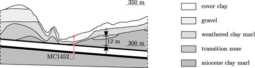
There, the cross-sectional area is around $119\hspace{0.17em}{\mathrm{m}}^2,$ falling into three portions: $53.5\hspace{0.17em}{\mathrm{m}}^2$ are associated with the top heading, $2\times 21\hspace{0.17em}{\mathrm{m}}^2$ are associated with the benches, and $23.7\hspace{0.17em}{\mathrm{m}}^2$ are associated with the invert [55]. The radius of the tunnel shell in the top heading amounts to R = 6.2 m, and its opening angle amounts to $\Delta \phi$ = 167.3°, see Figure 3. The top heading was equipped with three measurement points (MPs), MP1, MP2, and MP3, see Figure 3, where optical reflectors were mounted to the inner surface of the shell, allowing for laser-optical measurements of displacement vectors; and we here consider the corresponding measurements over the first 21 days of the lifetime of the Sieberg tunnel, see Table A2 in Appendix A.

3.2. Measurement data-motivated piecewisely linear evolutions of displacement and force quantities

The measured displacements are not recorded in terms of continuous functions, $\mathbf{u}(t),$ but rather in terms of values recorded at discrete time instants, denoted by t_n, whereby $n=1,\dots ,N_t,$ with N_t as the total number of time instants. All these time instants are measured with respect to $t_0=0.$ In this context, time intervals are denoted by $\Delta t_n=t_n-t_{n-1}.$ More specifically, the records encompass discrete values in a Cartesian base frame, $u_x^{\text{MP}i}(t_n)$ and $u_y^{\text{MP}i}(t_n),$ with i = 1, 2, 3, which can be converted, through the standard vector component transformation rules, into polar values $u_r^{\text{MP}i}(t_n)$ and $u_{\phi }^{\text{MP}i}(t_n),$ with i = 1, 2, 3, see Appendix A. Hence, the relations (26)(26) $$\begin{array}{c}+{\dot{u}}_r^M(\overline{\phi },t)-{\dot{u}}_{\phi ,\mathit{\text{RI}}}^M(t)\hspace{0.17em}\mathrm{\text{sin}}\hspace{0.17em}(\overline{\phi })-{\dot{u}}_{r,\mathit{\text{RI}}}^M(t)\hspace{0.17em}\mathrm{\text{cos}}\hspace{0.17em}(\overline{\phi })+R {\dot{\theta }}_{z,\mathit{\text{RI}}}^M(t)\hspace{0.17em}\mathrm{\text{sin}}\hspace{0.17em}(\overline{\phi })\hfill \\ =+{\mathcal{I}}_{N\to r}(\overline{\phi })[{\int }_0^t\frac{\partial J^{\sigma }}{\partial t}(\xi (t),\eta ({\overline{\sigma }}_{\phi \phi }(t),{\overline{\sigma }}_{\mathit{\text{zz}}}(t)),t-\tau ){\dot{N}}_p(\tau )\mathrm{d}\tau ]\hfill \\ +\sum _{i=1}^4\{{\mathcal{I}}_{i\to r}(\overline{\phi })[{\int }_0^t\frac{\partial J^{\sigma }}{\partial t}(\xi (t),\eta ({\overline{\sigma }}_{\phi \phi }(t),{\overline{\sigma }}_{\mathit{\text{zz}}}(t)),t-\tau ){\dot{G}}_{p,i}(\tau )\mathrm{d}\tau \left]\right\},\hfill \end{array}$$(26) – (28)(28) $$\begin{array}{c}+{\dot{\theta }}_z^M(\overline{\phi },t)-{\dot{\theta }}_{z,\mathit{\text{RI}}}^M(t)\hfill \\ =+{\mathcal{I}}_{N\to z}(\overline{\phi })[{\int }_0^t\frac{\partial J^{\sigma }}{\partial t}(\xi (t),\eta ({\overline{\sigma }}_{\phi \phi }(t),{\overline{\sigma }}_{\mathit{\text{zz}}}(t)),t-\tau ){\dot{N}}_p(\tau )\mathrm{d}\tau ]\hfill \\ +\sum _{i=1}^4\{{\mathcal{I}}_{i\to z}(\overline{\phi })[{\int }_0^t\frac{\partial J^{\sigma }}{\partial t}(\xi (t),\eta ({\overline{\sigma }}_{\phi \phi }(t),{\overline{\sigma }}_{\mathit{\text{zz}}}(t)),t-\tau ){\dot{G}}_{p,i}(\tau )\mathrm{d}\tau \left]\right\}.\hfill \end{array}$$(28) need to be transformed such that displacement and force quantities appear only as values encountered at the aforementioned time instants. For this purpose, we consider piecewisely linear evolution of displacement and force quantities between the aforementioned time instants, and we identify the slope of the evolution between the time instants $t_{n-1},$ and t_n as the rate of the respective quantity at time instant t_n In mathematical terms, the corresponding rates read as (35) $${\dot{u}}_r(t_n)\approx \frac{u_r(t_n)-u_r(t_{n-1})}{\Delta t_n},\hspace{1em}\forall n\in [1,\dots ,N_t],$$(35) (36) $${\dot{u}}_{\phi }(t_n)\approx \frac{u_{\phi }(t_n)-u_{\phi }(t_{n-1})}{\Delta t_n},\hspace{1em}\forall n\in [1,\dots ,N_t],$$(36) (37) $${\dot{\theta }}_z(t_n)\approx \frac{{\theta }_z(t_n)-{\theta }_z(t_{n-1})}{\Delta t_n},\hspace{1em}\forall n\in [1,\dots ,N_t],$$(37) (38) $${\dot{N}}_p(t_n)\approx \frac{N_p(t_n)-N_p(t_{n-1})}{\Delta t_n},\hspace{1em}\forall n\in [1,\dots ,N_t],$$(38) (39) $${\dot{G}}_{p,i}(t_n)\approx \frac{G_{p,i}(t_n)-G_{p,i}(t_{n-1})}{\Delta t_n},\hspace{1em}\forall n\in [1,\dots ,N_t],\text{and}\forall \mathrm{i}\in [1,2,3,4].$$(39)

The correspondingly discretized versions of Eqs. (26)–(28)(28) $$\begin{array}{c}+{\dot{\theta }}_z^M(\overline{\phi },t)-{\dot{\theta }}_{z,\mathit{\text{RI}}}^M(t)\hfill \\ =+{\mathcal{I}}_{N\to z}(\overline{\phi })[{\int }_0^t\frac{\partial J^{\sigma }}{\partial t}(\xi (t),\eta ({\overline{\sigma }}_{\phi \phi }(t),{\overline{\sigma }}_{\mathit{\text{zz}}}(t)),t-\tau ){\dot{N}}_p(\tau )\mathrm{d}\tau ]\hfill \\ +\sum _{i=1}^4\{{\mathcal{I}}_{i\to z}(\overline{\phi })[{\int }_0^t\frac{\partial J^{\sigma }}{\partial t}(\xi (t),\eta ({\overline{\sigma }}_{\phi \phi }(t),{\overline{\sigma }}_{\mathit{\text{zz}}}(t)),t-\tau ){\dot{G}}_{p,i}(\tau )\mathrm{d}\tau \left]\right\}.\hfill \end{array}$$(28) are evaluated N_t times. Each of these versions allows for computing, from ground pressure and impost values known at time instant $t_{n-1},$ the corresponding force quantities associated with time instant t_n. This, however, requires, at all time instants t_n, with $n=1,\dots ,N_t,$ the approximation of convolution integrals which read as (40) $${\mathfrak{C}}_N(t)={\int }_0^t\frac{\partial J^{\sigma }}{\partial t}(\xi (t),\eta ({\overline{\sigma }}_{\phi \phi }(t),{\overline{\sigma }}_{\mathit{\text{zz}}}(t)),t-\tau ){\dot{N}}_p(\tau )\mathrm{d}\tau ,$$(40) and as (41) $${\mathfrak{C}}_G(t)={\int }_0^t\frac{\partial J^{\sigma }}{\partial t}(\xi (t),\eta ({\overline{\sigma }}_{\phi \phi }(t),{\overline{\sigma }}_{\mathit{\text{zz}}}(t)),t-\tau ){\dot{G}}_{p,i}(\tau )\mathrm{d}\tau ,\hspace{1em}\forall i\in [1,2,3,4].$$(41)

This will be tackled next.

3.3. Evaluation and approximation of convolution integrals

Equations (40)(40) $${\mathfrak{C}}_N(t)={\int }_0^t\frac{\partial J^{\sigma }}{\partial t}(\xi (t),\eta ({\overline{\sigma }}_{\phi \phi }(t),{\overline{\sigma }}_{\mathit{\text{zz}}}(t)),t-\tau ){\dot{N}}_p(\tau )\mathrm{d}\tau ,$$(40) and (41)(41) $${\mathfrak{C}}_G(t)={\int }_0^t\frac{\partial J^{\sigma }}{\partial t}(\xi (t),\eta ({\overline{\sigma }}_{\phi \phi }(t),{\overline{\sigma }}_{\mathit{\text{zz}}}(t)),t-\tau ){\dot{G}}_{p,i}(\tau )\mathrm{d}\tau ,\hspace{1em}\forall i\in [1,2,3,4].$$(41) cannot be exactly evaluated at any current time instant t_n, as the corresponding mean stresses are not known yet. Quite contrarily, the latter will be actually determined from this very equations. Hence, when it comes to the additional creep compliance due to high stresses, the mean stresses at time instant t_n will be simply approximated by those already known for time instant $t_{n-1}.$ Correspondingly, the affinity factor can be taken out of the convolution integral. Furthermore, the force rates will be considered constant during time interval $\Delta t_n$ and approximated through Eqs. (38)(38) $${\dot{N}}_p(t_n)\approx \frac{N_p(t_n)-N_p(t_{n-1})}{\Delta t_n},\hspace{1em}\forall n\in [1,\dots ,N_t],$$(38) and (39)(39) $${\dot{G}}_{p,i}(t_n)\approx \frac{G_{p,i}(t_n)-G_{p,i}(t_{n-1})}{\Delta t_n},\hspace{1em}\forall n\in [1,\dots ,N_t],\text{and}\forall \mathrm{i}\in [1,2,3,4].$$(39) , and consistently, the creep function rate according to Eq. (11)(11) $$\begin{array}{ccc}\frac{\partial J^{\sigma }}{\partial t}(\xi (t),\eta (\mathit{\sigma }(t)),t-\tau )& =& +\delta (t-\tau )\left\{\frac{1}{E(\xi (t))}+\frac{\eta (\mathit{\sigma }(t))}{E_c(\xi (t))}{\left[\frac{t-\tau }{t_0^{*}}\right]}^{\beta }\right\}\\ & & +H(t-\tau )\left\{\frac{\eta (\mathit{\sigma }(t))}{E_c(\xi (t))}\frac{\beta }{t_0^{*}}{\left[\frac{t-\tau }{t_0^{*}}\right]}^{\beta -1}\right\}.\end{array}$$(11) will be considered as temporally constant as well. In mathematical terms, all these steps result in (42) $$\begin{array}{l}{\mathfrak{C}}_N(t_n)={\int }_0^{t_n}\frac{\partial J^{\sigma }}{\partial t}(\xi (t),\eta ({\overline{\sigma }}_{\phi \phi }(t),{\overline{\sigma }}_{\mathit{\text{zz}}}(t)),t-\tau ){\dot{N}}_p(\tau )\mathrm{d}\tau \hfill \\ \approx \sum _{m=1}^{N_t}\frac{\eta ({\overline{\sigma }}_{\phi \phi }(t_{n-1}),{\overline{\sigma }}_{\mathit{\text{zz}}}(t_{n-1}))}{E_c(\xi (t_n))}\frac{\beta }{t_0^{*}}{\left(\frac{t_n-t_m}{t_0^{*}}\right)}^{\beta -1}\mathrm{}\mathrm{}\times [N_p(t_m)-N_p(t_{m-1})]\hfill \\ +\frac{N_p(t_n)-N_p(t_{n-1})}{E(\xi (t_n))\Delta t_n},\hspace{1em}\forall n\in [1,\dots ,N_t],\end{array}$$(42) and (43) $$\begin{array}{l}{\mathfrak{C}}_{G,i}(t_n)={\int }_0^{t_n}\frac{\partial J^{\sigma }}{\partial t}(\xi (t),\eta ({\overline{\sigma }}_{\phi \phi }(t),{\overline{\sigma }}_{\mathit{\text{zz}}}(t)),t-\tau ){\dot{G}}_{p,i}(\tau )\mathrm{d}\tau \hfill \\ \approx \sum _{m=1}^{N_t}\frac{\eta ({\overline{\sigma }}_{\phi \phi }(t_{n-1}),{\overline{\sigma }}_{\mathit{\text{zz}}}(t_{n-1}))}{E_c(\xi (t_n))}\frac{\beta }{t_0^{*}}{\left(\frac{t_n-t_m}{t_0^{*}}\right)}^{\beta -1}\mathrm{}\mathrm{}\times [G_{p,j}(t_m)-G_{p,j}(t_{m-1})]\hfill \\ +\frac{G_{p,j}(t_n)-G_{p,j}(t_{n-1})}{E(\xi (t_n))\Delta t_n},\hspace{1em}\forall n\in [1,\dots ,N_t],\text{and}\forall \mathrm{i}\in [1,2,3,4].\hfill \end{array}$$(43)

3.4. Sequential displacement-to-force conversion

Insertion of Eqs. (35)–(39)(39) $${\dot{G}}_{p,i}(t_n)\approx \frac{G_{p,i}(t_n)-G_{p,i}(t_{n-1})}{\Delta t_n},\hspace{1em}\forall n\in [1,\dots ,N_t],\text{and}\forall \mathrm{i}\in [1,2,3,4].$$(39) , as well as of Eqs. (42)–(43)(43) $$\begin{array}{l}{\mathfrak{C}}_{G,i}(t_n)={\int }_0^{t_n}\frac{\partial J^{\sigma }}{\partial t}(\xi (t),\eta ({\overline{\sigma }}_{\phi \phi }(t),{\overline{\sigma }}_{\mathit{\text{zz}}}(t)),t-\tau ){\dot{G}}_{p,i}(\tau )\mathrm{d}\tau \hfill \\ \approx \sum _{m=1}^{N_t}\frac{\eta ({\overline{\sigma }}_{\phi \phi }(t_{n-1}),{\overline{\sigma }}_{\mathit{\text{zz}}}(t_{n-1}))}{E_c(\xi (t_n))}\frac{\beta }{t_0^{*}}{\left(\frac{t_n-t_m}{t_0^{*}}\right)}^{\beta -1}\mathrm{}\mathrm{}\times [G_{p,j}(t_m)-G_{p,j}(t_{m-1})]\hfill \\ +\frac{G_{p,j}(t_n)-G_{p,j}(t_{n-1})}{E(\xi (t_n))\Delta t_n},\hspace{1em}\forall n\in [1,\dots ,N_t],\text{and}\forall \mathrm{i}\in [1,2,3,4].\hfill \end{array}$$(43) together with Eqs. (16)(16) $$\eta =1+2 {\mathcal{U}}^4.$$(16) and (17)(17) $$\begin{array}{lll}\mathcal{U}(r,\phi ,t)& =& +\frac{{\alpha }_{\mathit{\text{DP}}}}{k_{\mathit{\text{DP}}}}[{\sigma }_{\phi \phi }(r,\phi ,t)+{\sigma }_{\mathit{\text{zz}}}(r,\phi ,t)]+\frac{1}{k_{\mathit{\text{DP}}}}\left\{\frac{2}{3}\right[{({\sigma }_{\phi \phi }(r,\phi ,t))}^2\\ & & -{\sigma }_{\phi \phi }(r,\phi ,t){\sigma }_{\mathit{\text{zz}}}(r,\phi ,t)+{({\sigma }_{\mathit{\text{zz}}}(r,\phi ,t))}^2]{\}}^{1/2},\end{array}$$(17) , into the rate Eqs. (26)–(28)(28) $$\begin{array}{c}+{\dot{\theta }}_z^M(\overline{\phi },t)-{\dot{\theta }}_{z,\mathit{\text{RI}}}^M(t)\hfill \\ =+{\mathcal{I}}_{N\to z}(\overline{\phi })[{\int }_0^t\frac{\partial J^{\sigma }}{\partial t}(\xi (t),\eta ({\overline{\sigma }}_{\phi \phi }(t),{\overline{\sigma }}_{\mathit{\text{zz}}}(t)),t-\tau ){\dot{N}}_p(\tau )\mathrm{d}\tau ]\hfill \\ +\sum _{i=1}^4\{{\mathcal{I}}_{i\to z}(\overline{\phi })[{\int }_0^t\frac{\partial J^{\sigma }}{\partial t}(\xi (t),\eta ({\overline{\sigma }}_{\phi \phi }(t),{\overline{\sigma }}_{\mathit{\text{zz}}}(t)),t-\tau ){\dot{G}}_{p,i}(\tau )\mathrm{d}\tau \left]\right\}.\hfill \end{array}$$(28) yields displacement-force relations for each time instant t_n, $n=1,\dots ,N_t,$ given in the following format. (44) $$\begin{array}{l}\hfill \\ +\frac{u_r^M(\overline{\phi },t_n)-u_r^M(\overline{\phi },t_{n-1})}{\Delta t_n}-\frac{u_{r,\mathit{\text{RI}}}^M(t_n)-u_{r,\mathit{\text{RI}}}^M(t_{n-1})}{\Delta t_n}[\mathrm{\text{cos}}\hspace{0.17em}(\overline{\phi })]\hfill \\ -\frac{u_{\phi ,\mathit{\text{RI}}}^M(t_n)-u_{\phi ,\mathit{\text{RI}}}^M(t_{n-1})}{\Delta t_n}[\mathrm{\text{sin}}\hspace{0.17em}(\overline{\phi })]+\frac{R {\theta }_{z,\mathit{\text{RI}}}^M(t_n)-R {\theta }_{z,\mathit{\text{RI}}}^M(t_{n-1})}{\Delta t_n}[\mathrm{\text{sin}}\hspace{0.17em}(\overline{\phi })]\hfill \\ \begin{array}{cc}=\hfill & \mathrm{}\mathrm{}+{\mathcal{I}}_{N\to r}(\overline{\phi })\{\eta ({\overline{\sigma }}_{\phi \phi }(t_{n-1}),{\overline{\sigma }}_{\mathit{\text{zz}}}(t_{n-1}))\sum _{m=1}^{N_t}\frac{\beta /t_0^{*}}{E_c(\xi (t_n))}{\left(\frac{t_n-t_m}{t_0^{*}}\right)}^{\beta -1}\hfill \\ \hfill & \times [N_p(t_m)-N_p(t_{m-1})]+\frac{N_p(t_n)-N_p(t_{n-1})}{E(\xi (t_n))\Delta t_n}\}\hfill \\ \hfill & \mathrm{}\mathrm{}+\sum _{j=1}^4\{{\mathcal{I}}_{j\to r}(\overline{\phi })\{\eta ({\overline{\sigma }}_{\phi \phi }(t_{n-1}),{\overline{\sigma }}_{\mathit{\text{zz}}}(t_{n-1}))\sum _{m=1}^{N_t}\frac{\beta /t_0^{*}}{E_c(\xi (t_n))}{\left(\frac{t_n-t_m}{t_0^{*}}\right)}^{\beta -1}\hfill \\ \hfill & \times [G_{p,j}(t_m)-G_{p,j}(t_{m-1})]+\frac{G_{p,j}(t_n)-G_{p,j}(t_{n-1})}{E(\xi (t_n))\Delta t_n}\left\}\right\},\hfill \end{array}\hfill \end{array}$$(44) (45) $$\begin{array}{c}+\frac{u_{\phi }^M(\overline{\phi },t_n)-u_{\phi }^M(\overline{\phi },t_{n-1})}{\Delta t_n}+\frac{u_{r,\mathit{\text{RI}}}^M(t_n)-u_{r,\mathit{\text{RI}}}^M(t_{n-1})}{\Delta t_n}[\mathrm{\text{sin}}\hspace{0.17em}(\overline{\phi })]\hfill \\ -\frac{u_{\phi ,\mathit{\text{RI}}}^M(t_n)-u_{\phi ,\mathit{\text{RI}}}^M(t_{n-1})}{\Delta t_n}[\mathrm{\text{cos}}\hspace{0.17em}(\overline{\phi })]+\frac{R {\theta }_{z,\mathit{\text{RI}}}^M(t_n)-R {\theta }_{z,\mathit{\text{RI}}}^M(t_{n-1})}{\Delta t_n}[\mathrm{\text{cos}}\hspace{0.17em}(\overline{\phi })-1]\hfill \\ \begin{array}{cc}=\hfill & \mathrm{}\mathrm{}+{\mathcal{I}}_{N\to \phi }(\overline{\phi })\{\eta ({\overline{\sigma }}_{\phi \phi }(t_{n-1}),{\overline{\sigma }}_{\mathit{\text{zz}}}(t_{n-1}))\sum _{m=1}^{N_t}\frac{\beta /t_0^{*}}{E_c(\xi (t_n))}{\left(\frac{t_n-t_m}{t_0^{*}}\right)}^{\beta -1}\hfill \\ \hfill & \times [N_p(t_m)-N_p(t_{m-1})]+\frac{N_p(t_n)-N_p(t_{n-1})}{E(\xi (t_n))\Delta t_n}\}\hfill \\ \hfill & \mathrm{}\mathrm{}+\sum _{j=1}^4\{{\mathcal{I}}_{j\to \phi }(\overline{\phi })\{\eta ({\overline{\sigma }}_{\phi \phi }(t_{n-1}),{\overline{\sigma }}_{\mathit{\text{zz}}}(t_{n-1}))\sum _{m=1}^{N_t}\frac{\beta /t_0^{*}}{E_c(\xi (t_n))}{\left(\frac{t_n-t_m}{t_0^{*}}\right)}^{\beta -1}\hfill \\ \hfill & \times [G_{p,j}(t_m)-G_{p,j}(t_{m-1})]+\frac{G_{p,j}(t_n)-G_{p,j}(t_{n-1})}{E(\xi (t_n))\Delta t_n}\left\}\right\},\hfill \end{array}\hfill \end{array}$$(45) (46) $$\begin{array}{c}+\frac{{\theta }_z^M(\overline{\phi },t_n)-{\theta }_z^M(\overline{\phi },t_{n-1})}{\Delta t_n}-\frac{{\theta }_{z,\mathit{\text{RI}}}^M(t_n)-{\theta }_{z,\mathit{\text{RI}}}^M(t_{n-1})}{\Delta t_n}\hfill \\ \begin{array}{cc}=\hfill & \mathrm{}\mathrm{}+{\mathcal{I}}_{N\to z}(\overline{\phi })\{\eta ({\overline{\sigma }}_{\phi \phi }(t_{n-1}),{\overline{\sigma }}_{\mathit{\text{zz}}}(t_{n-1}))\sum _{m=1}^{N_t}\frac{\beta /t_0^{*}}{E_c(\xi (t_n))}{\left(\frac{t_n-t_m}{t_0^{*}}\right)}^{\beta -1}\hfill \\ \hfill & \times [N_p(t_m)-N_p(t_{m-1})]+\frac{N_p(t_n)-N_p(t_{n-1})}{E(\xi (t_n))\Delta t_n}\}\hfill \\ \hfill & \mathrm{}\mathrm{}+\sum _{j=1}^4\{{\mathcal{I}}_{j\to z}(\overline{\phi })\{\eta ({\overline{\sigma }}_{\phi \phi }(t_{n-1}),{\overline{\sigma }}_{\mathit{\text{zz}}}(t_{n-1}))\sum _{m=1}^{N_t}\frac{\beta /t_0^{*}}{E_c(\xi (t_n))}{\left(\frac{t_n-t_m}{t_0^{*}}\right)}^{\beta -1}\hfill \\ \hfill & \times [G_{p,j}(t_m)-G_{p,j}(t_{m-1})]+\frac{G_{p,j}(t_n)-G_{p,j}(t_{n-1})}{E(\xi (t_n))\Delta t_n}\left\}\right\}.\hfill \end{array}\hfill \end{array}$$(46)

From Eqs. (44)–(46)(46) $$\begin{array}{c}+\frac{{\theta }_z^M(\overline{\phi },t_n)-{\theta }_z^M(\overline{\phi },t_{n-1})}{\Delta t_n}-\frac{{\theta }_{z,\mathit{\text{RI}}}^M(t_n)-{\theta }_{z,\mathit{\text{RI}}}^M(t_{n-1})}{\Delta t_n}\hfill \\ \begin{array}{cc}=\hfill & \mathrm{}\mathrm{}+{\mathcal{I}}_{N\to z}(\overline{\phi })\{\eta ({\overline{\sigma }}_{\phi \phi }(t_{n-1}),{\overline{\sigma }}_{\mathit{\text{zz}}}(t_{n-1}))\sum _{m=1}^{N_t}\frac{\beta /t_0^{*}}{E_c(\xi (t_n))}{\left(\frac{t_n-t_m}{t_0^{*}}\right)}^{\beta -1}\hfill \\ \hfill & \times [N_p(t_m)-N_p(t_{m-1})]+\frac{N_p(t_n)-N_p(t_{n-1})}{E(\xi (t_n))\Delta t_n}\}\hfill \\ \hfill & \mathrm{}\mathrm{}+\sum _{j=1}^4\{{\mathcal{I}}_{j\to z}(\overline{\phi })\{\eta ({\overline{\sigma }}_{\phi \phi }(t_{n-1}),{\overline{\sigma }}_{\mathit{\text{zz}}}(t_{n-1}))\sum _{m=1}^{N_t}\frac{\beta /t_0^{*}}{E_c(\xi (t_n))}{\left(\frac{t_n-t_m}{t_0^{*}}\right)}^{\beta -1}\hfill \\ \hfill & \times [G_{p,j}(t_m)-G_{p,j}(t_{m-1})]+\frac{G_{p,j}(t_n)-G_{p,j}(t_{n-1})}{E(\xi (t_n))\Delta t_n}\left\}\right\}.\hfill \end{array}\hfill \end{array}$$(46) , displacement data recorded at the three measurement points MP1, MP2, and MP3, indicated in Figure 3, can be translated, at each time instant t_n, $n=1,2,\dots ,N_t,$ into ground pressure values $G_{p,i}(t_n),i=1,2,3,4,$ and impost force values $N_p(t_n).$ In more detail, seven unknowns, namely $G_{p,1}(t_n),G_{p,2}(t_n),G_{p,3}(t_n),G_{p,4}(t_n),N_p(t_n),{\theta }_{z,\mathit{\text{RI}}}^M(t_n)={\theta }_z^M(\overline{\phi }\mathrm{}=\mathrm{}0),$ and ${\theta }_{z,\mathit{\text{LI}}}^M(t_n)={\theta }_z^M(\overline{\phi }\mathrm{}=\mathrm{}\Delta \phi ),$ need to be determined from a linear system of seven equations. The latter are obtained as follows:

• Two equations result from specification of the natural boundary condition, Eq. (32)(32) $$\frac{1}{R}\frac{\mathrm{d}{m}_z}{\mathrm{d}\phi }=0.$$(32) , for the left and right impost of the arch-like tunnel cross section, $\overline{\phi }=0$ and $\overline{\phi }=\Delta \phi ,$ as well as for Eq. (31)(31) $$m_z(\overline{\phi })=+R N_p {\mathcal{I}}_{N\to m}(\overline{\phi })+\sum _{i=1}^4[R^2 G_{p,i} {\mathcal{I}}_{i\to n}(\overline{\phi })],$$(31) .

• Two equations result from specification of the discretized format of the radial displacements according to Eq. (44)(44) $$\begin{array}{l}\hfill \\ +\frac{u_r^M(\overline{\phi },t_n)-u_r^M(\overline{\phi },t_{n-1})}{\Delta t_n}-\frac{u_{r,\mathit{\text{RI}}}^M(t_n)-u_{r,\mathit{\text{RI}}}^M(t_{n-1})}{\Delta t_n}[\mathrm{\text{cos}}\hspace{0.17em}(\overline{\phi })]\hfill \\ -\frac{u_{\phi ,\mathit{\text{RI}}}^M(t_n)-u_{\phi ,\mathit{\text{RI}}}^M(t_{n-1})}{\Delta t_n}[\mathrm{\text{sin}}\hspace{0.17em}(\overline{\phi })]+\frac{R {\theta }_{z,\mathit{\text{RI}}}^M(t_n)-R {\theta }_{z,\mathit{\text{RI}}}^M(t_{n-1})}{\Delta t_n}[\mathrm{\text{sin}}\hspace{0.17em}(\overline{\phi })]\hfill \\ \begin{array}{cc}=\hfill & \mathrm{}\mathrm{}+{\mathcal{I}}_{N\to r}(\overline{\phi })\{\eta ({\overline{\sigma }}_{\phi \phi }(t_{n-1}),{\overline{\sigma }}_{\mathit{\text{zz}}}(t_{n-1}))\sum _{m=1}^{N_t}\frac{\beta /t_0^{*}}{E_c(\xi (t_n))}{\left(\frac{t_n-t_m}{t_0^{*}}\right)}^{\beta -1}\hfill \\ \hfill & \times [N_p(t_m)-N_p(t_{m-1})]+\frac{N_p(t_n)-N_p(t_{n-1})}{E(\xi (t_n))\Delta t_n}\}\hfill \\ \hfill & \mathrm{}\mathrm{}+\sum _{j=1}^4\{{\mathcal{I}}_{j\to r}(\overline{\phi })\{\eta ({\overline{\sigma }}_{\phi \phi }(t_{n-1}),{\overline{\sigma }}_{\mathit{\text{zz}}}(t_{n-1}))\sum _{m=1}^{N_t}\frac{\beta /t_0^{*}}{E_c(\xi (t_n))}{\left(\frac{t_n-t_m}{t_0^{*}}\right)}^{\beta -1}\hfill \\ \hfill & \times [G_{p,j}(t_m)-G_{p,j}(t_{m-1})]+\frac{G_{p,j}(t_n)-G_{p,j}(t_{n-1})}{E(\xi (t_n))\Delta t_n}\left\}\right\},\hfill \end{array}\hfill \end{array}$$(44) for $u_r^M(\overline{\phi }\mathrm{}=\mathrm{}\Delta \phi /2,t_n)=u_r^{\text{MP}1}(t_n)$ and $u_r^M(\overline{\phi }\mathrm{}=\mathrm{}\Delta \phi ,t_n)=u_r^{\text{MP}2}(t_n),$ and also for $u_{r,\mathit{\text{RI}}}^M=u_r^{\text{MP}3}$ and $u_{\phi ,\mathit{\text{RI}}}^M=u_{\phi }^{\text{MP}3}.$

• Two equations result from specification of the discretized format of the tangential displacements according to Eq. (45)(45) $$\begin{array}{c}+\frac{u_{\phi }^M(\overline{\phi },t_n)-u_{\phi }^M(\overline{\phi },t_{n-1})}{\Delta t_n}+\frac{u_{r,\mathit{\text{RI}}}^M(t_n)-u_{r,\mathit{\text{RI}}}^M(t_{n-1})}{\Delta t_n}[\mathrm{\text{sin}}\hspace{0.17em}(\overline{\phi })]\hfill \\ -\frac{u_{\phi ,\mathit{\text{RI}}}^M(t_n)-u_{\phi ,\mathit{\text{RI}}}^M(t_{n-1})}{\Delta t_n}[\mathrm{\text{cos}}\hspace{0.17em}(\overline{\phi })]+\frac{R {\theta }_{z,\mathit{\text{RI}}}^M(t_n)-R {\theta }_{z,\mathit{\text{RI}}}^M(t_{n-1})}{\Delta t_n}[\mathrm{\text{cos}}\hspace{0.17em}(\overline{\phi })-1]\hfill \\ \begin{array}{cc}=\hfill & \mathrm{}\mathrm{}+{\mathcal{I}}_{N\to \phi }(\overline{\phi })\{\eta ({\overline{\sigma }}_{\phi \phi }(t_{n-1}),{\overline{\sigma }}_{\mathit{\text{zz}}}(t_{n-1}))\sum _{m=1}^{N_t}\frac{\beta /t_0^{*}}{E_c(\xi (t_n))}{\left(\frac{t_n-t_m}{t_0^{*}}\right)}^{\beta -1}\hfill \\ \hfill & \times [N_p(t_m)-N_p(t_{m-1})]+\frac{N_p(t_n)-N_p(t_{n-1})}{E(\xi (t_n))\Delta t_n}\}\hfill \\ \hfill & \mathrm{}\mathrm{}+\sum _{j=1}^4\{{\mathcal{I}}_{j\to \phi }(\overline{\phi })\{\eta ({\overline{\sigma }}_{\phi \phi }(t_{n-1}),{\overline{\sigma }}_{\mathit{\text{zz}}}(t_{n-1}))\sum _{m=1}^{N_t}\frac{\beta /t_0^{*}}{E_c(\xi (t_n))}{\left(\frac{t_n-t_m}{t_0^{*}}\right)}^{\beta -1}\hfill \\ \hfill & \times [G_{p,j}(t_m)-G_{p,j}(t_{m-1})]+\frac{G_{p,j}(t_n)-G_{p,j}(t_{n-1})}{E(\xi (t_n))\Delta t_n}\left\}\right\},\hfill \end{array}\hfill \end{array}$$(45) for $u_{\phi }^M(\overline{\phi }\mathrm{}=\mathrm{}\Delta \phi /2,t_n)=u_{\phi }^{\text{MP}1}(t_n)$ and $u_{\phi }^M(\overline{\phi }\mathrm{}=\mathrm{}\Delta \phi ,t_n)=u_{\phi }^{\text{MP}2}(t_n),$ and also for $u_{r,\mathit{\text{RI}}}^M=u_r^{\text{MP}3}$ and $u_{\phi ,\mathit{\text{RI}}}^M=u_{\phi }^{\text{MP}3}.$

• One equation results from specification of the discretized format of the rotation angle according to Eq. (46)(46) $$\begin{array}{c}+\frac{{\theta }_z^M(\overline{\phi },t_n)-{\theta }_z^M(\overline{\phi },t_{n-1})}{\Delta t_n}-\frac{{\theta }_{z,\mathit{\text{RI}}}^M(t_n)-{\theta }_{z,\mathit{\text{RI}}}^M(t_{n-1})}{\Delta t_n}\hfill \\ \begin{array}{cc}=\hfill & \mathrm{}\mathrm{}+{\mathcal{I}}_{N\to z}(\overline{\phi })\{\eta ({\overline{\sigma }}_{\phi \phi }(t_{n-1}),{\overline{\sigma }}_{\mathit{\text{zz}}}(t_{n-1}))\sum _{m=1}^{N_t}\frac{\beta /t_0^{*}}{E_c(\xi (t_n))}{\left(\frac{t_n-t_m}{t_0^{*}}\right)}^{\beta -1}\hfill \\ \hfill & \times [N_p(t_m)-N_p(t_{m-1})]+\frac{N_p(t_n)-N_p(t_{n-1})}{E(\xi (t_n))\Delta t_n}\}\hfill \\ \hfill & \mathrm{}\mathrm{}+\sum _{j=1}^4\{{\mathcal{I}}_{j\to z}(\overline{\phi })\{\eta ({\overline{\sigma }}_{\phi \phi }(t_{n-1}),{\overline{\sigma }}_{\mathit{\text{zz}}}(t_{n-1}))\sum _{m=1}^{N_t}\frac{\beta /t_0^{*}}{E_c(\xi (t_n))}{\left(\frac{t_n-t_m}{t_0^{*}}\right)}^{\beta -1}\hfill \\ \hfill & \times [G_{p,j}(t_m)-G_{p,j}(t_{m-1})]+\frac{G_{p,j}(t_n)-G_{p,j}(t_{n-1})}{E(\xi (t_n))\Delta t_n}\left\}\right\}.\hfill \end{array}\hfill \end{array}$$(46) for ${\theta }_z^M(\overline{\phi }\mathrm{}=\mathrm{}\Delta \phi ,t_n)={\theta }_{z,\mathit{\text{LI}}}^M(t_n).$

This system is solved at every time instant t_n. In addition, degenerated forms of Eqs. (44)–(46)(46) $$\begin{array}{c}+\frac{{\theta }_z^M(\overline{\phi },t_n)-{\theta }_z^M(\overline{\phi },t_{n-1})}{\Delta t_n}-\frac{{\theta }_{z,\mathit{\text{RI}}}^M(t_n)-{\theta }_{z,\mathit{\text{RI}}}^M(t_{n-1})}{\Delta t_n}\hfill \\ \begin{array}{cc}=\hfill & \mathrm{}\mathrm{}+{\mathcal{I}}_{N\to z}(\overline{\phi })\{\eta ({\overline{\sigma }}_{\phi \phi }(t_{n-1}),{\overline{\sigma }}_{\mathit{\text{zz}}}(t_{n-1}))\sum _{m=1}^{N_t}\frac{\beta /t_0^{*}}{E_c(\xi (t_n))}{\left(\frac{t_n-t_m}{t_0^{*}}\right)}^{\beta -1}\hfill \\ \hfill & \times [N_p(t_m)-N_p(t_{m-1})]+\frac{N_p(t_n)-N_p(t_{n-1})}{E(\xi (t_n))\Delta t_n}\}\hfill \\ \hfill & \mathrm{}\mathrm{}+\sum _{j=1}^4\{{\mathcal{I}}_{j\to z}(\overline{\phi })\{\eta ({\overline{\sigma }}_{\phi \phi }(t_{n-1}),{\overline{\sigma }}_{\mathit{\text{zz}}}(t_{n-1}))\sum _{m=1}^{N_t}\frac{\beta /t_0^{*}}{E_c(\xi (t_n))}{\left(\frac{t_n-t_m}{t_0^{*}}\right)}^{\beta -1}\hfill \\ \hfill & \times [G_{p,j}(t_m)-G_{p,j}(t_{m-1})]+\frac{G_{p,j}(t_n)-G_{p,j}(t_{n-1})}{E(\xi (t_n))\Delta t_n}\left\}\right\}.\hfill \end{array}\hfill \end{array}$$(46) , arising from the choices η = 1, and η = 0, respectively, are converted into simplified systems of equations. The latter give access to shells exhibiting linear aging viscoelastic and aging elastic behavior.

4. Ground pressure, force, and displacement developments in MC1452 of Sieberg tunnel

The following results were obtained for a typical shotcrete mixture with cement type CEM II/A-S 42.5 R, and strength class SpC 20/25, see Table 1, by solving the linear system of seven equations arising from Eqs. (44)–(46)(46) $$\begin{array}{c}+\frac{{\theta }_z^M(\overline{\phi },t_n)-{\theta }_z^M(\overline{\phi },t_{n-1})}{\Delta t_n}-\frac{{\theta }_{z,\mathit{\text{RI}}}^M(t_n)-{\theta }_{z,\mathit{\text{RI}}}^M(t_{n-1})}{\Delta t_n}\hfill \\ \begin{array}{cc}=\hfill & \mathrm{}\mathrm{}+{\mathcal{I}}_{N\to z}(\overline{\phi })\{\eta ({\overline{\sigma }}_{\phi \phi }(t_{n-1}),{\overline{\sigma }}_{\mathit{\text{zz}}}(t_{n-1}))\sum _{m=1}^{N_t}\frac{\beta /t_0^{*}}{E_c(\xi (t_n))}{\left(\frac{t_n-t_m}{t_0^{*}}\right)}^{\beta -1}\hfill \\ \hfill & \times [N_p(t_m)-N_p(t_{m-1})]+\frac{N_p(t_n)-N_p(t_{n-1})}{E(\xi (t_n))\Delta t_n}\}\hfill \\ \hfill & \mathrm{}\mathrm{}+\sum _{j=1}^4\{{\mathcal{I}}_{j\to z}(\overline{\phi })\{\eta ({\overline{\sigma }}_{\phi \phi }(t_{n-1}),{\overline{\sigma }}_{\mathit{\text{zz}}}(t_{n-1}))\sum _{m=1}^{N_t}\frac{\beta /t_0^{*}}{E_c(\xi (t_n))}{\left(\frac{t_n-t_m}{t_0^{*}}\right)}^{\beta -1}\hfill \\ \hfill & \times [G_{p,j}(t_m)-G_{p,j}(t_{m-1})]+\frac{G_{p,j}(t_n)-G_{p,j}(t_{n-1})}{E(\xi (t_n))\Delta t_n}\left\}\right\}.\hfill \end{array}\hfill \end{array}$$(46) , as described just below these equations.

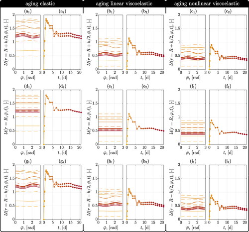
The resulting spatial distributions of displacements and generator rotations are virtually independent of the chosen material model, as can be seen by comparing Figure 5(a₁), (a₂), (d₁), (d₂), (g₁), (g₂) with Figure 5(b₁), (b₂), (e₁), (e₂), (h₁), (h₂), and Figure 5(c₁), (c₂), (f₁), (f₂), (i₁), (i₂).

Figure 5. Distribution of radial and circumferential displacements at shell midsurfaces (a-f), and of generator rotations (g-i) along the circumference of the top heading (index 1) of the Sieberg tunnel at measurement cross section MC1452, and the temporal evolution of maximum and minimum values (index 2) for the time points according to Table A2; determined by hybrid analyses based on aging elasticity (a,d,g), on aging viscoelasticity (b,e,h), on aging nonlinear viscoelasticity (c,f,i), respectively.

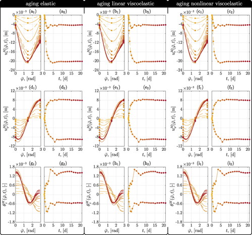
As a rule, the largest absolute values of radial displacements are encountered at the crown of the tunnel, and the largest absolute values of circumferential displacements are encountered at the imposts, with the radial displacements reflecting inward movements and the circumferential displacements reflecting settlements of the midsurface of the investigated tunnel shell. These inward movements and settlements develop during the first five days of the lifetime of the tunnel, and after some subsequent fluctuations, they stabilize after some 10 days, see Figure 5. The inward movements are consistent with a negative (clockwise) generator rotation at the left impost (with $\overline{\phi }=\Delta \phi$) and a positive (counterclockwise) generator rotation at the right impost (with $\overline{\phi }=0$). Over time, the right imposed-related positive rotation is enhanced, while the left imposed-related negative rotation diminishes, which is consistent with the left impost showing larger radial inward movements than the right impost, see Figure 6.

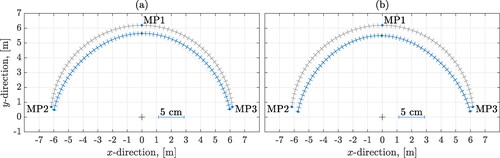
Figure 6. Midsurface displacement distribution with corresponding shell generator lines of length $h=0.30 \mathrm{m}$ at $t=1.264 \mathrm{d}$ (a), and at $t=21 \mathrm{d},$ of the Sieberg tunnel at the measurement cross-section MC1452 (magnification factor of the displacements: 35); determined by hybrid analysis based on aging nonlinear viscoelasticity.

Insertion of the solutions for the variables $G_{p,1},G_{p,2},G_{p,3},G_{p,4},$ and N_p into the external-to-internal force relations (30)(30) $$n_{\phi }(\overline{\phi })=+N_p {\mathcal{I}}_{N\to n}(\overline{\phi })-\sum _{i=1}^4[R G_{p,i} {\mathcal{I}}_{i\to n}(\overline{\phi })],$$(30) and (31)(31) $$m_z(\overline{\phi })=+R N_p {\mathcal{I}}_{N\to m}(\overline{\phi })+\sum _{i=1}^4[R^2 G_{p,i} {\mathcal{I}}_{i\to n}(\overline{\phi })],$$(31) , provides spatial distributions of axial normal forces and of bending moments, see Figure 7(a₁), (b₁), (c₁), (d₁), (e₁), (f₁), while the use of ground pressure value solutions in Eq. (24)(24) $$\begin{array}{lll}{G}_p(\overline{\phi })& =& +A_1(\overline{\phi })\hspace{0.17em}{G}_{p,1}+A_2(\overline{\phi })\hspace{0.17em}{G}_{p,2}+A_3(\overline{\phi })\hspace{0.17em}{G}_{p,3}+A_4(\overline{\phi })\hspace{0.17em}{G}_{p,4},\end{array}$$(24) yields ground pressure distributions, see Figure 7(g₁), (h₁), (i₁): In terms of magnitude of the involved physical quantities, all these distributions are heavily dependent on the chosen material model for shotcrete, with the magnitudes of ground pressure and normal force being reduced by a factor of about three when switching from an aging elasticity model to an aging viscoelastic formulation for highly stressed shotcrete; with the aging version of linear viscoelasticity delivering results lying right between the aforementioned ones. The situation is somewhat different for the bending moments, which are, by comparison, fairly independent of the chosen material model for shotcrete, see Figure 7(d)–(f). As a rule, these bending moments vanish at the imposts, in accordance with the used structural model not permitting moment transmission from the tunnel shell to the surrounding ground. They also vanish at the tunnel crown, but they exhibit remarkable non-zero values in the lateral portions of the tunnel arch. The latter values are negative at the right-hand side of the tunnel arch, which, according to Eq. (21)(21) $$m_z(\phi )=\underset{R-h/2}{\overset{R+h/2}{\int }}{\sigma }_{\phi \phi }(r,\phi )\times (r-R)\mathrm{d}r.$$(21) , comes with bending moment-induced tensile normal stresses at the inner shell surface, and the opposite is true for the left-hand side of tunnel arch, with positive bending moment values and associated tensile normal stresses at the outer shell surface. When compared to the bending moments, the axial normal forces are virtually independent of the spatial position, see Figure 7(a₁), (b₁), (c₁), which is consistent with a virtually uniform ground pressure, see Figure 7(g₁), (h₁), (i₁). They are the main loading factor of the tunnel shell, as seen by virtually constant utilization degree distributions along the midsurface of the tunnel shell, see Figure 8(d₁), (e₁), (f₁). Somewhat differently, the utilization degrees at the inner and outer shell surfaces exhibit an azimuth-dependent fluctuation, see Figure 8(a₁), (b₁), (c₁), (g₁), (h₁), (i₁). These fluctuations are a consequence of the bending moment distributions discussed further above; the latter result from fluctuations in the ground pressure, being larger in the right portion than in the left portion of the tunnel arch, but of such a small magnitude, that they are not discernible in Figure 7(g–i). Conclusively, it turns out that only the consideration of aging nonlinear viscoelastic material behavior provides access to realistic values for the degree of utilization, being lower than one, see Figure 8. Simpler material models would indicate local material failure, which was not observed in situ.

Figure 7. Distribution of circumferential normal forces (a-c), bending moments (d-f), and of ground pressure (g-i) along the circumference of the top heading (index 1) of the Sieberg tunnel at measurement cross section MC1452, and the temporal evolution of maximum and minimum values (index 2) for the time points according to Table A2; determined by hybrid analyses based on aging elasticity (a,d,g), on aging viscoelasticity (b,e,h), on aging nonlinear viscoelasticity (c,f,i), respectively.

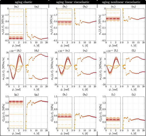
Figure 8. Distribution of degree of utilization for $r=R+h/2$ (a-c), for r = R (d-f), and for $r=R-h/2$ (g-i), along the circumference of the top heading (index 1) of the Sieberg tunnel at measurement cross section MC1452, and the temporal evolution of maximum and minimum values (index 2) for the time points according to Table A2; determined by hybrid analyses based on aging elasticity (a,d,g), on aging viscoelasticity (b,e,h), on aging nonlinear viscoelasticity (c,f,i), respectively.

5. Conclusions

Aging viscoelasticity for highly stressed shotcrete appears as necessary ingredient for the realistic assessment of the forces acting on and within a tunnel shell constructed according to the New Austrian Tunneling Method, with corresponding displacement monitoring data feeding an analytical mechanic model. This is consistent with recent results concerning mechanized tunneling with precast tunnel segments being monitored by vibrating wires, where the use of a viscoelastic, rather than a simple elastic, material model for the used concrete was also key to realistic stress and utilization degree assessment [56]. The combination of Boltzmann’s superposition principle with power-law creep functions, as used here, may also be reformulated in terms of fractional derivatives of the Caputo form [57] – this embeds the present contribution into a wide field of creep applications, comprising not only concrete, but also polymers [58] and semiconductors [59]. Finally, the consideration of aging is key to realistic mechanics modeling for the NATM: Mathematically, this can be met by a constitutive formulation which is exclusively built on stress and strain rates, rather than the current total quantities of stress and strain, as they appear in the traditional format of Hooke’s law. In this context, the overall emerging picture is one where specific forms of stress-rate-strain-rate laws may be integrated so as to deliver total stress-strain laws with clearly limited validity, rather than one where rate laws would result from temporal derivatives of total stress-strain laws. This is consistent with the steadily growing importance of rate-based material modeling ever since Truesdell’s inception of hypoelasticity [35]. In this context, our expression (2)(2) $$\begin{array}{ccc}\mathit{d}(t)& =& {\int }_{-\infty }^t{\mathit{J}}_d(\xi (t),t-\tau ):\dot{\mathit{\sigma }}(\tau )\mathrm{d}\tau ,\end{array}$$(2) can be seen as yet another way of generalizing and broadening more traditional elastic and viscoelastic modeling concepts, in addition to that resting on Gibbs’ thermodynamic potential [38].

Nomenclature
$A_i$	=	cubic shape functions (with $i=1,2,3,4$)
$\mathit{d}$	=	Eulerian strain rate tensor
${\mathbf{e}}_r,{\mathbf{e}}_{\phi },{\mathbf{e}}_z$	=	unit base vectors of (cylindrical) coordinate system, moving along an arc
${\mathbf{e}}_x,{\mathbf{e}}_y,{\mathbf{e}}_z$	=	unit base vectors of Cartesian coordinate system, fixed in space
$E$	=	elastic modulus (Young’s modulus) of shotcrete
$E_{28\mathrm{d}}$	=	28-day value of E
$E_c$	=	creep modulus of shotcrete
$E_{c,28\mathrm{d}}$	=	28-day value of Ec
$f_b$	=	biaxial compressive strength of shotcrete
$f_c$	=	uniaxial compressive strength of shotcrete
$f_c^{*}$	=	reference strength level
$f_{c,28\mathrm{d}}$	=	28-day value of fc
$G_p$	=	ground pressure
$G_{p,i}$	=	ground pressure at position i (with $i=1,2,3,4$)
$h$	=	thickness of tunnel shell segment
$\mathit{J}$	=	4th-order creep function tensor
${\mathit{J}}_d$	=	4th-order creep rate function tensor
${\mathit{J}}^{\sigma }$	=	4th-order creep function tensor associated with highly stressed material
$J$	=	creep function
$k_{\mathit{\text{DP}}}$	=	strength-like quantity in Drucker–Prager failure criterion
m	=	index numbering time steps
$m_z$	=	bending moment around an axis in ${\mathbf{e}}_z$-dircetion and positioned on the midsurface of the tunnel shell segment (per length measured in tunnel driving direction ${\mathit{e}}_z$)
$N_p$	=	impost force (per length measured in tunnel driving direction ${\mathit{e}}_z$)
$N_{p,\mathit{\text{LI}}},N_{p,\mathit{\text{RI}}}$	=	forces at the left and the right impost of the arch-like tunnel cross section, respectively
$N_t$	=	number of time steps
n	=	index numbering time steps
$\mathbf{n}$	=	outward normal onto a surface element
$n_{\phi }$	=	circumferential normal force (per length measured in tunnel driving direction ${\mathit{e}}_z$)
$r$	=	radial coordinate
$R$	=	radius of the undeformed midsurface of a tunnel shell segment
$s_E$	=	dimensionless parameter quantifying strength and Young’s modulus evolution
$s_{E_c}$	=	dimensionless parameter quantifying creep modulus evolution
$t$	=	time variable associated with recording of strain or displacement values
$t_0^{*}$	=	reference time
${\mathcal{T}}_{\mathit{\text{cr}}}$	=	characteristic creep time
${\mathcal{T}}_{\mathit{\text{hyd}}}$	=	characteristic hydration time
$T_r$	=	radial component of the traction vectors acting onto the outer surface of the tunnel shell
$T_{\phi }$	=	circumferential component of the traction vectors acting onto the imposts of the arch-like tunnel cross section
$u_r^M,u_{\phi }^M$	=	radial and circumferential displacements at the midsurface of the cylindrical tunnel shell segments
$u_r^{\text{MP}i},u_{\phi }^{\text{MP}i}$	=	polar displacements recorded at measurement point i (with i = 1, 2, 3)
$u_x^{\text{MP}i},u_y^{\text{MP}i}$	=	Cartesian displacements recorded at measurement point i (with i = 1, 2, 3)
$u_{r,\mathit{\text{RI}}}^M,u_{\phi ,\mathit{\text{RI}}}^M$	=	radial and circumferential displacements of the midsurface at the right impost of the arch-like tunnel cross section
z	=	axial coordinate, associated with tunnel driving direction
$\alpha$	=	dimensionless parameter related to the shotcrete aggregates
${\alpha }_{\mathit{\text{DP}}}$	=	dimensionless parameter of Drucker–Prager failure criterion
$\beta$	=	creep-related power-law exponent
$\Delta \phi$	=	central angle of circular tunnel shell arc
$\Delta t$	=	time increment
$\mathit{\epsilon }$	=	linearized strain tensor
${\epsilon }_{\mathit{\text{ii}}}$	=	normal strain component associated with direction ${\mathbf{e}}_i$ (with $i=r,\phi ,z$)
$\eta$	=	affine creep magnification factor
${\theta }_z^M$	=	rotational angle of the shell generator line, around an axis oriented in ${\mathbf{e}}_z$-direction and positioned on the midsurface of the tunnel shell segment
${\theta }_{z,\mathit{\text{LI}}}^M,{\theta }_{z,\mathit{\text{RI}}}^M$	=	rotational angle of the shell generator line, around an axis oriented in ${\mathbf{e}}_z$-direction and positioned on the midsurface at the left and the right impost of the arch-like tunnel cross section, respectively
$\kappa$	=	ratio of biaxial to uniaxial compressive strength of shotcrete
$\nu$	=	Poisson’s ratio
$\xi$	=	hydration degree of shotcrete
$\mathit{\sigma }$	=	Cauchy stress tensor
${\sigma }_{\mathit{\text{ii}}}$	=	normal stress component associated with direction ${\mathbf{e}}_i$ (with $i=r,\phi ,z$)
${\overline{\sigma }}_{\phi \phi },{\overline{\sigma }}_{\mathit{\text{zz}}}$	=	circumferential and axial normal stress averaged over the shell thickness
$\tau$	=	time instant of load application
$\phi$	=	azimuthal coordinate
$\overline{\phi }$	=	inclined azimuthal coordinate, measured from the right impost of the arch-like tunnel cross section
${\phi }_{\mathit{\text{LI}}},{\phi }_{\mathit{\text{RI}}}$	=	azimuth of the left and the right impost of the arch-like tunnel cross section, respectively
$\mathfrak{C}$	=	convolution integral expression
${\mathcal{I}}_{i\to r}$	=	azimuth-dependent influence function related to the effect of ground pressure at position i, on radial displacement distribution (with $i=1,2,3,4$)
${\mathcal{I}}_{i\to \phi }$	=	azimuth-dependent influence function related to the effect of ground pressure at position i, on polar displacement distribution (with $i=1,2,3,4$)
${\mathcal{I}}_{i\to z}$	=	azimuth-dependent influence function related to the effect of ground pressure at position i, on axial displacement distribution (with $i=1,2,3,4$)
${\mathcal{I}}_{i\to m}$	=	azimuth-dependent influence function related to the effect of ground pressure at position i, on bending moment distribution (with $i=1,2,3,4$)
${\mathcal{I}}_{i\to n}$	=	azimuth-dependent influence function related to the effect of ground pressure at position i, on axial force distribution (with $i=1,2,3,4$)
${\mathcal{I}}_{N\to r}$	=	azimuth-dependent influence function related to the effect of impost force, on radial displacement distribution
${\mathcal{I}}_{N\to \phi }$	=	azimuth-dependent influence function related to the effect of impost force, on polar displacement distribution
${\mathcal{I}}_{N\to z}$	=	azimuth-dependent influence function related to the effect of impost force, on axial displacement distribution
${\mathcal{I}}_{N\to m}$	=	azimuth-dependent influence function related to the effect of impost force, on bending moment distribution
${\mathcal{I}}_{N\to n}$	=	azimuth-dependent influence function related to the effect of impost force, on axial force distribution
$\mathcal{U}$	=	strength-related utilization degree of shotcrete

Acknowledgements

The authors acknowledge TU Wien Bibliothek for financial support through its Open Access Funding Programme. They are also grateful for interesting discussions with Dr. Rodrigo Díaz Flores (TU Wien), Dr. Bernd Moritz (ÖBB - Austrian Federal Railways), and Markus Brandtner (IGT Consulting).

Disclosure statement

No potential conflict of interest was reported by the author(s).

Additional information

Funding

The authors gratefully acknowledge financial support through project FFG-COMET #882504 “Rail4Future: Resilient Digital Railway Systems to enhance performance”.

Appendix A.

Displacement measurements performed at MC1452 of Sieberg tunnel

Displacements obtained from geodetic reflectors installed at three measurement points, denoted $u_x^{\text{MP}i}$ and $u_y^{\text{MP}i},$ with i = 1, 2, 3, where recorded in Cartesian components, as given in Table A1. Thereafter, they were transformed to polar components $u_r^{\text{MP}i}$ and $u_{\phi }^{\text{MP}i},$ with i = 1, 2, 3, according to (A1) $$u_r^{\text{MP}i}=+\hspace{0.17em}\mathrm{\text{cos}}\hspace{0.17em}({\phi }_i){ u}_x^{\text{MP}i}+\hspace{0.17em}\mathrm{\text{sin}}\hspace{0.17em}({\phi }_i){ u}_y^{\text{MP}i},$$(A1) (A2) $$u_{\phi }^{\text{MP}i}=-\hspace{0.17em}\mathrm{\text{sin}}\hspace{0.17em}({\phi }_i){ u}_x^{\text{MP}i}+\hspace{0.17em}\mathrm{\text{cos}}\hspace{0.17em}({\phi }_i){ u}_y^{\text{MP}i},$$(A2) with i = 1, 2, 3, and with ${\phi }_1={90}^{°},{\phi }_2={173.65}^{°},$ and ${\phi }_3={6.35}^{°},$ see Table A2. These polar displacements entered the hybrid analysis defined through Eqs. (44)–(46)(46) $$\begin{array}{c}+\frac{{\theta }_z^M(\overline{\phi },t_n)-{\theta }_z^M(\overline{\phi },t_{n-1})}{\Delta t_n}-\frac{{\theta }_{z,\mathit{\text{RI}}}^M(t_n)-{\theta }_{z,\mathit{\text{RI}}}^M(t_{n-1})}{\Delta t_n}\hfill \\ \begin{array}{cc}=\hfill & \mathrm{}\mathrm{}+{\mathcal{I}}_{N\to z}(\overline{\phi })\{\eta ({\overline{\sigma }}_{\phi \phi }(t_{n-1}),{\overline{\sigma }}_{\mathit{\text{zz}}}(t_{n-1}))\sum _{m=1}^{N_t}\frac{\beta /t_0^{*}}{E_c(\xi (t_n))}{\left(\frac{t_n-t_m}{t_0^{*}}\right)}^{\beta -1}\hfill \\ \hfill & \times [N_p(t_m)-N_p(t_{m-1})]+\frac{N_p(t_n)-N_p(t_{n-1})}{E(\xi (t_n))\Delta t_n}\}\hfill \\ \hfill & \mathrm{}\mathrm{}+\sum _{j=1}^4\{{\mathcal{I}}_{j\to z}(\overline{\phi })\{\eta ({\overline{\sigma }}_{\phi \phi }(t_{n-1}),{\overline{\sigma }}_{\mathit{\text{zz}}}(t_{n-1}))\sum _{m=1}^{N_t}\frac{\beta /t_0^{*}}{E_c(\xi (t_n))}{\left(\frac{t_n-t_m}{t_0^{*}}\right)}^{\beta -1}\hfill \\ \hfill & \times [G_{p,j}(t_m)-G_{p,j}(t_{m-1})]+\frac{G_{p,j}(t_n)-G_{p,j}(t_{n-1})}{E(\xi (t_n))\Delta t_n}\left\}\right\}.\hfill \end{array}\hfill \end{array}$$(46) and the explanations below.

Table A1. Cartesian displacement components $u_x^{\text{MP}i},u_y^{\text{MP}i}$ (in meters) measured at three geodetic reflectors installed within cross section MC1452 of Sieberg tunnel; as seen in Figure 3.

Viewing time	Measurement point MP1		Measurement point MP2		Measurement point MP3
	$u_x^{\text{MP}1}$	$u_y^{\text{MP}1}$	$u_x^{\text{MP}2}$	$u_y^{\text{MP}2}$	$u_x^{\text{MP}3}$	$u_y^{\text{MP}3}$
$t_0=0.000 \mathrm{d}$	±0.00000	±0.00000	±0.00000	±0.00000	±0.00000	±0.00000
$t_1=0.120 \mathrm{d}$	–0.00002	–0.00185	+0.00047	–0.00062	–0.00043	–0.00039
$t_2=0.252 \mathrm{d}$	–0.00004	–0.00387	+0.00098	–0.00130	–0.00093	–0.00084
$t_3=0.464 \mathrm{d}$	–0.00007	–0.00715	+0.00179	–0.00235	–0.00179	–0.00157
$t_4=0.792 \mathrm{d}$	–0.00013	–0.01177	+0.00303	–0.00410	–0.00330	–0.00279
$t_5=1.264 \mathrm{d}$	+0.00010	–0.01621	+0.00429	–0.00572	–0.00459	–0.00438
$t_6=1.750 \mathrm{d}$	+0.00057	–0.01772	+0.00528	–0.00660	–0.00517	–0.00563
$t_7=2.333 \mathrm{d}$	+0.00053	–0.01921	+0.00616	–0.00754	–0.00481	–0.00668
$t_8=3.500 \mathrm{d}$	–0.00047	–0.02053	+0.00725	–0.00882	–0.00354	–0.00750
$t_9=4.667 \mathrm{d}$	+0.00023	–0.02108	+0.00865	–0.00890	–0.00389	–0.00833
$t_{10}=5.833 \mathrm{d}$	+0.00065	–0.02085	+0.00813	–0.00928	–0.00342	–0.01000
$t_{11}=7.000 \mathrm{d}$	+0.00089	–0.02076	+0.00879	–0.00917	–0.00385	–0.00876
$t_{12}=8.167 \mathrm{d}$	+0.00086	–0.02062	+0.00926	–0.00960	–0.00335	–0.00877
$t_{13}=9.333 \mathrm{d}$	+0.00080	–0.02054	+0.00971	–0.00955	–0.00338	–0.00872
$t_{14}=10.50 \mathrm{d}$	+0.00077	–0.02057	+0.01010	–0.00961	–0.00345	–0.00861
$t_{15}=11.67 \mathrm{d}$	+0.00078	–0.02056	+0.01047	–0.00960	–0.00351	–0.00857
$t_{16}=12.83 \mathrm{d}$	+0.00081	–0.02054	+0.01092	–0.00963	–0.00357	–0.00850
$t_{17}=14.00 \mathrm{d}$	+0.00086	–0.02052	+0.01122	–0.00966	–0.00361	–0.00845
$t_{18}=15.17 \mathrm{d}$	+0.00092	–0.02050	+0.01114	–0.00943	–0.00362	–0.00847
$t_{19}=16.33 \mathrm{d}$	+0.00099	–0.02048	+0.01099	–0.00951	–0.00361	–0.00854
$t_{20}=17.50 \mathrm{d}$	+0.00105	–0.02047	+0.01081	–0.00941	–0.00357	–0.00858
$t_{21}=18.67 \mathrm{d}$	+0.00108	–0.02048	+0.01061	–0.00939	–0.00353	–0.00858
$t_{22}=19.83 \mathrm{d}$	+0.00107	–0.02049	+0.01043	–0.00932	–0.00348	–0.00857
$t_{23}=21.00 \mathrm{d}$	+0.00104	–0.02050	+0.01026	–0.00928	–0.00344	–0.00861

Table A2. Radial and circumferential displacement components $u_r^{\text{MP}i},u_{\phi }^{\text{MP}i}$ (in meters) measured at three geodetic reflectors installed within cross section MC1452 of Sieberg tunnel; as seen in Figure 3.

Viewing time	Measurement point MP1		Measurement point MP2		Measurement point MP3
	$u_r^{\text{MP}1}$	$u_{\phi }^{\text{MP}1}$	$u_r^{\text{MP}2}$	$u_{\phi }^{\text{MP}2}$	$u_r^{\text{MP}3}$	$u_{\phi }^{\text{MP}3}$
$t_0=0.000 \mathrm{d}$	±0.00000	±0.00000	±0.00000	±0.00000	±0.00000	±0.00000
$t_1=0.120 \mathrm{d}$	–0.00185	+0.00002	–0.00054	+0.00056	–0.00047	–0.00034
$t_2=0.252 \mathrm{d}$	–0.00387	+0.00004	–0.00112	+0.00118	–0.00102	–0.00073
$t_3=0.464 \mathrm{d}$	–0.00715	+0.00007	–0.00204	+0.00214	–0.00195	–0.00136
$t_4=0.792 \mathrm{d}$	–0.01177	+0.00013	–0.00346	+0.00374	–0.00359	–0.00241
$t_5=1.264 \mathrm{d}$	–0.01621	–0.00010	–0.00490	+0.00521	–0.00505	–0.00385
$t_6=1.750 \mathrm{d}$	–0.01772	–0.00057	–0.00598	+0.00598	–0.00576	–0.00502
$t_7=2.333 \mathrm{d}$	–0.01921	–0.00053	–0.00700	+0.00681	–0.00552	–0.00611
$t_8=3.500 \mathrm{d}$	–0.02053	+0.00047	–0.00818	+0.00796	–0.00435	–0.00706
$t_9=4.667 \mathrm{d}$	–0.02108	–0.00023	–0.00958	+0.00789	–0.00479	–0.00785
$t_{10}=5.833 \mathrm{d}$	–0.02085	–0.00065	–0.00911	+0.00832	–0.00450	–0.00956
$t_{11}=7.000 \mathrm{d}$	–0.02076	–0.00089	–0.00975	+0.00814	–0.00479	–0.00828
$t_{12}=8.167 \mathrm{d}$	–0.02062	–0.00086	–0.01026	+0.00852	–0.00430	–0.00835
$t_{13}=9.333 \mathrm{d}$	–0.02054	–0.00080	–0.01071	+0.00842	–0.00432	–0.00829
$t_{14}=10.50 \mathrm{d}$	–0.02057	–0.00077	–0.01110	+0.00843	–0.00438	–0.00818
$t_{15}=11.67 \mathrm{d}$	–0.02056	–0.00078	–0.01147	+0.00838	–0.00444	–0.00813
$t_{16}=12.83 \mathrm{d}$	–0.02054	–0.00081	–0.01192	+0.00836	–0.00449	–0.00805
$t_{17}=14.00 \mathrm{d}$	–0.02052	–0.00086	–0.01222	+0.00836	–0.00452	–0.00800
$t_{18}=15.17 \mathrm{d}$	–0.02050	–0.00092	–0.01211	+0.00814	–0.00453	–0.00802
$t_{19}=16.33 \mathrm{d}$	–0.02048	–0.00099	–0.01197	+0.00824	–0.00453	–0.00809
$t_{20}=17.50 \mathrm{d}$	–0.02047	–0.00105	–0.01178	+0.00816	–0.00450	–0.00813
$t_{21}=18.67 \mathrm{d}$	–0.02048	–0.00108	–0.01158	+0.00816	–0.00446	–0.00814
$t_{22}=19.83 \mathrm{d}$	–0.02049	–0.00107	–0.01140	+0.00811	–0.00441	–0.00813
$t_{23}=21.00 \mathrm{d}$	–0.02050	–0.00104	–0.01122	+0.00809	–0.00437	–0.00818

Appendix B.

Azimuth-dependent influence functions associated with ground pressure and impost force

Equation (26)(26) $$\begin{array}{c}+{\dot{u}}_r^M(\overline{\phi },t)-{\dot{u}}_{\phi ,\mathit{\text{RI}}}^M(t)\hspace{0.17em}\mathrm{\text{sin}}\hspace{0.17em}(\overline{\phi })-{\dot{u}}_{r,\mathit{\text{RI}}}^M(t)\hspace{0.17em}\mathrm{\text{cos}}\hspace{0.17em}(\overline{\phi })+R {\dot{\theta }}_{z,\mathit{\text{RI}}}^M(t)\hspace{0.17em}\mathrm{\text{sin}}\hspace{0.17em}(\overline{\phi })\hfill \\ =+{\mathcal{I}}_{N\to r}(\overline{\phi })[{\int }_0^t\frac{\partial J^{\sigma }}{\partial t}(\xi (t),\eta ({\overline{\sigma }}_{\phi \phi }(t),{\overline{\sigma }}_{\mathit{\text{zz}}}(t)),t-\tau ){\dot{N}}_p(\tau )\mathrm{d}\tau ]\hfill \\ +\sum _{i=1}^4\{{\mathcal{I}}_{i\to r}(\overline{\phi })[{\int }_0^t\frac{\partial J^{\sigma }}{\partial t}(\xi (t),\eta ({\overline{\sigma }}_{\phi \phi }(t),{\overline{\sigma }}_{\mathit{\text{zz}}}(t)),t-\tau ){\dot{G}}_{p,i}(\tau )\mathrm{d}\tau \left]\right\},\hfill \end{array}$$(26) , linking rates of ground pressure and impost force to rates of radial displacements, contains the following influence functions, (B1) $$\begin{array}{lll}{\mathcal{I}}_{N\to r}(\overline{\phi })& =& \{1-{\nu }^2\}\{\frac{12R^3}{h^3}[\mathrm{\text{cos}}\hspace{0.17em}(\overline{\phi })-1]+[\frac{R}{2h}+\frac{6R^3}{h^3}\left]\right[\frac{\overline{\phi }\hspace{0.17em}\mathrm{\text{cos}}\hspace{0.17em}(\overline{\phi })}{\hspace{0.17em}\mathrm{\text{tan}}\hspace{0.17em}(\Delta \phi )}\\ & & +\overline{\phi }\hspace{0.17em}\mathrm{\text{sin}}\hspace{0.17em}(\overline{\phi })-\frac{\hspace{0.17em}\mathrm{\text{sin}}\hspace{0.17em}(\overline{\phi })}{\hspace{0.17em}\mathrm{\text{tan}}\hspace{0.17em}(\Delta \phi )}+\frac{\hspace{0.17em}\mathrm{\text{sin}}\hspace{0.17em}(\overline{\phi })}{\hspace{0.17em}\mathrm{\text{sin}}\hspace{0.17em}(\Delta \phi )}-\frac{\overline{\phi }\hspace{0.17em}\mathrm{\text{cos}}\hspace{0.17em}(\overline{\phi })}{\hspace{0.17em}\mathrm{\text{sin}}\hspace{0.17em}(\Delta \phi )}\left]\right\},\end{array}$$(B1) (B2) $$\begin{array}{lll}{\mathcal{I}}_{1\to r}(\overline{\phi })& =& \{1-{\nu }^2\}\left\{\right[\frac{R^2}{h}+\frac{12R^4}{h^3}\left]\right[-1-\frac{54\overline{\phi }}{{(\Delta \phi )}^3}+\frac{9{\overline{\phi }}^3}{2{(\Delta \phi )}^3}+\frac{36}{{(\Delta \phi )}^2}\\ -\frac{9{\overline{\phi }}^2}{{(\Delta \phi )}^2}+\frac{11\overline{\phi }}{2\Delta \phi }-\frac{36\hspace{0.17em}\mathrm{\text{cos}}\hspace{0.17em}(\overline{\phi })}{{(\Delta \phi )}^2}+\frac{\overline{\phi }\hspace{0.17em}\mathrm{\text{cos}}\hspace{0.17em}(\overline{\phi })}{2\hspace{0.17em}\mathrm{\text{tan}}\hspace{0.17em}(\Delta \phi )}\hfill \\ & -\frac{9\overline{\phi }\hspace{0.17em}\mathrm{\text{cos}}\hspace{0.17em}(\overline{\phi })}{{(\Delta \phi )}^2\hspace{0.17em}\mathrm{\text{tan}}\hspace{0.17em}(\Delta \phi )}+\hspace{0.17em}\mathrm{\text{cos}}\hspace{0.17em}(\overline{\phi })-\frac{9\overline{\phi }\hspace{0.17em}\mathrm{\text{cos}}\hspace{0.17em}(\overline{\phi })}{2{(\Delta \phi )}^2\hspace{0.17em}\mathrm{\text{sin}}\hspace{0.17em}(\Delta \phi )}\\ & & +\frac{\overline{\phi }\hspace{0.17em}\mathrm{\text{sin}}\hspace{0.17em}(\overline{\phi })}{2}+\frac{54\hspace{0.17em}\mathrm{\text{sin}}\hspace{0.17em}(\overline{\phi })}{{(\Delta \phi )}^3}-\frac{9\overline{\phi }\hspace{0.17em}\mathrm{\text{sin}}\hspace{0.17em}(\overline{\phi })}{{(\Delta \phi )}^2}-\frac{11\hspace{0.17em}\mathrm{\text{sin}}\hspace{0.17em}(\overline{\phi })}{2\Delta \phi }\\ & & -\frac{\hspace{0.17em}\mathrm{\text{sin}}\hspace{0.17em}(\overline{\phi })}{2\hspace{0.17em}\mathrm{\text{tan}}\hspace{0.17em}(\Delta \phi )}+\frac{9\hspace{0.17em}\mathrm{\text{sin}}\hspace{0.17em}(\overline{\phi })}{{(\Delta \phi )}^2\hspace{0.17em}\mathrm{\text{tan}}\hspace{0.17em}(\Delta \phi )}+\frac{9\hspace{0.17em}\mathrm{\text{sin}}\hspace{0.17em}(\overline{\phi })}{2{(\Delta \phi )}^2\hspace{0.17em}\mathrm{\text{sin}}\hspace{0.17em}(\Delta \phi )}\left]\right\},\end{array}$$(B2) (B3) $$\begin{array}{lll}{\mathcal{I}}_{2\to r}(\overline{\phi })& =& \{1-{\nu }^2\}\{[\frac{R^2}{h}+\frac{12R^4}{h^3}][\frac{162\overline{\phi }}{{(\Delta \phi )}^3}-\frac{27{\overline{\phi }}^3}{2{(\Delta \phi )}^3}-\frac{90}{{(\Delta \phi )}^2}\\ & & +\frac{45{\overline{\phi }}^2}{2{(\Delta \phi )}^2}-\frac{9\overline{\phi }}{\Delta \phi }+\frac{90\hspace{0.17em}\mathrm{\text{cos}}\hspace{0.17em}(\overline{\phi })}{{(\Delta \phi )}^2}+\frac{45\overline{\phi }\hspace{0.17em}\mathrm{\text{cos}}\hspace{0.17em}(\overline{\phi })}{2{(\Delta \phi )}^2\hspace{0.17em}\mathrm{\text{tan}}\hspace{0.17em}(\Delta \phi )}\\ & & +\frac{18\overline{\phi }\hspace{0.17em}\mathrm{\text{cos}}\hspace{0.17em}(\overline{\phi })}{{(\Delta \phi )}^2\hspace{0.17em}\mathrm{\text{sin}}\hspace{0.17em}(\Delta \phi )}-\frac{162\hspace{0.17em}\mathrm{\text{sin}}\hspace{0.17em}(\overline{\phi })}{{(\Delta \phi )}^3}+\frac{45\overline{\phi }\hspace{0.17em}\mathrm{\text{sin}}\hspace{0.17em}(\overline{\phi })}{2{(\Delta \phi )}^2}\\ & & +\frac{9\hspace{0.17em}\mathrm{\text{sin}}\hspace{0.17em}(\overline{\phi })}{\Delta \phi }-\frac{45\hspace{0.17em}\mathrm{\text{sin}}\hspace{0.17em}(\overline{\phi })}{2{(\Delta \phi )}^2\hspace{0.17em}\mathrm{\text{tan}}\hspace{0.17em}(\Delta \phi )}-\frac{18\hspace{0.17em}\mathrm{\text{sin}}\hspace{0.17em}(\overline{\phi })}{{(\Delta \phi )}^2\hspace{0.17em}\mathrm{\text{sin}}\hspace{0.17em}(\Delta \phi )}]\},\end{array}$$(B3) (B4) $$\begin{array}{lll}{\mathcal{I}}_{3\to r}(\overline{\phi })& =& \{1-{\nu }^2\}\{[\frac{R^2}{h}+\frac{12R^4}{h^3}][-\frac{162\overline{\phi }}{{(\Delta \phi )}^3}+\frac{27{\overline{\phi }}^3}{2{(\Delta \phi )}^3}+\frac{72}{{(\Delta \phi )}^2}\\ & & -\frac{18{\overline{\phi }}^2}{{(\Delta \phi )}^2}+\frac{9\overline{\phi }}{2\Delta \phi }-\frac{72\hspace{0.17em}\mathrm{\text{cos}}\hspace{0.17em}(\overline{\phi })}{{(\Delta \phi )}^2}-\frac{18\overline{\phi }\hspace{0.17em}\mathrm{\text{cos}}\hspace{0.17em}(\overline{\phi })}{{(\Delta \phi )}^2\hspace{0.17em}\mathrm{\text{tan}}\hspace{0.17em}(\Delta \phi )}\\ & & -\frac{45\overline{\phi }\hspace{0.17em}\mathrm{\text{cos}}\hspace{0.17em}(\overline{\phi })}{2{(\Delta \phi )}^2\hspace{0.17em}\mathrm{\text{sin}}\hspace{0.17em}(\Delta \phi )}+\frac{162\hspace{0.17em}\mathrm{\text{sin}}\hspace{0.17em}(\overline{\phi })}{{(\Delta \phi )}^3}-\frac{18\overline{\phi }\hspace{0.17em}\mathrm{\text{sin}}\hspace{0.17em}(\overline{\phi })}{{(\Delta \phi )}^2}\\ & & -\frac{9\hspace{0.17em}\mathrm{\text{sin}}\hspace{0.17em}(\overline{\phi })}{2\Delta \phi }+\frac{18\hspace{0.17em}\mathrm{\text{sin}}\hspace{0.17em}(\overline{\phi })}{{(\Delta \phi )}^2\hspace{0.17em}\mathrm{\text{tan}}\hspace{0.17em}(\Delta \phi )}+\frac{45\hspace{0.17em}\mathrm{\text{sin}}\hspace{0.17em}(\overline{\phi })}{2{(\Delta \phi )}^2\hspace{0.17em}\mathrm{\text{sin}}\hspace{0.17em}(\Delta \phi )}]\},\end{array}$$(B4) (B5) $$\begin{array}{lll}{\mathcal{I}}_{4\to r}(\overline{\phi })& \mathrm{}\mathrm{}=\mathrm{}\mathrm{}& \{1-{\nu }^2\}\{[\frac{R^2}{h}+\frac{12R^4}{h^3}]\mathrm{}[\frac{54\overline{\phi }}{{(\Delta \phi )}^3}-\frac{9{\overline{\phi }}^3}{2{(\Delta \phi )}^3}-\frac{18}{{(\Delta \phi )}^2}-\frac{\overline{\phi }}{\Delta \phi }\\ & & +\frac{9{\overline{\phi }}^2}{2{(\Delta \phi )}^2}+\frac{18\hspace{0.17em}\mathrm{\text{cos}}\hspace{0.17em}(\overline{\phi })}{{(\Delta \phi )}^2}+\frac{9\overline{\phi }\hspace{0.17em}\mathrm{\text{cos}}\hspace{0.17em}(\overline{\phi })}{2{(\Delta \phi )}^2\hspace{0.17em}\mathrm{\text{tan}}\hspace{0.17em}(\Delta \phi )}-\frac{54\hspace{0.17em}\mathrm{\text{sin}}\hspace{0.17em}(\overline{\phi })}{{(\Delta \phi )}^3}\\ & & +\frac{9\overline{\phi }\hspace{0.17em}\mathrm{\text{cos}}\hspace{0.17em}(\overline{\phi })}{{(\Delta \phi )}^2\hspace{0.17em}\mathrm{\text{sin}}\hspace{0.17em}(\Delta \phi )}+\frac{9\overline{\phi }\hspace{0.17em}\mathrm{\text{sin}}\hspace{0.17em}(\overline{\phi })}{2{(\Delta \phi )}^2}-\frac{\overline{\phi }\hspace{0.17em}\mathrm{\text{cos}}\hspace{0.17em}(\overline{\phi })}{2\hspace{0.17em}\mathrm{\text{sin}}\hspace{0.17em}(\Delta \phi )}+\frac{\hspace{0.17em}\mathrm{\text{sin}}\hspace{0.17em}(\overline{\phi })}{\Delta \phi }\\ & & -\frac{9\hspace{0.17em}\mathrm{\text{sin}}\hspace{0.17em}(\overline{\phi })}{2{(\Delta \phi )}^2\hspace{0.17em}\mathrm{\text{tan}}\hspace{0.17em}(\Delta \phi )}+\frac{\hspace{0.17em}\mathrm{\text{sin}}\hspace{0.17em}(\overline{\phi })}{2\hspace{0.17em}\mathrm{\text{sin}}\hspace{0.17em}(\Delta \phi )}-\frac{9\hspace{0.17em}\mathrm{\text{sin}}\hspace{0.17em}(\overline{\phi })}{{(\Delta \phi )}^2\hspace{0.17em}\mathrm{\text{sin}}\hspace{0.17em}(\Delta \phi )}]\}.\end{array}$$(B5)

Equation (27)(27) $$\begin{array}{c}+{\dot{u}}_{\phi }^M(\overline{\phi },t)-{\dot{u}}_{\phi ,\mathit{\text{RI}}}^M(t)\hspace{0.17em}\mathrm{\text{cos}}\hspace{0.17em}(\overline{\phi })+{\dot{u}}_{r,\mathit{\text{RI}}}^M(t)\hspace{0.17em}\mathrm{\text{sin}}\hspace{0.17em}(\overline{\phi })+R {\dot{\theta }}_{z,\mathit{\text{RI}}}^M(t)\{\mathrm{\text{cos}}(\overline{\phi })-1\}\hfill \\ =+{\mathcal{I}}_{N\to \phi }(\overline{\phi })[{\int }_0^t\frac{\partial J^{\sigma }}{\partial t}(\xi (t),\eta ({\overline{\sigma }}_{\phi \phi }(t),{\overline{\sigma }}_{\mathit{\text{zz}}}(t)),t-\tau ){\dot{N}}_p(\tau )\mathrm{d}\tau ]\hfill \\ +\sum _{i=1}^4\{{\mathcal{I}}_{i\to \phi }(\overline{\phi })[{\int }_0^t\frac{\partial J^{\sigma }}{\partial t}(\xi (t),\eta ({\overline{\sigma }}_{\phi \phi }(t),{\overline{\sigma }}_{\mathit{\text{zz}}}(t)),t-\tau ){\dot{G}}_{p,i}(\tau )\mathrm{d}\tau \left]\right\},\hfill \end{array}$$(27) , linking rates of ground pressure and impost force to rates of circumferential displacements, contains the following influence functions, (B6) $$\begin{array}{lll}{\mathcal{I}}_{N\to \phi }(\overline{\phi })& =& \{1-{\nu }^2\}\{[\frac{R}{2h}+\frac{6R^3}{h^3}][\overline{\phi }\hspace{0.17em}\mathrm{\text{cos}}\hspace{0.17em}(\overline{\phi })-3\hspace{0.17em}\mathrm{\text{sin}}\hspace{0.17em}(\overline{\phi })-\frac{\overline{\phi }\hspace{0.17em}\mathrm{\text{sin}}\hspace{0.17em}(\overline{\phi })}{\hspace{0.17em}\mathrm{\text{tan}}\hspace{0.17em}(\Delta \phi )}+\frac{\overline{\phi }\hspace{0.17em}\mathrm{\text{sin}}\hspace{0.17em}(\overline{\phi })}{\hspace{0.17em}\mathrm{\text{sin}}\hspace{0.17em}(\Delta \phi )}]\\ & & +\frac{R}{h}[2\hspace{0.17em}\mathrm{\text{sin}}\hspace{0.17em}(\overline{\phi })]+\frac{12R^3}{h^3}[\overline{\phi }-\frac{\hspace{0.17em}\mathrm{\text{cos}}\hspace{0.17em}(\overline{\phi })-1}{\hspace{0.17em}\mathrm{\text{tan}}\hspace{0.17em}(\Delta \phi )}+\frac{\hspace{0.17em}\mathrm{\text{cos}}\hspace{0.17em}(\overline{\phi })-1}{\hspace{0.17em}\mathrm{\text{sin}}\hspace{0.17em}(\Delta \phi )}]\},\end{array}$$(B6) (B7) $$\begin{array}{lll}{\mathcal{I}}_{1\to \phi }(\overline{\phi })& =& \{1-{\nu }^2\}\{[\frac{R^2}{h}+\frac{12R^4}{h^3}][-\frac{54-54\hspace{0.17em}\mathrm{\text{cos}}\hspace{0.17em}(\overline{\phi })}{{(\Delta \phi )}^3}+\frac{11-11\hspace{0.17em}\mathrm{\text{cos}}\hspace{0.17em}(\overline{\phi })}{2\Delta \phi }\\ & & +\frac{\overline{\phi }\hspace{0.17em}\mathrm{\text{cos}}\hspace{0.17em}(\overline{\phi })}{2}-\frac{9\overline{\phi }\hspace{0.17em}\mathrm{\text{cos}}\hspace{0.17em}(\overline{\phi })}{{(\Delta \phi )}^2}-\frac{\overline{\phi }\hspace{0.17em}\mathrm{\text{sin}}\hspace{0.17em}(\overline{\phi })}{2\hspace{0.17em}\mathrm{\text{tan}}\hspace{0.17em}(\Delta \phi )}+\frac{9\overline{\phi }\hspace{0.17em}\mathrm{\text{sin}}\hspace{0.17em}(\overline{\phi })}{{(\Delta \phi )}^2\hspace{0.17em}\mathrm{\text{tan}}\hspace{0.17em}(\Delta \phi )}\\ & & +\frac{9\overline{\phi }\hspace{0.17em}\mathrm{\text{sin}}\hspace{0.17em}(\overline{\phi })}{2{(\Delta \phi )}^2\hspace{0.17em}\mathrm{\text{sin}}\hspace{0.17em}(\Delta \phi )}]+\frac{R^2}{h}[+\frac{27{\overline{\phi }}^2}{2{(\Delta \phi )}^3}-\frac{18\overline{\phi }}{{(\Delta \phi )}^2}\\ & & -\frac{\hspace{0.17em}\mathrm{\text{sin}}\hspace{0.17em}(\overline{\phi })}{2}+\frac{27\hspace{0.17em}\mathrm{\text{sin}}\hspace{0.17em}(\overline{\phi })}{{(\Delta \phi )}^2}]+\frac{12R^4}{h^3}[\frac{3{\overline{\phi }}^3}{{(\Delta \phi )}^2}-\frac{9{\overline{\phi }}^4}{8{(\Delta \phi )}^3}\\ & & -\frac{11{\overline{\phi }}^2}{4\Delta \phi }+\frac{27{\overline{\phi }}^2}{{(\Delta \phi )}^3}-\frac{36\overline{\phi }}{{(\Delta \phi )}^2}-\frac{3\hspace{0.17em}\mathrm{\text{sin}}\hspace{0.17em}(\overline{\phi })}{2}+\frac{45\hspace{0.17em}\mathrm{\text{sin}}\hspace{0.17em}(\overline{\phi })}{{(\Delta \phi )}^2}\\ & & -\frac{9-9\hspace{0.17em}\mathrm{\text{cos}}\hspace{0.17em}(\overline{\phi })}{{(\Delta \phi )}^2\hspace{0.17em}\mathrm{\text{sin}}\hspace{0.17em}(\Delta \phi )}+\frac{1-\hspace{0.17em}\mathrm{\text{cos}}\hspace{0.17em}(\overline{\phi })}{\hspace{0.17em}\mathrm{\text{tan}}\hspace{0.17em}(\Delta \phi )}-\frac{18-18\hspace{0.17em}\mathrm{\text{cos}}\hspace{0.17em}(\overline{\phi })}{{(\Delta \phi )}^2\hspace{0.17em}\mathrm{\text{tan}}\hspace{0.17em}(\Delta \phi )}+\overline{\phi }]\},\end{array}$$(B7) (B8) $$\begin{array}{lll}{\mathcal{I}}_{2\to \phi }(\overline{\phi })& =& \{1-{\nu }^2\}\{[\frac{R^2}{h}+\frac{12R^4}{h^3}][+\frac{162-162\hspace{0.17em}\mathrm{\text{cos}}\hspace{0.17em}(\overline{\phi })}{{(\Delta \phi )}^3}-\frac{9-9\hspace{0.17em}\mathrm{\text{cos}}\hspace{0.17em}(\overline{\phi })}{\Delta \phi }\\ & & -\frac{45\overline{\phi }\hspace{0.17em}\mathrm{\text{sin}}\hspace{0.17em}(\overline{\phi })}{2{(\Delta \phi )}^2\hspace{0.17em}\mathrm{\text{tan}}\hspace{0.17em}(\Delta \phi )}-\frac{18\overline{\phi }\hspace{0.17em}\mathrm{\text{sin}}\hspace{0.17em}(\overline{\phi })}{{(\Delta \phi )}^2\hspace{0.17em}\mathrm{\text{sin}}\hspace{0.17em}(\Delta \phi )}+\frac{45\overline{\phi }\hspace{0.17em}\mathrm{\text{cos}}\hspace{0.17em}(\overline{\phi })}{2{(\Delta \phi )}^2}]\\ & & +\frac{12R^4}{h^3}[-\frac{81{\overline{\phi }}^2}{{(\Delta \phi )}^3}+\frac{27{\overline{\phi }}^4}{8{(\Delta \phi )}^3}+\frac{90\overline{\phi }}{{(\Delta \phi )}^2}-\frac{15{\overline{\phi }}^3}{2{(\Delta \phi )}^2}+\frac{9{\overline{\phi }}^2}{2\Delta \phi }\\ & & +\frac{45-45\hspace{0.17em}\mathrm{\text{cos}}\hspace{0.17em}(\overline{\phi })}{{(\Delta \phi )}^2\hspace{0.17em}\mathrm{\text{tan}}\hspace{0.17em}(\Delta \phi )}+\frac{36-36\hspace{0.17em}\mathrm{\text{cos}}\hspace{0.17em}(\overline{\phi })}{{(\Delta \phi )}^2\hspace{0.17em}\mathrm{\text{sin}}\hspace{0.17em}(\Delta \phi )}-\frac{225\hspace{0.17em}\mathrm{\text{sin}}\hspace{0.17em}(\overline{\phi })}{2{(\Delta \phi )}^2}]\\ & & +\frac{R^2}{h}[-\frac{81{\overline{\phi }}^2}{2{(\Delta \phi )}^3}+\frac{45\overline{\phi }}{{(\Delta \phi )}^2}-\frac{135\hspace{0.17em}\mathrm{\text{sin}}\hspace{0.17em}(\overline{\phi })}{2{(\Delta \phi )}^2}]\},\end{array}$$(B8) (B9) $$\begin{array}{lll}{\mathcal{I}}_{3\to \phi }(\overline{\phi })& =& \{1-{\nu }^2\}\{[\frac{R^2}{h}+\frac{12R^4}{h^3}][-\frac{162-162\hspace{0.17em}\mathrm{\text{cos}}\hspace{0.17em}(\overline{\phi })}{{(\Delta \phi )}^3}+\frac{9-9\hspace{0.17em}\mathrm{\text{cos}}\hspace{0.17em}(\overline{\phi })}{2\Delta \phi }\\ & & -\frac{18\overline{\phi }\hspace{0.17em}\mathrm{\text{cos}}\hspace{0.17em}(\overline{\phi })}{{(\Delta \phi )}^2}+\frac{18\overline{\phi }\hspace{0.17em}\mathrm{\text{sin}}\hspace{0.17em}(\overline{\phi })}{{(\Delta \phi )}^2\hspace{0.17em}\mathrm{\text{tan}}\hspace{0.17em}(\Delta \phi )}+\frac{45\overline{\phi }\hspace{0.17em}\mathrm{\text{sin}}\hspace{0.17em}(\overline{\phi })}{2{(\Delta \phi )}^2\hspace{0.17em}\mathrm{\text{sin}}\hspace{0.17em}(\Delta \phi )}]\\ & & +\frac{12R^4}{h^3}[\frac{81{\overline{\phi }}^2}{{(\Delta \phi )}^3}-\frac{27{\overline{\phi }}^4}{8{(\Delta \phi )}^3}-\frac{72\overline{\phi }}{{(\Delta \phi )}^2}+\frac{6{\overline{\phi }}^3}{{(\Delta \phi )}^2}-\frac{9{\overline{\phi }}^2}{4\Delta \phi }\\ & & -\frac{36-36\hspace{0.17em}\mathrm{\text{cos}}\hspace{0.17em}(\overline{\phi })}{{(\Delta \phi )}^2\hspace{0.17em}\mathrm{\text{tan}}\hspace{0.17em}(\Delta \phi )}-\frac{45-45\hspace{0.17em}\mathrm{\text{cos}}\hspace{0.17em}(\overline{\phi })}{{(\Delta \phi )}^2\hspace{0.17em}\mathrm{\text{sin}}\hspace{0.17em}(\Delta \phi )}+\frac{90\hspace{0.17em}\mathrm{\text{sin}}\hspace{0.17em}(\overline{\phi })}{{(\Delta \phi )}^2}]\\ & & +\frac{R^2}{h}[\frac{81{\overline{\phi }}^2}{2{(\Delta \phi )}^3}-\frac{36\overline{\phi }}{{(\Delta \phi )}^2}+\frac{54\hspace{0.17em}\mathrm{\text{sin}}\hspace{0.17em}(\overline{\phi })}{{(\Delta \phi )}^2}]\},\end{array}$$(B9) (B10) $$\begin{array}{lll}{\mathcal{I}}_{4\to \phi }(\overline{\phi })& =& \{1-{\nu }^2\}\{[\frac{R^2}{h}+\frac{12R^4}{h^3}][-\frac{1}{\Delta \phi }+\frac{54-54\hspace{0.17em}\mathrm{\text{cos}}\hspace{0.17em}(\overline{\phi })}{\Delta {\phi }^3}+\frac{\hspace{0.17em}\mathrm{\text{cos}}\hspace{0.17em}(\overline{\phi })}{\Delta \phi }\\ & & -\frac{9\overline{\phi }\hspace{0.17em}\mathrm{\text{sin}}\hspace{0.17em}(\overline{\phi })}{2\Delta {\phi }^2\hspace{0.17em}\mathrm{\text{tan}}\hspace{0.17em}(\Delta \phi )}+\frac{\overline{\phi }\hspace{0.17em}\mathrm{\text{sin}}\hspace{0.17em}(\overline{\phi })}{2\hspace{0.17em}\mathrm{\text{sin}}\hspace{0.17em}(\Delta \phi )}-\frac{9\overline{\phi }\hspace{0.17em}\mathrm{\text{sin}}\hspace{0.17em}(\overline{\phi })}{\Delta {\phi }^2\hspace{0.17em}\mathrm{\text{sin}}\hspace{0.17em}(\Delta \phi )}\\ & & +\frac{9\overline{\phi }\hspace{0.17em}\mathrm{\text{cos}}\hspace{0.17em}(\overline{\phi })}{2\Delta {\phi }^2}]+\frac{12R^4}{h^3}[-\frac{27{\overline{\phi }}^2}{\Delta {\phi }^3}+\frac{9{\overline{\phi }}^4}{8\Delta {\phi }^3}+\frac{18\overline{\phi }}{\Delta {\phi }^2}-\frac{3{\overline{\phi }}^3}{2\Delta {\phi }^2}\\ & & +\frac{{\overline{\phi }}^2}{2\Delta \phi }-\frac{45\hspace{0.17em}\mathrm{\text{sin}}\hspace{0.17em}(\overline{\phi })}{2\Delta {\phi }^2}+\frac{9-9\hspace{0.17em}\mathrm{\text{cos}}\hspace{0.17em}(\overline{\phi })}{\Delta {\phi }^2\hspace{0.17em}\mathrm{\text{tan}}\hspace{0.17em}(\Delta \phi )}-\frac{1-\hspace{0.17em}\mathrm{\text{cos}}\hspace{0.17em}(\overline{\phi })}{\hspace{0.17em}\mathrm{\text{sin}}\hspace{0.17em}(\Delta \phi )}\\ & & +\frac{18-18\hspace{0.17em}\mathrm{\text{cos}}\hspace{0.17em}(\overline{\phi })}{\Delta {\phi }^2\hspace{0.17em}\mathrm{\text{sin}}\hspace{0.17em}(\Delta \phi )}]+\frac{R^2}{h}[+\frac{9\overline{\phi }}{\Delta {\phi }^2}-\frac{27{\overline{\phi }}^2}{2\Delta {\phi }^3}-\frac{27\hspace{0.17em}\mathrm{\text{sin}}\hspace{0.17em}(\overline{\phi })}{2\Delta {\phi }^2}]\}.\end{array}$$(B10)

Equation (28)(28) $$\begin{array}{c}+{\dot{\theta }}_z^M(\overline{\phi },t)-{\dot{\theta }}_{z,\mathit{\text{RI}}}^M(t)\hfill \\ =+{\mathcal{I}}_{N\to z}(\overline{\phi })[{\int }_0^t\frac{\partial J^{\sigma }}{\partial t}(\xi (t),\eta ({\overline{\sigma }}_{\phi \phi }(t),{\overline{\sigma }}_{\mathit{\text{zz}}}(t)),t-\tau ){\dot{N}}_p(\tau )\mathrm{d}\tau ]\hfill \\ +\sum _{i=1}^4\{{\mathcal{I}}_{i\to z}(\overline{\phi })[{\int }_0^t\frac{\partial J^{\sigma }}{\partial t}(\xi (t),\eta ({\overline{\sigma }}_{\phi \phi }(t),{\overline{\sigma }}_{\mathit{\text{zz}}}(t)),t-\tau ){\dot{G}}_{p,i}(\tau )\mathrm{d}\tau \left]\right\}.\hfill \end{array}$$(28) , linking rates of ground pressure and impost force to rates of rotational angle around the z-axis, contains the following influence functions, (B11) $$\begin{array}{ccc}{\mathcal{I}}_{N\to z}(\overline{\phi })& =& \{1-{\nu }^2\}\{\frac{12R^2}{h^3}[\overline{\phi }-\frac{\hspace{0.17em}\mathrm{\text{cos}}\hspace{0.17em}(\overline{\phi })-1}{\hspace{0.17em}\mathrm{\text{tan}}\hspace{0.17em}(\Delta \phi )}-\frac{1-\hspace{0.17em}\mathrm{\text{cos}}\hspace{0.17em}(\overline{\phi })}{\hspace{0.17em}\mathrm{\text{sin}}\hspace{0.17em}(\Delta \phi )}-\hspace{0.17em}\mathrm{\text{sin}}\hspace{0.17em}(\overline{\phi })]\},\end{array}$$(B11) (B12) $$\begin{array}{lll}{\mathcal{I}}_{1\to z}(\overline{\phi })& =& \{1-{\nu }^2\}\{\frac{12R^3}{h^3}[+\overline{\phi }+\frac{27{\overline{\phi }}^2}{2{(\Delta \phi )}^3}-\frac{9{\overline{\phi }}^4}{8{(\Delta \phi )}^3}-\frac{18\overline{\phi }}{{(\Delta \phi )}^2}\\ & & +\frac{3{\overline{\phi }}^3}{{(\Delta \phi )}^2}-\frac{11{\overline{\phi }}^2}{4\Delta \phi }+\frac{1-\hspace{0.17em}\mathrm{\text{cos}}\hspace{0.17em}(\overline{\phi })}{\hspace{0.17em}\mathrm{\text{tan}}\hspace{0.17em}(\Delta \phi )}-\hspace{0.17em}\mathrm{\text{sin}}\hspace{0.17em}(\overline{\phi })\\ & & +\frac{18\hspace{0.17em}\mathrm{\text{sin}}\hspace{0.17em}(\overline{\phi })}{{(\Delta \phi )}^2}-\frac{18-18\hspace{0.17em}\mathrm{\text{cos}}\hspace{0.17em}(\overline{\phi })}{{(\Delta \phi )}^2\hspace{0.17em}\mathrm{\text{tan}}\hspace{0.17em}(\Delta \phi )}-\frac{9-9\hspace{0.17em}\mathrm{\text{cos}}\hspace{0.17em}(\overline{\phi })}{{(\Delta \phi )}^2\hspace{0.17em}\mathrm{\text{sin}}\hspace{0.17em}(\Delta \phi )}]\},\end{array}$$(B12) (B13) $$\begin{array}{ccc}{\mathcal{I}}_{2\to z}(\overline{\phi })& =& \{1-{\nu }^2\}\{\frac{12R^3}{h^3}[-\frac{81{\overline{\phi }}^2}{2{(\Delta \phi )}^3}+\frac{27{\overline{\phi }}^4}{8{(\Delta \phi )}^3}+\frac{45\overline{\phi }}{{(\Delta \phi )}^2}-\frac{15{\overline{\phi }}^3}{2{(\Delta \phi )}^2}\\ & & +\frac{9{\overline{\phi }}^2}{2\Delta \phi }-\frac{45\hspace{0.17em}\mathrm{\text{sin}}\hspace{0.17em}(\overline{\phi })}{{(\Delta \phi )}^2}+\frac{45-45\hspace{0.17em}\mathrm{\text{cos}}\hspace{0.17em}(\overline{\phi })}{{(\Delta \phi )}^2\hspace{0.17em}\mathrm{\text{tan}}\hspace{0.17em}(\Delta \phi )}+\frac{36-36\hspace{0.17em}\mathrm{\text{cos}}\hspace{0.17em}(\overline{\phi })}{{(\Delta \phi )}^2\hspace{0.17em}\mathrm{\text{sin}}\hspace{0.17em}(\Delta \phi )}]\},\end{array}$$(B13) (B14) $$\begin{array}{ccc}{\mathcal{I}}_{3\to z}(\overline{\phi })& =& \{1-{\nu }^2\}\{\frac{12R^3}{h^3}[+\frac{81{\overline{\phi }}^2}{2{(\Delta \phi )}^3}-\frac{27{\overline{\phi }}^4}{8{(\Delta \phi )}^3}-\frac{36\overline{\phi }}{{(\Delta \phi )}^2}+\frac{6{\overline{\phi }}^3}{{(\Delta \phi )}^2}\\ & & -\frac{9{\overline{\phi }}^2}{4\Delta \phi }+\frac{36\hspace{0.17em}\mathrm{\text{sin}}\hspace{0.17em}(\overline{\phi })}{{(\Delta \phi )}^2}-\frac{36-36\hspace{0.17em}\mathrm{\text{cos}}\hspace{0.17em}(\overline{\phi })}{{(\Delta \phi )}^2\hspace{0.17em}\mathrm{\text{tan}}\hspace{0.17em}(\Delta \phi )}-\frac{45-45\hspace{0.17em}\mathrm{\text{cos}}\hspace{0.17em}(\overline{\phi })}{{(\Delta \phi )}^2\hspace{0.17em}\mathrm{\text{sin}}\hspace{0.17em}(\Delta \phi )}]\},\end{array}$$(B14) (B15) $$\begin{array}{lll}{\mathcal{I}}_{4\to z}(\overline{\phi })& =& \{1-{\nu }^2\}\{\frac{12R^3}{h^3}[-\frac{27{\overline{\phi }}^2}{2{(\Delta \phi )}^3}+\frac{9{\overline{\phi }}^4}{8{(\Delta \phi )}^3}+\frac{9\overline{\phi }}{{(\Delta \phi )}^2}\\ & & -\frac{3{\overline{\phi }}^3}{2{(\Delta \phi )}^2}+\frac{{\overline{\phi }}^2}{2\Delta \phi }-\frac{9\hspace{0.17em}\mathrm{\text{sin}}\hspace{0.17em}(\overline{\phi })}{{(\Delta \phi )}^2}\\ & & +\frac{9-9\hspace{0.17em}\mathrm{\text{cos}}\hspace{0.17em}(\overline{\phi })}{{(\Delta \phi )}^2\hspace{0.17em}\mathrm{\text{tan}}\hspace{0.17em}(\Delta \phi )}+\frac{18-18\hspace{0.17em}\mathrm{\text{cos}}\hspace{0.17em}(\overline{\phi })}{{(\Delta \phi )}^2\hspace{0.17em}\mathrm{\text{sin}}\hspace{0.17em}(\Delta \phi )}-\frac{1-\hspace{0.17em}\mathrm{\text{cos}}\hspace{0.17em}(\overline{\phi })}{\hspace{0.17em}\mathrm{\text{sin}}\hspace{0.17em}(\Delta \phi )}]\}.\end{array}$$(B15)

Equation (30)(30) $$n_{\phi }(\overline{\phi })=+N_p {\mathcal{I}}_{N\to n}(\overline{\phi })-\sum _{i=1}^4[R G_{p,i} {\mathcal{I}}_{i\to n}(\overline{\phi })],$$(30) , linking ground pressure and impost force to (internal) axial forces, contains the following influence functions, (B16) $$\begin{array}{ccc}{\mathcal{I}}_{N\to n}(\overline{\phi })& =& +\hspace{0.17em}\mathrm{\text{cos}}\hspace{0.17em}(\overline{\phi })-\frac{\hspace{0.17em}\mathrm{\text{sin}}\hspace{0.17em}(\overline{\phi })}{\hspace{0.17em}\mathrm{\text{tan}}\hspace{0.17em}(\Delta \phi )}+\frac{\hspace{0.17em}\mathrm{\text{sin}}\hspace{0.17em}(\overline{\phi })}{\hspace{0.17em}\mathrm{\text{sin}}\hspace{0.17em}(\Delta \phi )},\end{array}$$(B16) (B17) $$\begin{array}{lll}{\mathcal{I}}_{1\to n}(\overline{\phi })& =& +1+\frac{27\overline{\phi }}{{(\Delta \phi )}^3}-\frac{9{\overline{\phi }}^3}{2{(\Delta \phi )}^3}-\frac{18}{{(\Delta \phi )}^2}+\frac{9{\overline{\phi }}^2}{{(\Delta \phi )}^2}-\frac{11\overline{\phi }}{2\Delta \phi }-\hspace{0.17em}\mathrm{\text{cos}}\hspace{0.17em}(\overline{\phi })\\ & & +\frac{18\hspace{0.17em}\mathrm{\text{cos}}\hspace{0.17em}(\overline{\phi })}{{(\Delta \phi )}^2}+\frac{\hspace{0.17em}\mathrm{\text{sin}}\hspace{0.17em}(\overline{\phi })}{\hspace{0.17em}\mathrm{\text{tan}}\hspace{0.17em}(\Delta \phi )}-\frac{18\hspace{0.17em}\mathrm{\text{sin}}\hspace{0.17em}(\overline{\phi })}{{(\Delta \phi )}^2\hspace{0.17em}\mathrm{\text{tan}}\hspace{0.17em}(\Delta \phi )}-\frac{9\hspace{0.17em}\mathrm{\text{sin}}\hspace{0.17em}(\overline{\phi })}{{(\Delta \phi )}^2\hspace{0.17em}\mathrm{\text{sin}}\hspace{0.17em}(\Delta \phi )},\end{array}$$(B17) (B18) $$\begin{array}{lll}{\mathcal{I}}_{2\to n}(\overline{\phi })& =& -\frac{81\overline{\phi }}{{(\Delta \phi )}^3}+\frac{27{\overline{\phi }}^3}{2{(\Delta \phi )}^3}+\frac{45}{{(\Delta \phi )}^2}-\frac{45{\overline{\phi }}^2}{2{(\Delta \phi )}^2}+\frac{9\overline{\phi }}{\Delta \phi }\\ & & -\frac{45\hspace{0.17em}\mathrm{\text{cos}}\hspace{0.17em}(\overline{\phi })}{{(\Delta \phi )}^2}+\frac{45\hspace{0.17em}\mathrm{\text{sin}}\hspace{0.17em}(\overline{\phi })}{{(\Delta \phi )}^2\hspace{0.17em}\mathrm{\text{tan}}\hspace{0.17em}(\Delta \phi )}+\frac{36\hspace{0.17em}\mathrm{\text{sin}}\hspace{0.17em}(\overline{\phi })}{{(\Delta \phi )}^2\hspace{0.17em}\mathrm{\text{sin}}\hspace{0.17em}(\Delta \phi )},\end{array}$$(B18) (B19) $$\begin{array}{lll}{\mathcal{I}}_{3\to n}(\overline{\phi })& =& +\frac{81\overline{\phi }}{{(\Delta \phi )}^3}-\frac{27{\overline{\phi }}^3}{2{(\Delta \phi )}^3}-\frac{36}{{(\Delta \phi )}^2}+\frac{18{\overline{\phi }}^2}{{(\Delta \phi )}^2}-\frac{9\overline{\phi }}{2\Delta \phi }\\ & & +\frac{36\hspace{0.17em}\mathrm{\text{cos}}\hspace{0.17em}(\overline{\phi })}{{(\Delta \phi )}^2}-\frac{36\hspace{0.17em}\mathrm{\text{sin}}\hspace{0.17em}(\overline{\phi })}{{(\Delta \phi )}^2\hspace{0.17em}\mathrm{\text{tan}}\hspace{0.17em}(\Delta \phi )}-\frac{45\hspace{0.17em}\mathrm{\text{sin}}\hspace{0.17em}(\overline{\phi })}{{(\Delta \phi )}^2\hspace{0.17em}\mathrm{\text{sin}}\hspace{0.17em}(\Delta \phi )},\end{array}$$(B19) (B20) $$\begin{array}{lll}{\mathcal{I}}_{4\to n}(\overline{\phi })& =& -\frac{27\overline{\phi }}{{(\Delta \phi )}^3}+\frac{9{\overline{\phi }}^3}{2{(\Delta \phi )}^3}+\frac{9}{{(\Delta \phi )}^2}-\frac{9{\overline{\phi }}^2}{2{(\Delta \phi )}^2}+\frac{\overline{\phi }}{\Delta \phi }\\ & & -\frac{9\hspace{0.17em}\mathrm{\text{cos}}\hspace{0.17em}(\overline{\phi })}{{(\Delta \phi )}^2}+\frac{9\hspace{0.17em}\mathrm{\text{sin}}\hspace{0.17em}(\overline{\phi })}{{(\Delta \phi )}^2\hspace{0.17em}\mathrm{\text{tan}}\hspace{0.17em}(\Delta \phi )}-\frac{\hspace{0.17em}\mathrm{\text{sin}}\hspace{0.17em}(\overline{\phi })}{\hspace{0.17em}\mathrm{\text{sin}}\hspace{0.17em}(\Delta \phi )}+\frac{18\hspace{0.17em}\mathrm{\text{sin}}\hspace{0.17em}(\overline{\phi })}{(\Delta {\phi }^2)\hspace{0.17em}\mathrm{\text{sin}}\hspace{0.17em}(\Delta \phi )}.\end{array}$$(B20)

The latter four influence functions appear also in Eq. (31)(31) $$m_z(\overline{\phi })=+R N_p {\mathcal{I}}_{N\to m}(\overline{\phi })+\sum _{i=1}^4[R^2 G_{p,i} {\mathcal{I}}_{i\to n}(\overline{\phi })],$$(31) , linking ground pressure and impost force to (internal) bending moments, along with the following influence function (B21) $$\begin{array}{ccc}{\mathcal{I}}_{N\to m}(\overline{\phi })& =& +1-\hspace{0.17em}\mathrm{\text{cos}}\hspace{0.17em}(\overline{\phi })+\frac{\hspace{0.17em}\mathrm{\text{sin}}\hspace{0.17em}(\overline{\phi })}{\hspace{0.17em}\mathrm{\text{tan}}\hspace{0.17em}(\Delta \phi )}-\frac{\hspace{0.17em}\mathrm{\text{sin}}\hspace{0.17em}(\overline{\phi })}{\hspace{0.17em}\mathrm{\text{sin}}\hspace{0.17em}(\Delta \phi )}.\end{array}$$(B21)

References

- L. Müller, Removing misconceptions on the New Austrian Tunnelling Method, Tunn. Tunn. Int., vol. 10, no. 8, pp. 29–32, 1978.
- M. Karakuş, and R.J. Fowell, An insight into the New Austrian Tunnelling Method (NATM). In, 7th Regional Rock Mechanics Symposium, Sivas, Turkey, pp. 14, 2004.
- L. Rabcewicz, The New Austrian Tunnelling Method, part one, Water Power, vol. 16, pp. 453–457, 1964.
- L. Rabcewicz, The New Austrian Tunnelling Method, part two, Water Power, vol. 16, pp. 511–515, 1964.
- L. Rabcewicz, The New Austrian Tunnelling Method, part three, Water Power, vol. 17, pp. 19–24, 1965.
- W. Schubert, A. Steindorfer, and E.A. Button, Displacement monitoring in tunnels - an overview, Felsbau, vol. 20, pp. 7–15, 2002.
- W. Schubert, and A. Steindorfer, Selective displacement monitoring during tunnel excavation, Felsbau, vol. 14, no. 2, pp. 93–97, 1996.
- A. Steindorfer, W. Schubert, and K. Rabensteiner, Problemorientierte Auswertung geotechnischer Messungen - Neue Hilfsmittel und Anwendungsbeispiele [Advanced analysis of geotechnical displacement monitoring data: new tools and examples of application], Felsbau, vol. 13, no. 6, pp. 386–390, 1995.
- C. Hellmich, J. Macht, and H.A. Mang, Ein hybrides Verfahren zur Bestimmung der Auslastung von Spritzbetonschalen [A hybrid method for determination of the degree of utilization of shotcrete tunnel shells], Felsbau, vol. 17, no. 5, pp. 422–425, 1999.
- C. Hellmich, H.A. Mang, and F.J. Ulm, Hybrid method for quantification of stress states in shotcrete tunnel shells: combination of 3D in situ displacement measurements and thermochemoplastic material law, Comput. Struct., vol. 79, no. 22-25, pp. 2103–2115, 2001. DOI: 10.1016/S0045-7949(01)00057-8.
- R. Lackner, J. Macht, C. Hellmich, and H. Mang, Hybrid method for analysis of segmented shotcrete tunnel linings, J. Geotech. Geoenviron. Eng., vol. 128, no. 4, pp. 298–308, 2002. DOI: 10.1061/(ASCE)1090-0241(2002)128:4(298).
- M. Brandtner, B. Moritz, and P. Schubert, On the challenge of evaluating stress in a shotcrete lining: experiences gained in applying the hybrid analysis method, Felsbau, vol. 25, no. 5, pp. 93–98, 2007.
- J.-L. Zhang, C. Vida, Y. Yuan, C. Hellmich, H.A. Mang, and B. Pichler, A hybrid analysis method for displacement-monitored segmented circular tunnel rings, Eng. Struct., vol. 148, pp. 839–856, 2017. DOI: 10.1016/j.engstruct.2017.06.049.
- R. Scharf, B. Pichler, R. Heissenberger, B. Moritz, and C. Hellmich, Data-driven analytical mechanics of aging viscoelastic shotcrete tunnel shells, Acta Mech., vol. 233, no. 8, pp. 2989–3019, 2022. DOI: 10.1007/s00707-022-03235-1.
- W. Schubert, and B. Moritz, State of the art in evaluation and interpretation of displacement monitoring data in tunnels/Stand der Auswertung und Interpretation von Verschiebungsmessdaten bei Tunneln, Geomech. Tunnell., vol. 4, no. 5, pp. 371–380, 2011. DOI: 10.1002/geot.201100033.
- S. Ullah, B. Pichler, S. Scheiner, and C. Hellmich, Shell-specific interpolation of measured 3D displacements, for micromechanics-based rapid safety assessment of shotcrete tunnels, Comput. Model. Eng. Sci., vol. 57, no. 3, pp. 279–316, 2010.
- G.J. Creus, Basic concepts; integral representation. In: Viscoelasticity – Basic Theory and Applications to Concrete Structures., Springer Verlag, Berlin Heidelberg New York Tokyo, pp. 1–17, 1986.
- J. Salençon, Viscoelastic Modeling for Structural Analysis. John Wiley & Sons, Hoboken, NJ, USA, 2019.
- F.J. Ulm, and O. Coussy, Strength growth as chemo-plastic hardening in early age concrete, J. Eng. Mech., vol. 122, no. 12, pp. 1123–1132, 1996. DOI: 10.1061/(ASCE)0733-9399(1996)122:12(1123).
- C. Hellmich, F.J. Ulm, and H.A. Mang, Multisurface chemoplasticity. I: material model for shotcrete, J. Eng. Mech., vol. 125, no. 6, pp. 692–701, 1999. DOI: 10.1061/(ASCE)0733-9399(1999)125:6(692).
- M.F. Ruiz, A. Muttoni, and P.G. Gambarova, Relationship between nonlinear creep and cracking of concrete under uniaxial compression, J. Adv. Concr. Technol., vol. 5, no. 3, pp. 383–393, 2007. DOI: 10.3151/jact.5.383.
- L. Boltzmann, Zur Theorie der elastischen Nachwirkung [On the theory of elastic after effect], Sitzungsber. Kaiserlich. Akad. Wiss.(Wien) Math. Naturwiss. Classe., vol. 70, pp. 275–306, 1874.
- H. Markovitz, Boltzmann and the beginnings of linear viscoelasticity, Trans. Soc. Rheol., vol. 21, no. 3, pp. 381–398, 1977. DOI: 10.1122/1.549444.
- M.E. Gurtin, Variational principles in the linear theory of viscoelasticity, Arch. Ration. Mech. Anal., vol. 13, no. 1, pp. 179–191, 1963. DOI: 10.1007/BF01262691.
- S. Scheiner, and C. Hellmich, Continuum microviscoelasticity model for aging basic creep of early-age concrete, J. Eng. Mech., vol. 135, no. 4, pp. 307–323, 2009. DOI: 10.1061/(ASCE)0733-9399(2009)135:4(307).
- P. Acker, Micromechanical analysis of creep and shrinkage mechanisms. In: Creep, Shrinkage and Durability Mechanics of Concrete and Other Quasi-Brittle Materials, Elsevier, Amsterdam, Cambridge, MA, pp. 15–25, 2001.
- O. Bernard, F.J. Ulm, and E. Lemarchand, A multiscale micromechanics-hydration model for the early-age elastic properties of cement-based materials, Cem. Concr. Res., vol. 33, no. 9, pp. 1293–1309, 2003. DOI: 10.1016/S0008-8846(03)00039-5.
- C. Hellmich, and H.A. Mang, Shotcrete elasticity revisited in the framework of continuum micromechanics: from submicron to meter level, J. Mater. Civ. Eng., vol. 17, no. 3, pp. 246–256, 2005. DOI: 10.1061/(ASCE)0899-1561(2005)17:3(246).
- M. Königsberger, M. Irfan-Ul-Hassan, B. Pichler, and C. Hellmich, Downscaling based identification of nonaging power-law creep of cement hydrates, J. Eng. Mech., vol. 142, no. 12, pp. 04016106, 2016. DOI: 10.1061/(ASCE)EM.1943-7889.0001169.
- L. D'Aloia, and G. Chanvillard, Determining the “apparent” activation energy of concrete: ea—numerical simulations of the heat of hydration of cement, Cem. Concr. Res., vol. 32, no. 8, pp. 1277–1289, 2002. DOI: 10.1016/S0008-8846(02)00791-3.
- M. Irfan-Ul-Hassan, B. Pichler, R. Reihsner, and C. Hellmich, Elastic and creep properties of young cement paste, as determined from hourly repeated minute-long quasi-static tests, Cem. Concr. Res., vol. 82, pp. 36–49, 2016. DOI: 10.1016/j.cemconres.2015.11.007.
- N. Laws, and R. McLaughlin, Self-consistent estimates for the viscoelastic creep compliances of composite materials, Proc. R. Soc. Lond. A. Math. Phys. Sci., vol. 359, no. 1697, pp. 251–273, 1978.
- P. Laplante, “Propriétés mécaniques des bétons durcissants: analyse comparée des bétons classiques et à très hautes performances.” PhD thesis, Marne-la-Vallée, ENPC, 1993.
- D.S. Atrushi, Tensile and Compressive Creep of Young Concrete: Testing and Modelling. Fakultet for Ingeniørvitenskap og Teknologi, pp. 333, 2003.
- C. Truesdell, Hypo-elasticity, Indiana Univ. Math. J., vol. 4, no. 1, pp. 83–133, 1955. DOI: 10.1512/iumj.1955.4.54002.
- K.R. Rajagopal, and A.R. Srinivasa, On a class of non-dissipative materials that are not hyperelastic, Proc. R Soc. A., vol. 465, no. 2102, pp. 493–500, 2009. DOI: 10.1098/rspa.2008.0319.
- C. Morin, S. Avril, and C. Hellmich, Non-affine fiber kinematics in arterial mechanics: a continuum micromechanical investigation, Z Angew. Math. Mech., vol. 98, no. 12, pp. 2101–2121, 2018. DOI: 10.1002/zamm.201700360.
- K.R. Rajagopal, and A.R. Srinivasa, A Gibbs-potential-based formulation for obtaining the response functions for a class of viscoelastic materials, Proc. R Soc. A, vol. 467, no. 2125, pp. 39–58, 2011. DOI: 10.1098/rspa.2010.0136.
- S. Ullah, B. Pichler, S. Scheiner, and C. Hellmich, Influence of shotcrete composition on load-level estimation in NATM-tunnel shells: micromechanics-based sensitivity analyses, Num. Anal. Meth. Geomechanics, vol. 36, no. 9, pp. 1151–1180, 2012. DOI: 10.1002/nag.1043.
- M. Irfan-Ul-Hassan, M. Königsberger, R. Reihsner, C. Hellmich, and B. Pichler, How water-aggregate interactions affect concrete creep: multiscale analysis, J. Nanomech. Micromech., vol. 7, no. 4, pp. 16, 2017. DOI: 10.1061/(ASCE)NM.2153-5477.0000135.
- E. Binder, M. Königsberger, R. Díaz-Flores, H.A. Mang, C. Hellmich, and B.L.A. Pichler, Thermally activated viscoelasticity of cement paste: minute-long creep tests and micromechanical link to molecular properties, Cem. Concr. Res., vol. 163, pp. 107014, 2023. DOI: 10.1016/j.cemconres.2022.107014.
- M. Ausweger, et al., Early-age evolution of strength, stiffness, and non-aging creep of concretes: experimental characterization and correlation analysis, Materials, vol. 12, no. 2, pp. 207, 2019. DOI: 10.3390/ma12020207.
- B.T. Tamtsia, J.J. Beaudoin, and J. Marchand, The early age short-term creep of hardening cement paste: load-induced hydration effects, Cem. Concr. Compos., vol. 26, no. 5, pp. 481–489, 2004. DOI: 10.1016/S0958-9465(03)00079-9.
- CEB-FIB, Model Code for Concrete Structures 2010. Berlin, Germany: Ernst & Sohn, 2010.
- D.C. Drucker, and W. Prager, Soil mechanics and plastic analysis or limit design, Quart. Appl. Math., vol. 10, no. 2, pp. 157–165, 1952. DOI: 10.1090/qam/48291.
- H. Kupfer, Das Verhalten Des Betons Unter Mehrachsiger Kurzzeitbelastung Unter Besonderer Berücksichtigung Der Zweiachsigen Beanspruchung [the Behavior of Concrete under Multiaxial Short Time Loading Especially considering the Biaxial Stress]. DAfStb Heft, 229. Ernst & Sohn, 1973.
- J. Salençon, Virtual Work Approach to Mechanical Modeling. John Wiley & Sons, Hoboken, NJ, USA, 2018.
- P. Germain, Mécanique,. Ellipses, Paris, France, 1986.
- M. Touratier, A refined theory of laminated shallow shells, Int. J. Solids Struct., vol. 29, no. 11, pp. 1401–1415, 1992. DOI: 10.1016/0020-7683(92)90086-9.
- W. Flügge, Stresses in Shells,. Springer Science & Business Media, Springer-Verlag, Berlin Heidelberg, 1960.
- J. Sulem, M. Panet, and A. Guenot, An analytical solution for time-dependent displacements in a circular tunnel. Int. J. Rock Mech, Min. Sci. Geomech. Abstr., vol. 24, pp. 155–164, 1987. DOI: 10.1016/0148-9062(87)90523-7.
- F. Pacher, Deformationsmessungen im Versuchsstollen als Mittel zur Erforschung des Gebirgsverhaltens und zur Bemessung des Ausbaues, In Grundfragen auf dem Gebiete der Geomechanik/Principles in the Field of Geomechanics: XIV. Kolloquium der Österreichischen Regionalgruppe der Internationalen Gesellschaft für Felsmechanik/14th Symposium of the Austrian Regional Group of the International Society for Rock Mechanics Salzburg, 27. und 28. September 1963, pages 149–161. Springer, 1964.
- S. Cheng, On an accurate theory for circular cylindrical shells, J. Appl. Mech., vol. 40, no. 2, pp. 582–588, 1973. DOI: 10.1115/1.3423028.
- S. Ullah, B. Pichler, and C. Hellmich, Modeling ground-shell contact forces in NATM tunneling based on three-dimensional displacement measurements, J. Geotech. Geoenviron. Eng., vol. 139, no. 3, pp. 444–457, 2013. DOI: 10.1061/(ASCE)GT.1943-5606.0000791.
- V.W. Ramspacher, and H. Druckfeuchter, Baulos 3 - Siebergtunnel [Construction lot 3 - Sieberg tunnel] (in German), Felsbau., vol. 17, no. 2, pp. 84–89, 1999.
- A. Razgordanisharahi, M. Sorgner, T. Pilgerstorfer, B. Moritz, C. Hellmich, and B.L.A. Pichler, Realistic long-term stress levels in a deep segmented tunnel lining, from hereditary mechanics-informed evaluation of strain measurements, Tunnelling Underground Space Technol., vol. 145, pp. 105602, 2024. DOI: 10.1016/j.tust.2024.105602.
- M. Caputo, and M. Fabrizio, A new definition of fractional derivative without singular kernel, Progr. Fract. Differ. Appl., vol. 1, no. 2, pp. 73–85, 2015.
- M. Di Paola, A. Pirrotta, and A. Valenza, Visco-elastic behavior through fractional calculus: an easier method for best fitting experimental results, Mech. Mater., vol. 43, no. 12, pp. 799–806, 2011. DOI: 10.1016/j.mechmat.2011.08.016.
- M. Marin, H. Alfadil, A.E. Abouelregal, and E. Carrera, Goufo-caputo fractional viscoelastic photothermal model of an unbounded semiconductor material with a cylindrical cavity, Mech. Adv. Mater. Struct., pp. 1–9, 2023. DOI: 10.1080/15376494.2023.2278181.