An analysis of fractional piecewise derivative models of dengue transmission using deep neural network

Abstract

This manuscript investigates a fractional piecewise dengue transmission model using singular and non-singular kernels. The existence results and uniqueness of the solution are established by using the approach of fixed point and in the framework of piecewise derivative and integral. To obtain the approximate solution of the considered models we apply a piecewise numerical iteration scheme which is based on Newton interpolation polynomials. Furthermore, the numerical scheme for piecewise derivatives encompasses singular and non-singular kernels. This study aims to enhance our understanding of dengue internal transmission dynamics by using a novel piecewise derivative approach that considers both singular and non-singular kernels. This work contributes to clarifying the concept of piecewise derivatives and their significance in understanding crossover dynamics. Moreover, a deep neural network approach is employed with high accuracy in training, testing, and validation of data to investigate the specified disease problem. This methodology is employed to thoroughly investigate the intricacies of the specified disease problem.

Keywords:

• Dengue model
• piecewise derivative
• Caputo derivative
• Ätangana–Baleanu–Caputo derivative
• Newton polynomials numerical method
• deep neural network

1. Introduction

In the latter half of the twentieth century, advances in medical research, including immunization, antibiotics, and improved living conditions, fuelled hopes of eradicating infectious diseases. Despite this shift in focus, underdeveloped regions are still grappling with contagious diseases such as malaria, yellow fever, AIDS, Ebola, and dengue fever, particularly prevalent in Southeast Asia [1]. Transmit dengue fever, a mosquito-borne tropical disease. Unlike the former, which primarily bites during the day in congested areas, the latter prefers rural settings. Dengue manifests in two forms: basic dengue and dengue haemorrhagic fever (DHF), which can escalate to dengue shock syndrome (DSS). The existence of four dengue serotypes (DEN1, DEN2, DEN3, and DEN4) poses a significant challenge. There is a higher probability of developing dengue haemorrhagic fever following an initial infection with a dengue serotype, leading to homologous immunity for about 12 weeks, followed by heterologous immunity afterwards [2,3]. Several diseases, including dengue, have become a global problem, overshadowing the threat of COVID-19 in some regions. Healthcare resources are limited in transitional economies, making dengue management exceptionally challenging [4].

World Health Organization (WHO) reports indicate that dengue cases worldwide have increased to 397 million as of 2023. The WHO reaffirms that dengue fever is one of the top 10 significant risks to global health in 2023. Due to the persistent transmission of the virus by mosquitoes, there are varying degrees of symptoms. It is critical to detect dengue as early as possible in the upcoming year to manage it effectively. There is typically a $40\mathrm{\%}$ to $50\mathrm{\%}$ infection rate among susceptible individuals during dengue epidemics. Still, the rate can reach 80–90% under favourable environmental and geographical conditions, resulting in approximately 500,000 cases of dengue haaemorrhagic fever requiring hospitalization annually under reasonable geographical and ecological requirements [5]. Tropical and subtropical countries are plagued by vector-borne diseases, including dengue, because of climatic conditions that encourage their growth and transmission. Changing climatic conditions, rapid urbanization, and poverty challenge the sustainability of vector control strategies. It is crucial for understanding the dynamics of these diseases, strengthening entomological pursuits, and accelerating vector control measures to develop mathematical models of them. Over 100 countries in Africa and Latin America have been affected by dengue fever in recent decades. Several factors have contributed to the spread of infectious diseases, particularly dengue. These factors include environmental degradation, climate change, filthy habitats, poverty, and uncontrolled urbanization. Healthcare costs and economic implications can be significant when outbreaks reach 80–90 % during favourable conditions [6]. Aedes mosquitoes transmit any of the four serotypes of dengue fever, which remains a primary global health concern. As a result of the disease's economic and social costs and its potential to evolve into severe forms, comprehensive efforts are needed to understand and control its dynamics. Ongoing research, holistic approaches, and community involvement are required to mitigate the risks and burdens on human populations associated with the increased number of reported cases [7–10].

The study of mathematical modelling has proven to be a valuable approach for enhancing our understanding of various diseases and formulating effective treatment strategies based on this understanding. The formulation of a model and its simulation, with parameter estimates, allow for sensitivity testing and comparison under different scenarios [11]. In the context of dengue fever, existing mathematical models identified in the literature describe compartmental dynamics, including susceptible, exposed, infectious, and recovered (immunized) compartments. Notably, SEIRS models, both with a single virus and those considering the simultaneous presence of two viruses, have been explored in the literature [11–14].

Fractional calculus has emerged as an alternative mathematical tool for describing models with nonlocal behaviour, offering additional interest and flexibility [15,16]. Compared to integer-order models, this approach allows for a more accurate model and test data fitting. The historical memory and global knowledge of physical phenomena are captured with fractional differential equations, providing a more comprehensive representation of the dynamics of physical phenomena than integer-order models. There are several applications in the literature for nonlocal operators [17–19]. Nonlocal operators have found applications that are addressed in various fields of applied mathematics such as disease models [20,21], bio-mathematics and chaotic [22,23], engineering and stochastic models [24,25], and various other applicable fields of sciences in the literature of fractional differential equations [26–28]. The fractional techniques have been applied to the generalized classical models of the dengue disease model. Indeed, the fractional technique is helpful in generalizing classical models of the dengue model to a large extent. As a result of this modification, we hope to improve our understanding of epidemic trends and the prediction of intervention strategies. Several fractional order models have been developed and found that are extremely useful in identifying specific patterns in the development of patient illness and a better fit for the data. To devise novel therapies tailored to patients' individual needs, clinicians can be used data from the universal fractional order system as a starting point by fitting their data to the most appropriate fixed index. Consequently, the fractional differential equation applying to the disease models gives the accurate and exact solutions. In order to get precise results, it is important to choose a meaningful fractional index based on available real data in the literature. As described in [29–32], the authors investigated a new dengue disease models and used the approach fractional technique and various numerical schemes which are more reliable than previous approaches. They examine the dynamical behaviour of the model and describe the solution to the fractional dengue epidemic model.

A novel approach involving piecewise differentiation and integration has been proposed. This method introduces classical and global piecewise derivatives, accompanied by application examples. Despite this, it should be noted that only real-world problems that follow the crossover properties of these two functions can be modelled, albeit with some limitations. For example, in a real-world problem, these two functions will not be able to establish the time at which the crossover took place. The crossover properties of the Mittag-Leffler function and the exponential function are recognized as powerful mathematical tools to depict real-world problems. As a result of the investigation of crossover problems, various operators were developed, including fractal derivatives, non-integer-order derivatives with singularity and non-singularity kernels, fractal-fractional operators, and others [33,34]. It has been observed that, despite stochastic equations incorporating randomness, crossover dynamics remain unsolved in many models, including infectious diseases, and complex advection problems [35,36]. In fact, the Caputo–Fabrizio and Atangana–Baleanu derivatives cannot be used to reproduce real-world issues that display distinct processes from those that are described by the extended Mittag–Leffler function and exponential decay function. Suppose a real-world situation exhibits a power law process initially, followed by a fading memory process. In this case, it is evident that neither the general Mittag-Leffler nor the exponential decay functions can adequately describe the observed behaviour. A pioneer work have been established by the researcher on applying different approaches to the fractional-order model via time delay term, chaos theory and bifurcation [30,37–39].

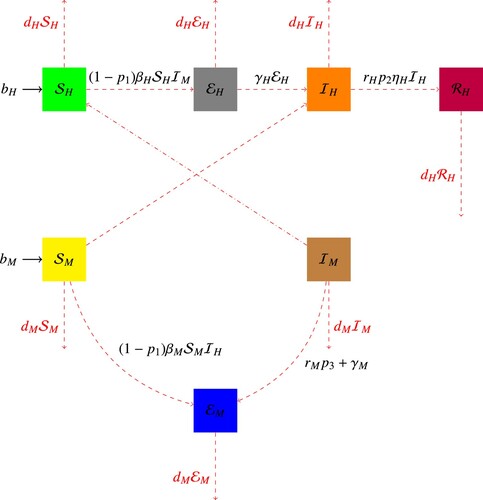
We reconsidered the dengue disease model [40] in the framework of piecewise differential and integral and analysed its crossover behaviours. The total population we divided into two categories, first in terms of the human population ${\mathcal{N}}_H$, there are four categories: Susceptible ${\mathcal{S}}_H$, Exposed ${\mathcal{E}}_H$, Infected ${\mathcal{I}}_H$, and Recovered ${\mathcal{R}}_H$. The total mosquito population ${\mathcal{N}}_M$ is also segmented into three groups: Susceptible ${\mathcal{S}}_M$, Exposed ${\mathcal{E}}_M$, and Infected ${\mathcal{I}}_M$. We do not consider any recovered classes in the mosquito population because mosquitoes infected with dengue retain the virus throughout their lives. Three control functions are incorporated into the proposed model: two for humans and one for mosquitoes. Insect repellents or mosquito nets used to shield individuals from mosquito bites are indicated by the control $p_1$. Because of heightened public awareness, we introduced $(1-p_1)$ into the illness transmission rate to reduce infection rates. Using control $p_2$, the illness can be treated. The control $p_3$ represents mosquito-killing operations aimed at reducing mosquito populations. The considered model in the sense of piecewise derivative having singular and non-singular kernels with order $0<\nu \le 1,\zeta \in [0,T]$, can be expressed as follows: (1) $\begin{array}{rl}{}_0^{C\mathbb{ABC}}{\mathfrak{D}}_{\zeta }^{\nu }\left({\mathcal{S}}_H\right(\zeta \left)\right)& =b_H-(1-p_1){\text{β}}_H{\mathcal{S}}_H{\mathcal{I}}_M-d_H{\mathcal{S}}_H,\\ {}_0^{C\mathbb{ABC}}{\mathfrak{D}}_{\zeta }^{\nu }\left({\mathcal{E}}_H\right(\zeta \left)\right)& =(1-p_1){\text{β}}_H{\mathcal{S}}_H{\mathcal{I}}_M-(d_H+{\gamma }_H){\mathcal{E}}_H,\\ {}_0^{C\mathbb{ABC}}{\mathfrak{D}}_{\zeta }^{\nu }\left({\mathcal{I}}_H\right(\zeta \left)\right)& ={\gamma }_H{\mathcal{E}}_H-r_H{p}_2{\eta }_H{\mathcal{I}}_H-d_H{\mathcal{I}}_H,\\ {}_0^{C\mathbb{ABC}}{\mathfrak{D}}_{\zeta }^{\nu }\left({\mathcal{R}}_H\right(\zeta \left)\right)& =r_H{p}_2{\eta }_H{\mathcal{I}}_H-d_H{\mathcal{R}}_H,\\ {}_0^{C\mathbb{ABC}}{\mathfrak{D}}_{\zeta }^{\nu }\left({\mathcal{S}}_M\right(\zeta \left)\right)& =b_M-(1-p_1){\text{β}}_M{\mathcal{S}}_M{\mathcal{I}}_H\\ & -r_M{p}_3{\mathcal{S}}_M-d_M{\mathcal{S}}_M,\\ {}_0^{C\mathbb{ABC}}{\mathfrak{D}}_{\zeta }^{\nu }\left({\mathcal{E}}_M\right(\zeta \left)\right)& =(1-p_1){\text{β}}_M{\mathcal{S}}_M{\mathcal{I}}_H\\ & -(r_M{p}_3+{\gamma }_M+d_M){\mathcal{E}}_M,\\ {}_0^{C\mathbb{ABC}}{\mathfrak{D}}_{\zeta }^{\nu }\left({\mathcal{I}}_H\right(\zeta \left)\right)& ={\gamma }_M{\mathcal{E}}_M-(r_M{p}_3+d_M){\mathcal{I}}_M,\end{array}$(1) having initial conditions $\begin{array}{rl}& {\mathcal{S}}_H\left(0\right)={\mathcal{S}}_0>0,{\mathcal{E}}_H\left(0\right)={\mathcal{E}}_0\ge 0,{\mathcal{I}}_H\left(0\right)={\mathcal{I}}_0\ge 0,\\ & {\mathcal{R}}_H\left(0\right)={\mathcal{R}}_0\ge 0,{\mathcal{S}}_M\left(0\right)={\mathcal{S}}_0\ge 0,\\ & {\mathcal{E}}_M\left(0\right)={\mathcal{E}}_0\ge 0,{\mathcal{I}}_M\left(0\right)={\mathcal{I}}_0\ge 0.\end{array}$These parameters encapsulate key aspects of the population dynamics in the context of a disease such as dengue, commonly transmitted by mosquitoes. The birth rates of human (b_H) and mosquito (b_M) populations, along with their respective death rates (d_H and d_M), delineate the demographic changes in each group. Transmission rates, β_H and β_M, reflect the efficiency of the virus moving between mosquitoes and humans. Incubation rates, γ_H and γ_M, signify the pace at which the virus matures within each population. The recovery rate of the human population (η_H) and the proportion of effective dengue treatment (r_H) play vital roles in disease management. Additionally, mosquito killing efficiency (r_M) represents the impact of interventions on reducing the mosquito population, influencing the overall transmission dynamics. These parameters collectively contribute to modelling and comprehending the intricate interplay between populations and disease, crucial for devising effective strategies for disease control and prevention.

The flow chart diagram of the considered model is given in Figure 1. To describe equation (1(1) $\begin{array}{rl}{}_0^{C\mathbb{ABC}}{\mathfrak{D}}_{\zeta }^{\nu }\left({\mathcal{S}}_H\right(\zeta \left)\right)& =b_H-(1-p_1){\text{β}}_H{\mathcal{S}}_H{\mathcal{I}}_M-d_H{\mathcal{S}}_H,\\ {}_0^{C\mathbb{ABC}}{\mathfrak{D}}_{\zeta }^{\nu }\left({\mathcal{E}}_H\right(\zeta \left)\right)& =(1-p_1){\text{β}}_H{\mathcal{S}}_H{\mathcal{I}}_M-(d_H+{\gamma }_H){\mathcal{E}}_H,\\ {}_0^{C\mathbb{ABC}}{\mathfrak{D}}_{\zeta }^{\nu }\left({\mathcal{I}}_H\right(\zeta \left)\right)& ={\gamma }_H{\mathcal{E}}_H-r_H{p}_2{\eta }_H{\mathcal{I}}_H-d_H{\mathcal{I}}_H,\\ {}_0^{C\mathbb{ABC}}{\mathfrak{D}}_{\zeta }^{\nu }\left({\mathcal{R}}_H\right(\zeta \left)\right)& =r_H{p}_2{\eta }_H{\mathcal{I}}_H-d_H{\mathcal{R}}_H,\\ {}_0^{C\mathbb{ABC}}{\mathfrak{D}}_{\zeta }^{\nu }\left({\mathcal{S}}_M\right(\zeta \left)\right)& =b_M-(1-p_1){\text{β}}_M{\mathcal{S}}_M{\mathcal{I}}_H\\ & -r_M{p}_3{\mathcal{S}}_M-d_M{\mathcal{S}}_M,\\ {}_0^{C\mathbb{ABC}}{\mathfrak{D}}_{\zeta }^{\nu }\left({\mathcal{E}}_M\right(\zeta \left)\right)& =(1-p_1){\text{β}}_M{\mathcal{S}}_M{\mathcal{I}}_H\\ & -(r_M{p}_3+{\gamma }_M+d_M){\mathcal{E}}_M,\\ {}_0^{C\mathbb{ABC}}{\mathfrak{D}}_{\zeta }^{\nu }\left({\mathcal{I}}_H\right(\zeta \left)\right)& ={\gamma }_M{\mathcal{E}}_M-(r_M{p}_3+d_M){\mathcal{I}}_M,\end{array}$(1) ) more precisely, we can write it as follows: (2) $\begin{array}{r}\begin{array}{rl}& {}_0^{C\mathbb{ABC}}{\mathfrak{D}}_{\zeta }^{\nu }\left({\mathcal{S}}_H\right(\zeta \left)\right)\\ & =\{\begin{array}{ll}{}_0^C{\mathfrak{D}}_{\zeta }^{\nu }\left({\mathcal{S}}_H\right(\zeta \left)\right)={}^C{H}_1({\mathcal{S}}_H,\zeta ),& 0<\zeta \le {\zeta }_1,\\ {}_0^{\mathbb{ABC}}{\mathfrak{D}}_{\zeta }^{\nu }\left({\mathcal{S}}_H\right(\zeta \left)\right)={}^{\mathbb{ABC}}{H}_1({\mathcal{S}}_H,\zeta ),& {\zeta }_1<\zeta \le T,\end{array}\\ & {}_0^{C\mathbb{ABC}}{\mathfrak{D}}_{\zeta }^{\nu }\left({\mathcal{E}}_H\right(\zeta \left)\right)\\ & =\{\begin{array}{ll}{}_0^C{\mathfrak{D}}_{\zeta }^{\nu }\left({\mathcal{E}}_H\right(\zeta \left)\right)={}^C{H}_2({\mathcal{E}}_H,\zeta ),& 0<\zeta \le {\zeta }_1,\\ {}_0^{\mathbb{ABC}}{\mathfrak{D}}_{\zeta }^{\nu }\left({\mathcal{E}}_H\right(\zeta \left)\right)={}^{\mathbb{ABC}}{H}_2({\mathcal{E}}_H,\zeta ),& {\zeta }_1<\zeta \le T,\end{array}\\ & {}_0^{C\mathbb{ABC}}{\mathfrak{D}}_{\zeta }^{\nu }\left({\mathcal{I}}_H\right(\zeta \left)\right)\\ & =\{\begin{array}{ll}{}_0^C{\mathfrak{D}}_{\zeta }^{\nu }\left({\mathcal{I}}_H\right(\zeta \left)\right)={}^C{H}_3({\mathcal{I}}_H,\zeta ),& 0<\zeta \le {\zeta }_1,\\ {}_0^{\mathbb{ABC}}{\mathfrak{D}}_{\zeta }^{\nu }\left({\mathcal{I}}_H\right(\zeta \left)\right)={}^{\mathbb{ABC}}{H}_3({\mathcal{I}}_H,\zeta ),& {\zeta }_1<\zeta \le T,\end{array}\\ & {}_0^{C\mathbb{ABC}}{\mathfrak{D}}_{\zeta }^{\nu }\left({\mathcal{R}}_H\right(\zeta \left)\right)\\ & =\{\begin{array}{ll}{}_0^C{\mathfrak{D}}_{\zeta }^{\nu }\left({\mathcal{R}}_H\right(\zeta \left)\right)={}^C{H}_4({\mathcal{R}}_H,\zeta ),& 0<\zeta \le {\zeta }_1,\\ {}_0^{\mathbb{ABC}}{\mathfrak{D}}_{\zeta }^{\nu }\left({\mathcal{R}}_H\right(\zeta \left)\right)={}^{\mathbb{ABC}}{H}_4({\mathcal{R}}_H,\zeta ),& {\zeta }_1<\zeta \le T,\end{array}\\ & {}_0^{C\mathbb{ABC}}{\mathfrak{D}}_{\zeta }^{\nu }\left({\mathcal{S}}_M\right(\zeta \left)\right)\\ & =\{\begin{array}{ll}{}_0^C{\mathfrak{D}}_{\zeta }^{\nu }\left({\mathcal{S}}_M\right(\zeta \left)\right)={}^C{H}_5({\mathcal{S}}_M,\zeta ),& 0<\zeta \le {\zeta }_1,\\ {}_0^{\mathbb{ABC}}{\mathfrak{D}}_{\zeta }^{\nu }\left({\mathcal{S}}_M\right(\zeta \left)\right)={}^{\mathbb{ABC}}{H}_5({\mathcal{S}}_M,\zeta ),& {\zeta }_1<\zeta \le T,\end{array}\\ & {}_0^{C\mathbb{ABC}}{\mathfrak{D}}_{\zeta }^{\nu }\left({\mathcal{E}}_M\right(\zeta \left)\right)\\ & =\{\begin{array}{ll}{}_0^C{\mathfrak{D}}_{\zeta }^{\nu }\left({\mathcal{E}}_M\right(\zeta \left)\right)={}^C{H}_6({\mathcal{E}}_M,\zeta ),& 0<\zeta \le {\zeta }_1,\\ {}_0^{\mathbb{ABC}}{\mathfrak{D}}_{\zeta }^{\nu }\left({\mathcal{E}}_M\right(\zeta \left)\right)={}^{\mathbb{ABC}}{H}_6({\mathcal{E}}_M,\zeta ),& {\zeta }_1<\zeta \le T,\end{array}\\ & {}_0^{C\mathbb{ABC}}{\mathfrak{D}}_{\zeta }^{\nu }\left({\mathcal{I}}_M\right(\zeta \left)\right)\\ & =\{\begin{array}{ll}{}_0^C{\mathfrak{D}}_{\zeta }^{\nu }\left({\mathcal{I}}_M\right(\zeta \left)\right)={}^C{H}_7({\mathcal{I}}_M,\zeta ),& 0<\zeta \le {\zeta }_1,\\ {}_0^{\mathbb{ABC}}{\mathfrak{D}}_{\zeta }^{\nu }\left({\mathcal{I}}_M\right(\zeta \left)\right)={}^{\mathbb{ABC}}{H}_7({\mathcal{I}}_M,\zeta ),& {\zeta }_1<\zeta \le T,\end{array}\end{array}\end{array}$(2) where ${}_0^C{\mathfrak{D}}_{\zeta }^{\nu }$ and ${}_0^{C\mathbb{ABC}}{\mathfrak{D}}_{\zeta }^{\nu }$ are Caputo and $\mathbb{ABC}$ derivative, respectively.

Figure 1. Schematic diagram of the dengue model.

Motivated from the above literature a piecewise fractional operators are a useful tool for capturing crossover and abrupt dynamics in system dynamics, which is why we utilized them in our study. This paper examined a set of differential equations under the Caputo and Atangana–Baleanu piecewise fractional operator that characterizes the crossover dynamics of dengue model. In particular, we applied various fractional operators to various system intervals and offered a qualitative analysis for every subinterval. We employed the UH stability analysis to evaluate stability. In order to generate approximation solutions that can accommodate dynamics of both integer and rational orders, we also looked into the use of piecewise terms and fractional orders in the system's final step. The neural network approach is used and plotted the dynamics of the proposed model, respectively.

The rest of the work is organized as follows: In Section 2, we discuss the basic results used in the manuscript. The existence and uniqueness results are established by using the fixed point approach in Section 3. Numerical approach is analysed for the considered model (2(2) $\begin{array}{r}\begin{array}{rl}& {}_0^{C\mathbb{ABC}}{\mathfrak{D}}_{\zeta }^{\nu }\left({\mathcal{S}}_H\right(\zeta \left)\right)\\ & =\{\begin{array}{ll}{}_0^C{\mathfrak{D}}_{\zeta }^{\nu }\left({\mathcal{S}}_H\right(\zeta \left)\right)={}^C{H}_1({\mathcal{S}}_H,\zeta ),& 0<\zeta \le {\zeta }_1,\\ {}_0^{\mathbb{ABC}}{\mathfrak{D}}_{\zeta }^{\nu }\left({\mathcal{S}}_H\right(\zeta \left)\right)={}^{\mathbb{ABC}}{H}_1({\mathcal{S}}_H,\zeta ),& {\zeta }_1<\zeta \le T,\end{array}\\ & {}_0^{C\mathbb{ABC}}{\mathfrak{D}}_{\zeta }^{\nu }\left({\mathcal{E}}_H\right(\zeta \left)\right)\\ & =\{\begin{array}{ll}{}_0^C{\mathfrak{D}}_{\zeta }^{\nu }\left({\mathcal{E}}_H\right(\zeta \left)\right)={}^C{H}_2({\mathcal{E}}_H,\zeta ),& 0<\zeta \le {\zeta }_1,\\ {}_0^{\mathbb{ABC}}{\mathfrak{D}}_{\zeta }^{\nu }\left({\mathcal{E}}_H\right(\zeta \left)\right)={}^{\mathbb{ABC}}{H}_2({\mathcal{E}}_H,\zeta ),& {\zeta }_1<\zeta \le T,\end{array}\\ & {}_0^{C\mathbb{ABC}}{\mathfrak{D}}_{\zeta }^{\nu }\left({\mathcal{I}}_H\right(\zeta \left)\right)\\ & =\{\begin{array}{ll}{}_0^C{\mathfrak{D}}_{\zeta }^{\nu }\left({\mathcal{I}}_H\right(\zeta \left)\right)={}^C{H}_3({\mathcal{I}}_H,\zeta ),& 0<\zeta \le {\zeta }_1,\\ {}_0^{\mathbb{ABC}}{\mathfrak{D}}_{\zeta }^{\nu }\left({\mathcal{I}}_H\right(\zeta \left)\right)={}^{\mathbb{ABC}}{H}_3({\mathcal{I}}_H,\zeta ),& {\zeta }_1<\zeta \le T,\end{array}\\ & {}_0^{C\mathbb{ABC}}{\mathfrak{D}}_{\zeta }^{\nu }\left({\mathcal{R}}_H\right(\zeta \left)\right)\\ & =\{\begin{array}{ll}{}_0^C{\mathfrak{D}}_{\zeta }^{\nu }\left({\mathcal{R}}_H\right(\zeta \left)\right)={}^C{H}_4({\mathcal{R}}_H,\zeta ),& 0<\zeta \le {\zeta }_1,\\ {}_0^{\mathbb{ABC}}{\mathfrak{D}}_{\zeta }^{\nu }\left({\mathcal{R}}_H\right(\zeta \left)\right)={}^{\mathbb{ABC}}{H}_4({\mathcal{R}}_H,\zeta ),& {\zeta }_1<\zeta \le T,\end{array}\\ & {}_0^{C\mathbb{ABC}}{\mathfrak{D}}_{\zeta }^{\nu }\left({\mathcal{S}}_M\right(\zeta \left)\right)\\ & =\{\begin{array}{ll}{}_0^C{\mathfrak{D}}_{\zeta }^{\nu }\left({\mathcal{S}}_M\right(\zeta \left)\right)={}^C{H}_5({\mathcal{S}}_M,\zeta ),& 0<\zeta \le {\zeta }_1,\\ {}_0^{\mathbb{ABC}}{\mathfrak{D}}_{\zeta }^{\nu }\left({\mathcal{S}}_M\right(\zeta \left)\right)={}^{\mathbb{ABC}}{H}_5({\mathcal{S}}_M,\zeta ),& {\zeta }_1<\zeta \le T,\end{array}\\ & {}_0^{C\mathbb{ABC}}{\mathfrak{D}}_{\zeta }^{\nu }\left({\mathcal{E}}_M\right(\zeta \left)\right)\\ & =\{\begin{array}{ll}{}_0^C{\mathfrak{D}}_{\zeta }^{\nu }\left({\mathcal{E}}_M\right(\zeta \left)\right)={}^C{H}_6({\mathcal{E}}_M,\zeta ),& 0<\zeta \le {\zeta }_1,\\ {}_0^{\mathbb{ABC}}{\mathfrak{D}}_{\zeta }^{\nu }\left({\mathcal{E}}_M\right(\zeta \left)\right)={}^{\mathbb{ABC}}{H}_6({\mathcal{E}}_M,\zeta ),& {\zeta }_1<\zeta \le T,\end{array}\\ & {}_0^{C\mathbb{ABC}}{\mathfrak{D}}_{\zeta }^{\nu }\left({\mathcal{I}}_M\right(\zeta \left)\right)\\ & =\{\begin{array}{ll}{}_0^C{\mathfrak{D}}_{\zeta }^{\nu }\left({\mathcal{I}}_M\right(\zeta \left)\right)={}^C{H}_7({\mathcal{I}}_M,\zeta ),& 0<\zeta \le {\zeta }_1,\\ {}_0^{\mathbb{ABC}}{\mathfrak{D}}_{\zeta }^{\nu }\left({\mathcal{I}}_M\right(\zeta \left)\right)={}^{\mathbb{ABC}}{H}_7({\mathcal{I}}_M,\zeta ),& {\zeta }_1<\zeta \le T,\end{array}\end{array}\end{array}$(2) ) with fractional order in section Section 4. Simulation of the proposed model has been discussed along with DNN with datasets and mentioned different dynamics graphically in Section 5. Finally, we conclude our work in Section 6.

2. Basic results

Here we will give some preliminary definitions of Caputo and $\mathbb{ABC}$ fractional derivatives and integrals.

Definition 2.1

[15]

The derivative of a function $\mathbb{W}\left(\zeta \right)$ with respect to the $\mathbb{ABC}$ ( Atangana–Baleanu–Caputo) operator, given the condition that $\mathbb{W}\left(\zeta \right)$ belongs to the space ${\mathcal{H}}^1(0,\tau )$, is defined as follows: (3) $\begin{array}{rl}{}_0^{\mathbb{ABC}}{D}_{\zeta }^{\nu }\left(\mathbb{W}\right(\zeta \left)\right)& =\frac{\mathbb{ABC}\left(\nu \right)}{1-\nu }{\int }_0^{\zeta }\frac{\mathrm{d}}{\mathrm{d}\theta }\mathbb{W}\left(\theta \right)\\ & \times E_{\nu }[\frac{-\nu }{1-\nu }(\zeta -\theta {)}^{\nu }]\mathrm{d}\theta .\end{array}$(3) Replace $E_{\nu }\left[\frac{-\nu }{1-\nu }\right(\zeta -\theta {)}^{\theta }]$ with $E_1=\exp \left[\frac{-\nu }{1-\nu }\right(\zeta -\theta \left)\right]$ in Equation (3(3) $\begin{array}{rl}{}_0^{\mathbb{ABC}}{D}_{\zeta }^{\nu }\left(\mathbb{W}\right(\zeta \left)\right)& =\frac{\mathbb{ABC}\left(\nu \right)}{1-\nu }{\int }_0^{\zeta }\frac{\mathrm{d}}{\mathrm{d}\theta }\mathbb{W}\left(\theta \right)\\ & \times E_{\nu }[\frac{-\nu }{1-\nu }(\zeta -\theta {)}^{\nu }]\mathrm{d}\theta .\end{array}$(3) ) to obtain the Caputo–Fabrizio differential operator. Additionally, it is noted that ${}_0^{\mathbb{ABC}}{D}_{\zeta }^{\nu }\left[\mathrm{constant}\right]=0$. In this context, the normalization operator denoted as $\mathcal{ABC}\left(\nu \right)$ is expressed as $\mathbb{ABC}\left(0\right)=\mathbb{ABC}\left(1\right)=1$. Additionally, the symbol $K_{\nu }$ signifies the Mittag–Leffler function, which is a generalized form of the exponential function.

Definition 2.2

[15]

If $\mathbb{W}\left(t\right)\in L[0,T]$, then the fractional integral in the $\mathbb{ABC}$ sense is expressed as: (4) $\begin{array}{rl}{}_0^{\mathbb{ABC}}{I}_{\zeta }^{\nu }\mathbb{W}\left(\zeta \right)& =\frac{1-\nu }{\mathbb{ABC}\left(\nu \right)}\mathbb{W}\left(\zeta \right)+\frac{\nu }{\mathbb{ABC}\left(\nu \right)\mathrm{\Gamma }\left(\nu \right)}\\ & \times {\int }_0^{\zeta }(\zeta -\theta {)}^{\nu -1}\mathbb{W}(\theta )\mathrm{d}\theta .\end{array}$(4)

Definition 2.3

[16]

Consider the function $\mathbb{W}\left(\zeta \right)$. For the definition of the arbitrary order derivative in the Caputo sense with respect to ζ, it is expressed as: $\begin{array}{r}{}_0^C{D}_{\zeta }^{\nu }\mathbb{W}\left(\zeta \right)=\frac{1}{\mathrm{\Gamma }(1-\nu )}{\int }_0^{\zeta }(\zeta -\theta {)}^{-\nu }[\mathbb{W}{}^{\prime }\left(\theta \right)]\mathrm{d}\theta .\end{array}$where $\mathrm{\Gamma }(.)$ represents the gamma function.

Definition 2.4

Consider the function $\mathbb{W}\left(\zeta \right)$ to be differentiable. For the definition of Caputo and $\mathbb{ABC}$ fractional piecewise derivative, as introduced in Ref. [15], it is expressed as: $\begin{array}{r}{}_0^{\mathrm{PC}\mathbb{ABC}}{D}_{\zeta }^{\nu }\mathbb{W}\left(\zeta \right)=\{\begin{array}{ll}{}_0^C{D}_{\zeta }^{\nu }\mathbb{W}\left(\zeta \right),& 0<t\le {\zeta }_1,\\ {}_0^{\mathbb{ABC}}{D}_{\zeta }^{\nu }\mathbb{W}\left(\zeta \right)& {\zeta }_1<\zeta \le T,\end{array}\end{array}$here, ${}^{\mathrm{PC}\mathbb{ABC}}0D{\zeta }^{\nu }\mathbb{W}\left(\zeta \right)$ represents the Caputo derivative for $0<\zeta \le {\zeta }_1$ and the fractional $\mathbb{ABC}$ derivative for ${\zeta }_1<\zeta \le T$.

Definition 2.5

Consider the function $\mathbb{W}\left(\zeta \right)$ to be differentiable. For the definition of fractional Caputo and fractional $\mathbb{ABC}$ piecewise integration, as introduced in [15], it is expressed as: $\begin{array}{rl}& {}_0^{\mathrm{PC}\mathbb{ABC}}{I}_{\zeta }\mathbb{W}\left(\zeta \right)\\ & =\{\begin{array}{ll}\frac{1}{\mathrm{\Gamma }\nu }{\int }_{{\zeta }_1}^{\zeta }(\zeta -\theta {)}^{\nu -1}\mathbb{W}(\theta \left)d\right(\theta ),& 0<t\le {\zeta }_1,\\ \begin{array}{l}\frac{1-\nu }{\mathbb{ABC}\left(\nu \right)}\mathbb{W}\left(\zeta \right)+\frac{\nu }{\mathbb{ABC}\left(\nu \right)\mathrm{\Gamma }\nu }\\ \times {\int }_{{\zeta }_1}^{\zeta }(\zeta -\nu {)}^{\nu -1}\mathbb{W}(\theta \left)d\right(\theta )\end{array}& {\zeta }_1<\zeta \le T,\end{array}\end{array}$here, ${}^{\mathrm{PC}\mathbb{ABC}}0I\zeta \mathbb{W}\left(\zeta \right)$ denotes Caputo singular kernel integration for $0<\zeta \le {\zeta }_1$ and $\mathbb{ABC}$ integration for ${\zeta }_1<\zeta \le T$.

3. Qualitative analysis

Lemma 2.6

Now, we want to prove the existence and uniqueness of the solution for the considered piecewise derivable function. We can use the system (2(2) $\begin{array}{r}\begin{array}{rl}& {}_0^{C\mathbb{ABC}}{\mathfrak{D}}_{\zeta }^{\nu }\left({\mathcal{S}}_H\right(\zeta \left)\right)\\ & =\{\begin{array}{ll}{}_0^C{\mathfrak{D}}_{\zeta }^{\nu }\left({\mathcal{S}}_H\right(\zeta \left)\right)={}^C{H}_1({\mathcal{S}}_H,\zeta ),& 0<\zeta \le {\zeta }_1,\\ {}_0^{\mathbb{ABC}}{\mathfrak{D}}_{\zeta }^{\nu }\left({\mathcal{S}}_H\right(\zeta \left)\right)={}^{\mathbb{ABC}}{H}_1({\mathcal{S}}_H,\zeta ),& {\zeta }_1<\zeta \le T,\end{array}\\ & {}_0^{C\mathbb{ABC}}{\mathfrak{D}}_{\zeta }^{\nu }\left({\mathcal{E}}_H\right(\zeta \left)\right)\\ & =\{\begin{array}{ll}{}_0^C{\mathfrak{D}}_{\zeta }^{\nu }\left({\mathcal{E}}_H\right(\zeta \left)\right)={}^C{H}_2({\mathcal{E}}_H,\zeta ),& 0<\zeta \le {\zeta }_1,\\ {}_0^{\mathbb{ABC}}{\mathfrak{D}}_{\zeta }^{\nu }\left({\mathcal{E}}_H\right(\zeta \left)\right)={}^{\mathbb{ABC}}{H}_2({\mathcal{E}}_H,\zeta ),& {\zeta }_1<\zeta \le T,\end{array}\\ & {}_0^{C\mathbb{ABC}}{\mathfrak{D}}_{\zeta }^{\nu }\left({\mathcal{I}}_H\right(\zeta \left)\right)\\ & =\{\begin{array}{ll}{}_0^C{\mathfrak{D}}_{\zeta }^{\nu }\left({\mathcal{I}}_H\right(\zeta \left)\right)={}^C{H}_3({\mathcal{I}}_H,\zeta ),& 0<\zeta \le {\zeta }_1,\\ {}_0^{\mathbb{ABC}}{\mathfrak{D}}_{\zeta }^{\nu }\left({\mathcal{I}}_H\right(\zeta \left)\right)={}^{\mathbb{ABC}}{H}_3({\mathcal{I}}_H,\zeta ),& {\zeta }_1<\zeta \le T,\end{array}\\ & {}_0^{C\mathbb{ABC}}{\mathfrak{D}}_{\zeta }^{\nu }\left({\mathcal{R}}_H\right(\zeta \left)\right)\\ & =\{\begin{array}{ll}{}_0^C{\mathfrak{D}}_{\zeta }^{\nu }\left({\mathcal{R}}_H\right(\zeta \left)\right)={}^C{H}_4({\mathcal{R}}_H,\zeta ),& 0<\zeta \le {\zeta }_1,\\ {}_0^{\mathbb{ABC}}{\mathfrak{D}}_{\zeta }^{\nu }\left({\mathcal{R}}_H\right(\zeta \left)\right)={}^{\mathbb{ABC}}{H}_4({\mathcal{R}}_H,\zeta ),& {\zeta }_1<\zeta \le T,\end{array}\\ & {}_0^{C\mathbb{ABC}}{\mathfrak{D}}_{\zeta }^{\nu }\left({\mathcal{S}}_M\right(\zeta \left)\right)\\ & =\{\begin{array}{ll}{}_0^C{\mathfrak{D}}_{\zeta }^{\nu }\left({\mathcal{S}}_M\right(\zeta \left)\right)={}^C{H}_5({\mathcal{S}}_M,\zeta ),& 0<\zeta \le {\zeta }_1,\\ {}_0^{\mathbb{ABC}}{\mathfrak{D}}_{\zeta }^{\nu }\left({\mathcal{S}}_M\right(\zeta \left)\right)={}^{\mathbb{ABC}}{H}_5({\mathcal{S}}_M,\zeta ),& {\zeta }_1<\zeta \le T,\end{array}\\ & {}_0^{C\mathbb{ABC}}{\mathfrak{D}}_{\zeta }^{\nu }\left({\mathcal{E}}_M\right(\zeta \left)\right)\\ & =\{\begin{array}{ll}{}_0^C{\mathfrak{D}}_{\zeta }^{\nu }\left({\mathcal{E}}_M\right(\zeta \left)\right)={}^C{H}_6({\mathcal{E}}_M,\zeta ),& 0<\zeta \le {\zeta }_1,\\ {}_0^{\mathbb{ABC}}{\mathfrak{D}}_{\zeta }^{\nu }\left({\mathcal{E}}_M\right(\zeta \left)\right)={}^{\mathbb{ABC}}{H}_6({\mathcal{E}}_M,\zeta ),& {\zeta }_1<\zeta \le T,\end{array}\\ & {}_0^{C\mathbb{ABC}}{\mathfrak{D}}_{\zeta }^{\nu }\left({\mathcal{I}}_M\right(\zeta \left)\right)\\ & =\{\begin{array}{ll}{}_0^C{\mathfrak{D}}_{\zeta }^{\nu }\left({\mathcal{I}}_M\right(\zeta \left)\right)={}^C{H}_7({\mathcal{I}}_M,\zeta ),& 0<\zeta \le {\zeta }_1,\\ {}_0^{\mathbb{ABC}}{\mathfrak{D}}_{\zeta }^{\nu }\left({\mathcal{I}}_M\right(\zeta \left)\right)={}^{\mathbb{ABC}}{H}_7({\mathcal{I}}_M,\zeta ),& {\zeta }_1<\zeta \le T,\end{array}\end{array}\end{array}$(2) ) as described in Lemma 2.6 to achieve this. Further elaborating on this, we can write it as follows: $\begin{array}{r}{}_0^{\mathrm{AC}\mathbb{ABC}}{D}_{\zeta }^{\nu }\mathbb{W}\left(\zeta \right)=H(\zeta ,\mathbb{W}(\mathrm{t\zeta }\left)\right),0<\nu \le 1,\end{array}$is (5) $\begin{array}{r}\mathbb{W}\left(\zeta \right)=\{\begin{array}{ll}\begin{array}{l}{\mathbb{W}}_0+\frac{1}{\mathrm{\Gamma }\left(\nu \right)}{\int }_0^{\zeta }\mathrm{\zeta H}(\theta ,\mathbb{W}(\theta \left)\right)\\ \times (\zeta -\theta {)}^{\nu -1}\mathrm{d}\theta ,\end{array}& 0<\zeta \le {\zeta }_1\\ \begin{array}{l}\mathbb{W}\left({\zeta }_1\right)+\frac{1-\nu }{\mathbb{ABC}\left(\nu \right)}H(\zeta ,\mathbb{W}(\zeta \left)\right)\\ +\frac{\nu }{\mathbb{ABC}\left(\nu \right)\mathrm{\Gamma }\nu }{\int }_{{\zeta }_1}^{\zeta }(\zeta -\theta {)}^{\theta -1}\\ \times H(\theta ,\mathbb{W}(\theta \left)\right)d\left(\theta \right),\end{array}& {\zeta }_1<\zeta \le T,\end{array}\end{array}$(5)

where (6) $\begin{array}{rl}& \mathbb{W}\left(\zeta \right)=\{\begin{array}{l}{\mathcal{S}}_H\left(\zeta \right)\\ {\mathcal{E}}_H\left(\zeta \right)\\ {\mathcal{I}}_H\left(\zeta \right)\\ {\mathcal{R}}_H\left(\zeta \right)\\ {\mathcal{S}}_M\left(\zeta \right)\\ {\mathcal{E}}_M\left(\zeta \right)\\ {\mathcal{I}}_M\left(\zeta \right)\end{array}{\mathbb{W}}_0=\{\begin{array}{l}{\mathcal{S}}_{H\left(0\right)}\\ {\mathcal{E}}_{H\left(0\right)}\\ {\mathcal{I}}_{H\left(0\right)}\\ {\mathcal{R}}_{H\left(0\right)}\\ {\mathcal{S}}_{M\left(0\right)}\\ {\mathcal{E}}_{M\left(0\right)}\\ {\mathcal{I}}_{M\left(0\right)}\end{array}{\mathbb{W}}_{\left({\zeta }_1\right)}=\{\begin{array}{l}{\mathcal{S}}_{H\left({\zeta }_1\right)}\\ {\mathcal{E}}_{H\left({\zeta }_1\right)}\\ {\mathcal{I}}_{H\left({\zeta }_1\right)}\\ {\mathcal{R}}_{H\left({\zeta }_1\right)}\\ {\mathcal{S}}_{M\left({\zeta }_1\right)}\\ {\mathcal{E}}_{M\left({\zeta }_1\right)}\\ {\mathcal{I}}_{M\left({\zeta }_1\right)}\end{array}\\ & Q(\zeta ,\mathbb{W}(\zeta \left)\right)\\ & =\{\begin{array}{l}{H}_i=\{\begin{array}{l}{}^C{H}_i({\mathcal{S}}_H,{\mathcal{E}}_H,{\mathcal{I}}_H,{\mathcal{R}}_H,{\mathcal{S}}_M,{\mathcal{E}}_M,{\mathcal{I}}_M,\zeta )\\ {}^{\mathbb{ABC}}{H}_i({\mathcal{S}}_H,{\mathcal{E}}_H,{\mathcal{I}}_H,{\mathcal{R}}_H,{\mathcal{S}}_M,{\mathcal{E}}_M,{\mathcal{I}}_M,\zeta )\end{array}\end{array},\end{array}$(6) where, i = 1, 2, 3, 4, 5, 6, 7 now we take $\mathrm{\infty }>T\ge \zeta >0$ then $X=\left(C\right[0,T]\times R^7,R_{+})$ is a Banach space. Further, $M=X_1\times X_2\times X_3\times X_4\times X_5\times X_6\times X_7$ is also complete norm space endowed with norm $\begin{array}{rl}\Vert \mathbb{W}\Vert & =\underset{\zeta \in [0,T]}{max}|\mathbb{W}\left(\zeta \right)|\\ & =\underset{\zeta \in [0,T]}{sup}\left[|\mathbb{S}\right(\zeta )|+|\mathbb{E}(\zeta )|+|\mathbb{I}(\zeta )|+|\mathbb{A}(\zeta )|\\ & +|\mathbb{H}\left(\zeta \right)|+|\mathbb{R}\left(\zeta \right)|+|\mathbb{W}\left(\zeta \right)|],\end{array}$which can be written as in equation (18(18) $\begin{array}{rl}& \left|\left|F\right(\mathbb{W})-F(\overline{\mathbb{W}}\left)\right|\right|\\ & \le \{\begin{array}{ll}\frac{{\mathcal{T}}_1^{\nu }}{\mathrm{\Gamma }(\nu +1)}\text{ß},& \zeta \in {\mathcal{T}}_1\\ \left[\frac{(1-\nu )\mathrm{\Gamma }\left(\nu \right)+\left(T_2^{\nu }\right)}{\mathrm{ABC}\left(\nu \right)\mathrm{\Gamma }\left(\nu \right)}\right]\text{ß}=\mathrm{\Lambda }\text{ß},& \zeta \in {\mathcal{T}}_2.\end{array}\end{array}$(18) ).

To get the required result, we consider the growth condition on the non-linear operator as:

(C1)	∃$L_{\mathbb{W}}>0$; ∀$K,\overline{\mathbb{W}}\in K$ we have $\begin{array}{r}|K(\zeta ,\mathbb{W})-K(\zeta ,\overline{\mathbb{W}})|\le L_K|\mathbb{W}-\overline{\mathbb{W}}|\mathit{,}\end{array}$
(C2)	∃$C_K>0$$\mathrm{\&}$$M_K>0,$; $\begin{array}{r}|K(\zeta ,\mathbb{W}(\zeta \left)\right)|\le C_K|\mathbb{W}|+M_K.\end{array}$

Theorem 3.1

If H is piecewise continuous on the sub-intervals $0<\zeta \le {\zeta }_1$ and ${\zeta }_1<\zeta \le T$ within the interval $[0,T]$, and it also satisfies condition $\left(C2\right)$, then the piecewise problem (2(2) $\begin{array}{r}\begin{array}{rl}& {}_0^{C\mathbb{ABC}}{\mathfrak{D}}_{\zeta }^{\nu }\left({\mathcal{S}}_H\right(\zeta \left)\right)\\ & =\{\begin{array}{ll}{}_0^C{\mathfrak{D}}_{\zeta }^{\nu }\left({\mathcal{S}}_H\right(\zeta \left)\right)={}^C{H}_1({\mathcal{S}}_H,\zeta ),& 0<\zeta \le {\zeta }_1,\\ {}_0^{\mathbb{ABC}}{\mathfrak{D}}_{\zeta }^{\nu }\left({\mathcal{S}}_H\right(\zeta \left)\right)={}^{\mathbb{ABC}}{H}_1({\mathcal{S}}_H,\zeta ),& {\zeta }_1<\zeta \le T,\end{array}\\ & {}_0^{C\mathbb{ABC}}{\mathfrak{D}}_{\zeta }^{\nu }\left({\mathcal{E}}_H\right(\zeta \left)\right)\\ & =\{\begin{array}{ll}{}_0^C{\mathfrak{D}}_{\zeta }^{\nu }\left({\mathcal{E}}_H\right(\zeta \left)\right)={}^C{H}_2({\mathcal{E}}_H,\zeta ),& 0<\zeta \le {\zeta }_1,\\ {}_0^{\mathbb{ABC}}{\mathfrak{D}}_{\zeta }^{\nu }\left({\mathcal{E}}_H\right(\zeta \left)\right)={}^{\mathbb{ABC}}{H}_2({\mathcal{E}}_H,\zeta ),& {\zeta }_1<\zeta \le T,\end{array}\\ & {}_0^{C\mathbb{ABC}}{\mathfrak{D}}_{\zeta }^{\nu }\left({\mathcal{I}}_H\right(\zeta \left)\right)\\ & =\{\begin{array}{ll}{}_0^C{\mathfrak{D}}_{\zeta }^{\nu }\left({\mathcal{I}}_H\right(\zeta \left)\right)={}^C{H}_3({\mathcal{I}}_H,\zeta ),& 0<\zeta \le {\zeta }_1,\\ {}_0^{\mathbb{ABC}}{\mathfrak{D}}_{\zeta }^{\nu }\left({\mathcal{I}}_H\right(\zeta \left)\right)={}^{\mathbb{ABC}}{H}_3({\mathcal{I}}_H,\zeta ),& {\zeta }_1<\zeta \le T,\end{array}\\ & {}_0^{C\mathbb{ABC}}{\mathfrak{D}}_{\zeta }^{\nu }\left({\mathcal{R}}_H\right(\zeta \left)\right)\\ & =\{\begin{array}{ll}{}_0^C{\mathfrak{D}}_{\zeta }^{\nu }\left({\mathcal{R}}_H\right(\zeta \left)\right)={}^C{H}_4({\mathcal{R}}_H,\zeta ),& 0<\zeta \le {\zeta }_1,\\ {}_0^{\mathbb{ABC}}{\mathfrak{D}}_{\zeta }^{\nu }\left({\mathcal{R}}_H\right(\zeta \left)\right)={}^{\mathbb{ABC}}{H}_4({\mathcal{R}}_H,\zeta ),& {\zeta }_1<\zeta \le T,\end{array}\\ & {}_0^{C\mathbb{ABC}}{\mathfrak{D}}_{\zeta }^{\nu }\left({\mathcal{S}}_M\right(\zeta \left)\right)\\ & =\{\begin{array}{ll}{}_0^C{\mathfrak{D}}_{\zeta }^{\nu }\left({\mathcal{S}}_M\right(\zeta \left)\right)={}^C{H}_5({\mathcal{S}}_M,\zeta ),& 0<\zeta \le {\zeta }_1,\\ {}_0^{\mathbb{ABC}}{\mathfrak{D}}_{\zeta }^{\nu }\left({\mathcal{S}}_M\right(\zeta \left)\right)={}^{\mathbb{ABC}}{H}_5({\mathcal{S}}_M,\zeta ),& {\zeta }_1<\zeta \le T,\end{array}\\ & {}_0^{C\mathbb{ABC}}{\mathfrak{D}}_{\zeta }^{\nu }\left({\mathcal{E}}_M\right(\zeta \left)\right)\\ & =\{\begin{array}{ll}{}_0^C{\mathfrak{D}}_{\zeta }^{\nu }\left({\mathcal{E}}_M\right(\zeta \left)\right)={}^C{H}_6({\mathcal{E}}_M,\zeta ),& 0<\zeta \le {\zeta }_1,\\ {}_0^{\mathbb{ABC}}{\mathfrak{D}}_{\zeta }^{\nu }\left({\mathcal{E}}_M\right(\zeta \left)\right)={}^{\mathbb{ABC}}{H}_6({\mathcal{E}}_M,\zeta ),& {\zeta }_1<\zeta \le T,\end{array}\\ & {}_0^{C\mathbb{ABC}}{\mathfrak{D}}_{\zeta }^{\nu }\left({\mathcal{I}}_M\right(\zeta \left)\right)\\ & =\{\begin{array}{ll}{}_0^C{\mathfrak{D}}_{\zeta }^{\nu }\left({\mathcal{I}}_M\right(\zeta \left)\right)={}^C{H}_7({\mathcal{I}}_M,\zeta ),& 0<\zeta \le {\zeta }_1,\\ {}_0^{\mathbb{ABC}}{\mathfrak{D}}_{\zeta }^{\nu }\left({\mathcal{I}}_M\right(\zeta \left)\right)={}^{\mathbb{ABC}}{H}_7({\mathcal{I}}_M,\zeta ),& {\zeta }_1<\zeta \le T,\end{array}\end{array}\end{array}$(2) ) has at least one solution on each sub-interval.

Proof.

By applying the Schauder fixed-point theorem, let us define a closed subset in both subintervals of 0 to T as $G$ of $E$, as follows: $\begin{array}{r}G=\{\mathbb{W}\in K:\Vert \mathbb{W}\Vert \le R_{1,2},R>0\},\end{array}$Next, we introduce an operator, as follows: $\mathcal{T}:G\to G$ and applying (18(18) $\begin{array}{rl}& \left|\left|F\right(\mathbb{W})-F(\overline{\mathbb{W}}\left)\right|\right|\\ & \le \{\begin{array}{ll}\frac{{\mathcal{T}}_1^{\nu }}{\mathrm{\Gamma }(\nu +1)}\text{ß},& \zeta \in {\mathcal{T}}_1\\ \left[\frac{(1-\nu )\mathrm{\Gamma }\left(\nu \right)+\left(T_2^{\nu }\right)}{\mathrm{ABC}\left(\nu \right)\mathrm{\Gamma }\left(\nu \right)}\right]\text{ß}=\mathrm{\Lambda }\text{ß},& \zeta \in {\mathcal{T}}_2.\end{array}\end{array}$(18) ) as (7) $\begin{array}{r}\mathcal{T}\left(\mathbb{W}\right)=\{\begin{array}{ll}\begin{array}{l}{\mathbb{W}}_0+\frac{1}{\mathrm{\Gamma }\left(\nu \right)}{\int }_0^{{\zeta }_1}H(\theta ,\mathbb{W}(\theta \left)\right)\\ \times (\zeta -\theta {)}^{\theta -1}\mathrm{d}\theta ,\end{array}& 0<\zeta \le {\zeta }_1\\ \begin{array}{l}\mathbb{W}\left({\zeta }_1\right)+\frac{1-\nu }{\mathbb{ABC}\left(\nu \right)}H(\zeta ,\mathbb{W}(\zeta \left)\right)\\ +\frac{\nu }{\mathbb{ABC}\left(\nu \right)\mathrm{\Gamma }\left(\nu \right)}{\int }_{{\zeta }_1}^{\zeta }(\zeta -\theta {)}^{\theta -1}\\ \times H(\theta ,\mathbb{W}(\theta \left)\right)d\left(\theta \right),\end{array}& {\zeta }_1<\zeta \le T,\end{array}\end{array}$(7)

on any $\mathbb{W}\in G$, we get $\begin{array}{rl}& |\mathcal{T}\left(\mathbb{W}\right)\left(\zeta \right)|\\ & \le \{\begin{array}{l}|{\mathbb{W}}_0|+\frac{1}{\mathrm{\Gamma }\left(\nu \right)}{\int }_0^{{\zeta }_1}(\zeta -\theta {)}^{\nu -1}|H(\theta ,\mathbb{W}\left(\theta \right))|\mathrm{d}\theta ,\\ \begin{array}{l}|{\mathbb{W}}_{(}{\zeta }_1)|+\frac{1-\nu }{\mathbb{ABC}\left(\nu \right)}|H(\zeta ,\mathbb{W}\left(\zeta \right))|\\ +\frac{\nu }{\mathbb{ABC}\left(\nu \right)\mathrm{\Gamma }\left(\nu \right)}{\int }_{{\zeta }_1}^{\zeta }(\zeta -\theta {)}^{\nu -1}|H(\theta ,\mathbb{W}\left(\theta \right)\left)|d\right(\theta ),\end{array}\end{array}\\ & \le \{\begin{array}{l}|{\mathbb{W}}_0|+\frac{1}{\mathrm{\Gamma }\left(\nu \right)}{\int }_0^{{\zeta }_1}(\zeta -\theta {)}^{\nu -1}[C_H|\mathbb{W}|+M_H]\mathrm{d}\theta ,\\ \begin{array}{l}|{\mathbb{W}}_{(}{\zeta }_1)|+\frac{1-\nu }{\mathbb{ABC}\left(\nu \right)}[C_H|\mathbb{W}|+M_H]\\ +\frac{\nu }{\mathbb{ABC}\left(\nu \right)\mathrm{\Gamma }\left(\nu \right)}{\int }_{{\zeta }_1}^{\zeta }(\zeta -\theta {)}^{\nu -1}[C_H|\mathbb{W}|+M_H\left]d\right(\theta ),\end{array}\end{array}\\ & \le \{\begin{array}{ll}|{\mathbb{W}}_0|+\frac{{\mathbf{T}}^{\nu }}{\mathrm{\Gamma }(\nu +1)}[C_H|\mathbb{W}|+M_H]=R_1,& 0<\zeta \le {\zeta }_1,\\ \begin{array}{l}|{\mathbb{W}}_{(}{\zeta }_1)|+\frac{1-\nu }{\mathbb{ABC}\left(\nu \right)}[C_H|\mathbb{W}|+M_H]\\ +\frac{\sigma (T-\mathbf{T}{)}^{\nu }}{\mathbb{ABC}\left(\nu \right)\mathrm{\Gamma }\left(\nu +1\right)}[C_H|\mathbb{W}|\\ +M_H\left]d\right(\theta )=R_2,\end{array}& {\zeta }_1<\zeta \le T,\end{array}\\ & \le \{\begin{array}{ll}{R}_1,& 0<\zeta \le {\zeta }_1,\\ R_2,& {\zeta }_1<\zeta \le T.\end{array}\end{array}$From the last equation, as $\mathbb{W}\in G$. Thus $\mathcal{T}\left(G\right)\subset G$. Hence proves that $\mathcal{T}$ is complete and close. Further for complete continuity we write as Take ${\zeta }_z<{\zeta }_j\in [0,{\zeta }_1]$ first interval of the Caputo sense, assume (8) $\begin{array}{rl}& |\mathcal{T}\left(\mathbb{W}\right)\left({\zeta }_j\right)-\mathcal{T}\left(\mathbb{W}\right)\left({\zeta }_z\right)|\\ & =|\frac{1}{\mathrm{\Gamma }\left(\nu \right)}{\int }_0^{{\zeta }_j}({\zeta }_j-\theta {)}^{\nu -1}H(\theta ,\mathbb{W}\left(\theta \right))\mathrm{d}\theta \\ & -\frac{1}{\mathrm{\Gamma }\left(\nu \right)}{\int }_0^{{\zeta }_z}({\zeta }_z-\theta {)}^{\nu -1}H(\theta ,\mathbb{W}\left(\theta \right))\mathrm{d}\theta |\\ & \le \frac{1}{\mathrm{\Gamma }\left(\nu \right)}{\int }_0^{{\zeta }_z}\left[\right({\zeta }_z-\theta {)}^{\nu -1}-({\zeta }_j-\theta {)}^{\nu -1}]\\ & \times |H(\theta ,\mathbb{W}(\theta \left)\right)|\mathrm{d}\theta \\ & +\frac{1}{\mathrm{\Gamma }\left(\nu \right)}{\int }_{{\zeta }_i}^{{\zeta }_j}({\zeta }_j-\theta {)}^{\nu -1}|H(\theta ,\mathbb{W}\left(\theta \right))|\mathrm{d}\theta \\ & \le \frac{1}{\mathrm{\Gamma }\left(\nu \right)}[{\int }_0^{{\zeta }_i}\left[\right({\zeta }_z-\theta {)}^{\nu -1}-({\zeta }_j-\theta {)}^{\nu -1}]\mathrm{d}\theta \\ & +{\int }_{{\zeta }_z}^{{\zeta }_j}({\zeta }_j-\theta {)}^{\nu -1}\mathrm{d}\theta ](C_H|\mathbb{W}|+M_H)\\ & \le \frac{(C_H\mathbb{W}+M_H)}{\mathrm{\Gamma }(\nu +1)}[{\zeta }_j^{\nu }-{\zeta }_z^{\nu }+2({\zeta }_j-{\zeta }_z{)}^{\nu }].\end{array}$(8) Next (8), we get ${\zeta }_z\to {\zeta }_j$, then $\begin{array}{r}|\mathcal{T}\left(\mathbb{W}\right)\left({\zeta }_j\right)-\mathcal{T}\left(\mathbb{W}\right)\left({\zeta }_z\right)|\to 0,\mathrm{as}{\zeta }_z\to {\zeta }_j.\end{array}$So $\mathcal{T}$ is equi-continuous in $[0,{\zeta }_1]$ interval. Next we take the other interval ${\zeta }_z,{\zeta }_j\in [{\zeta }_1,T]$ in the $\mathbb{ABC}$ sense as (9) $\begin{array}{rl}& |\mathcal{T}\left(\mathbb{W}\right)\left({\zeta }_j\right)-\mathcal{T}\left(\mathbb{W}\right)\left({\zeta }_z\right)|\\ & =|\frac{1-\nu }{\mathbb{ABC}\left(\nu \right)}H(t,\mathbb{W}(t\left)\right)+\frac{\nu }{\mathbb{ABC}\left(\nu \right)\mathrm{\Gamma }\left(\nu \right)}\\ & \times {\int }_{{\zeta }_1}^{{\zeta }_j}({\zeta }_j-\theta {)}^{\nu -1}H(\theta ,\mathbb{W}\left(\theta \right))\mathrm{d}\theta ,\\ & -\frac{1-\nu }{\mathbb{ABC}\left(\nu \right)}H(\zeta ,\mathbb{W}(\zeta \left)\right)+\frac{\left(\nu \right)}{\mathbb{ABC}\left(\nu \right)\mathrm{\Gamma }\left(\nu \right)}\\ & \times {\int }_{{\zeta }_1}^{{\zeta }_z}({\zeta }_z-\theta {)}^{\nu -1}H(\theta ,\mathbb{W}\left(\theta \right))\mathrm{d}\theta |\\ & \le \frac{\nu }{\mathbb{ABC}\left(\nu \right)\mathrm{\Gamma }\left(\nu \right)}{\int }_{{\zeta }_1}^{{\zeta }_z}\left[\right({\zeta }_z-\theta {)}^{\nu -1}-({\zeta }_j-\theta {)}^{\nu -1}]\\ & \times |H(\theta ,\mathbb{W}(\theta \left)\right)|\mathrm{d}\theta \\ & +\frac{\nu }{\mathbb{ABC}\left(\nu \right)\mathrm{\Gamma }\left(\nu \right)}{\int }_{{\zeta }_z}^{{\zeta }_j}({\zeta }_j-\theta {)}^{\nu -1}|H(\theta ,\mathbb{W}\left(\theta \right))|\mathrm{d}\theta \\ & \le \frac{\nu }{\mathbb{ABC}\left(\nu \right)\mathrm{\Gamma }\left(\nu \right)}[{\int }_{{\zeta }_1}^{{\zeta }_z}\left[\right({\zeta }_z-\theta {)}^{\nu -1}-({\zeta }_j-\theta {)}^{\nu -1}]\mathrm{d}\theta \\ & +{\int }_{{\zeta }_z}^{{\zeta }_j}({\zeta }_j-\theta {)}^{\nu -1}\mathrm{d}\theta ](C_H|\mathbb{W}|+M_H)\\ & \le \frac{\nu (C_H\mathbb{W}+M_H)}{\mathbb{ABC}\left(\nu \right)\mathrm{\Gamma }(\nu +1)}[{\zeta }_j^{\nu }-{\zeta }_z^{\nu }+2({\zeta }_j-{\zeta }_z{)}^{\nu }].\end{array}$(9) Next as (9(9) $\begin{array}{rl}& |\mathcal{T}\left(\mathbb{W}\right)\left({\zeta }_j\right)-\mathcal{T}\left(\mathbb{W}\right)\left({\zeta }_z\right)|\\ & =|\frac{1-\nu }{\mathbb{ABC}\left(\nu \right)}H(t,\mathbb{W}(t\left)\right)+\frac{\nu }{\mathbb{ABC}\left(\nu \right)\mathrm{\Gamma }\left(\nu \right)}\\ & \times {\int }_{{\zeta }_1}^{{\zeta }_j}({\zeta }_j-\theta {)}^{\nu -1}H(\theta ,\mathbb{W}\left(\theta \right))\mathrm{d}\theta ,\\ & -\frac{1-\nu }{\mathbb{ABC}\left(\nu \right)}H(\zeta ,\mathbb{W}(\zeta \left)\right)+\frac{\left(\nu \right)}{\mathbb{ABC}\left(\nu \right)\mathrm{\Gamma }\left(\nu \right)}\\ & \times {\int }_{{\zeta }_1}^{{\zeta }_z}({\zeta }_z-\theta {)}^{\nu -1}H(\theta ,\mathbb{W}\left(\theta \right))\mathrm{d}\theta |\\ & \le \frac{\nu }{\mathbb{ABC}\left(\nu \right)\mathrm{\Gamma }\left(\nu \right)}{\int }_{{\zeta }_1}^{{\zeta }_z}\left[\right({\zeta }_z-\theta {)}^{\nu -1}-({\zeta }_j-\theta {)}^{\nu -1}]\\ & \times |H(\theta ,\mathbb{W}(\theta \left)\right)|\mathrm{d}\theta \\ & +\frac{\nu }{\mathbb{ABC}\left(\nu \right)\mathrm{\Gamma }\left(\nu \right)}{\int }_{{\zeta }_z}^{{\zeta }_j}({\zeta }_j-\theta {)}^{\nu -1}|H(\theta ,\mathbb{W}\left(\theta \right))|\mathrm{d}\theta \\ & \le \frac{\nu }{\mathbb{ABC}\left(\nu \right)\mathrm{\Gamma }\left(\nu \right)}[{\int }_{{\zeta }_1}^{{\zeta }_z}\left[\right({\zeta }_z-\theta {)}^{\nu -1}-({\zeta }_j-\theta {)}^{\nu -1}]\mathrm{d}\theta \\ & +{\int }_{{\zeta }_z}^{{\zeta }_j}({\zeta }_j-\theta {)}^{\nu -1}\mathrm{d}\theta ](C_H|\mathbb{W}|+M_H)\\ & \le \frac{\nu (C_H\mathbb{W}+M_H)}{\mathbb{ABC}\left(\nu \right)\mathrm{\Gamma }(\nu +1)}[{\zeta }_j^{\nu }-{\zeta }_z^{\nu }+2({\zeta }_j-{\zeta }_z{)}^{\nu }].\end{array}$(9) ), we get ${\zeta }_z\to {\zeta }_j$, then $\begin{array}{r}|\mathcal{T}\left(\mathbb{W}\right)\left({\zeta }_j\right)-\mathcal{T}\left(\mathbb{W}\right)\left({\zeta }_z\right)|\to 0,\mathrm{as}{\zeta }_z\to {\zeta }_j.\end{array}$So $\mathcal{T}$ is equi-continuous in $[{\zeta }_1,T]$ interval. Therefore, $\mathcal{T}$ is an equi-continuous mapping. Utilizing the Arzel'a-Ascoli Theorem, the operator $\mathcal{T}$ is completely continuous, uniform continuous, and also bounded. Consequently, by Schauder's fixed-point theorem, the piecewise derivable problem (2(2) $\begin{array}{r}\begin{array}{rl}& {}_0^{C\mathbb{ABC}}{\mathfrak{D}}_{\zeta }^{\nu }\left({\mathcal{S}}_H\right(\zeta \left)\right)\\ & =\{\begin{array}{ll}{}_0^C{\mathfrak{D}}_{\zeta }^{\nu }\left({\mathcal{S}}_H\right(\zeta \left)\right)={}^C{H}_1({\mathcal{S}}_H,\zeta ),& 0<\zeta \le {\zeta }_1,\\ {}_0^{\mathbb{ABC}}{\mathfrak{D}}_{\zeta }^{\nu }\left({\mathcal{S}}_H\right(\zeta \left)\right)={}^{\mathbb{ABC}}{H}_1({\mathcal{S}}_H,\zeta ),& {\zeta }_1<\zeta \le T,\end{array}\\ & {}_0^{C\mathbb{ABC}}{\mathfrak{D}}_{\zeta }^{\nu }\left({\mathcal{E}}_H\right(\zeta \left)\right)\\ & =\{\begin{array}{ll}{}_0^C{\mathfrak{D}}_{\zeta }^{\nu }\left({\mathcal{E}}_H\right(\zeta \left)\right)={}^C{H}_2({\mathcal{E}}_H,\zeta ),& 0<\zeta \le {\zeta }_1,\\ {}_0^{\mathbb{ABC}}{\mathfrak{D}}_{\zeta }^{\nu }\left({\mathcal{E}}_H\right(\zeta \left)\right)={}^{\mathbb{ABC}}{H}_2({\mathcal{E}}_H,\zeta ),& {\zeta }_1<\zeta \le T,\end{array}\\ & {}_0^{C\mathbb{ABC}}{\mathfrak{D}}_{\zeta }^{\nu }\left({\mathcal{I}}_H\right(\zeta \left)\right)\\ & =\{\begin{array}{ll}{}_0^C{\mathfrak{D}}_{\zeta }^{\nu }\left({\mathcal{I}}_H\right(\zeta \left)\right)={}^C{H}_3({\mathcal{I}}_H,\zeta ),& 0<\zeta \le {\zeta }_1,\\ {}_0^{\mathbb{ABC}}{\mathfrak{D}}_{\zeta }^{\nu }\left({\mathcal{I}}_H\right(\zeta \left)\right)={}^{\mathbb{ABC}}{H}_3({\mathcal{I}}_H,\zeta ),& {\zeta }_1<\zeta \le T,\end{array}\\ & {}_0^{C\mathbb{ABC}}{\mathfrak{D}}_{\zeta }^{\nu }\left({\mathcal{R}}_H\right(\zeta \left)\right)\\ & =\{\begin{array}{ll}{}_0^C{\mathfrak{D}}_{\zeta }^{\nu }\left({\mathcal{R}}_H\right(\zeta \left)\right)={}^C{H}_4({\mathcal{R}}_H,\zeta ),& 0<\zeta \le {\zeta }_1,\\ {}_0^{\mathbb{ABC}}{\mathfrak{D}}_{\zeta }^{\nu }\left({\mathcal{R}}_H\right(\zeta \left)\right)={}^{\mathbb{ABC}}{H}_4({\mathcal{R}}_H,\zeta ),& {\zeta }_1<\zeta \le T,\end{array}\\ & {}_0^{C\mathbb{ABC}}{\mathfrak{D}}_{\zeta }^{\nu }\left({\mathcal{S}}_M\right(\zeta \left)\right)\\ & =\{\begin{array}{ll}{}_0^C{\mathfrak{D}}_{\zeta }^{\nu }\left({\mathcal{S}}_M\right(\zeta \left)\right)={}^C{H}_5({\mathcal{S}}_M,\zeta ),& 0<\zeta \le {\zeta }_1,\\ {}_0^{\mathbb{ABC}}{\mathfrak{D}}_{\zeta }^{\nu }\left({\mathcal{S}}_M\right(\zeta \left)\right)={}^{\mathbb{ABC}}{H}_5({\mathcal{S}}_M,\zeta ),& {\zeta }_1<\zeta \le T,\end{array}\\ & {}_0^{C\mathbb{ABC}}{\mathfrak{D}}_{\zeta }^{\nu }\left({\mathcal{E}}_M\right(\zeta \left)\right)\\ & =\{\begin{array}{ll}{}_0^C{\mathfrak{D}}_{\zeta }^{\nu }\left({\mathcal{E}}_M\right(\zeta \left)\right)={}^C{H}_6({\mathcal{E}}_M,\zeta ),& 0<\zeta \le {\zeta }_1,\\ {}_0^{\mathbb{ABC}}{\mathfrak{D}}_{\zeta }^{\nu }\left({\mathcal{E}}_M\right(\zeta \left)\right)={}^{\mathbb{ABC}}{H}_6({\mathcal{E}}_M,\zeta ),& {\zeta }_1<\zeta \le T,\end{array}\\ & {}_0^{C\mathbb{ABC}}{\mathfrak{D}}_{\zeta }^{\nu }\left({\mathcal{I}}_M\right(\zeta \left)\right)\\ & =\{\begin{array}{ll}{}_0^C{\mathfrak{D}}_{\zeta }^{\nu }\left({\mathcal{I}}_M\right(\zeta \left)\right)={}^C{H}_7({\mathcal{I}}_M,\zeta ),& 0<\zeta \le {\zeta }_1,\\ {}_0^{\mathbb{ABC}}{\mathfrak{D}}_{\zeta }^{\nu }\left({\mathcal{I}}_M\right(\zeta \left)\right)={}^{\mathbb{ABC}}{H}_7({\mathcal{I}}_M,\zeta ),& {\zeta }_1<\zeta \le T,\end{array}\end{array}\end{array}$(2) ) has at least one solution on each subinterval.

Theorem 3.2

With $\left(C1\right)$, the proposed model has a unique solution if $\mathcal{T}$ is a construction operator.

Proof.

As we have defined an operator $\mathcal{T}:G\to G$ to be piecewise continuous, consider $\mathbb{W}$ and $\overline{\mathbb{W}}\in G$ on $[0,{\zeta }_1]$ in the Caputo sense, as follows: (10) $\begin{array}{rl}& \Vert \mathcal{T}\left(\mathbb{W}\right)-\mathcal{T}\left(\overline{\mathbb{W}}\right)\Vert \\ & =\underset{\zeta \in [0,t_1]}{max}|\frac{1}{\mathrm{\Gamma }\left(\nu \right)}{\int }_0^{\zeta }(\zeta -\theta {)}^{\nu -1}H(\theta ,\mathbb{W}\left(\theta \right))\mathrm{d}\theta \\ & -\frac{1}{\mathrm{\Gamma }\left(\nu \right)}{\int }_0^{\zeta }(\zeta -\theta {)}^{\nu -1}H(\theta ,\overline{\mathbb{W}}\left(\theta \right))\mathrm{d}\theta |\\ & \le \frac{{\mathbf{T}}^{\nu }}{\mathrm{\Gamma }(\nu +1)}{L}_H\Vert \mathbb{W}-\overline{\mathbb{W}}\Vert .\end{array}$(10) From (10(10) $\begin{array}{rl}& \Vert \mathcal{T}\left(\mathbb{W}\right)-\mathcal{T}\left(\overline{\mathbb{W}}\right)\Vert \\ & =\underset{\zeta \in [0,t_1]}{max}|\frac{1}{\mathrm{\Gamma }\left(\nu \right)}{\int }_0^{\zeta }(\zeta -\theta {)}^{\nu -1}H(\theta ,\mathbb{W}\left(\theta \right))\mathrm{d}\theta \\ & -\frac{1}{\mathrm{\Gamma }\left(\nu \right)}{\int }_0^{\zeta }(\zeta -\theta {)}^{\nu -1}H(\theta ,\overline{\mathbb{W}}\left(\theta \right))\mathrm{d}\theta |\\ & \le \frac{{\mathbf{T}}^{\nu }}{\mathrm{\Gamma }(\nu +1)}{L}_H\Vert \mathbb{W}-\overline{\mathbb{W}}\Vert .\end{array}$(10) ), we have (11) $\begin{array}{r}\Vert \mathcal{T}\left(\mathbb{W}\right)-\mathcal{T}\left(\overline{\mathbb{W}}\right)\Vert \le \frac{{\mathbf{T}}^{\nu }}{\mathrm{\Gamma }(\nu +1)}{L}_H\Vert \mathbb{W}-\overline{\mathbb{W}}\Vert .\end{array}$(11) So $\mathcal{T}$ is contracted. Therefore, finally, in the sense of the Banach contraction theorem, the considered problem has a unique solution in given sub-interval. Next for the other interval $\zeta \in [{\zeta }_1,T]$ in the sense of $\mathbb{ABC}$ derivative as (12) $\begin{array}{rl}\Vert \mathcal{T}\left(\mathbb{W}\right)-\mathcal{T}\left(\overline{\mathbb{W}}\right)\Vert & \le \frac{1-\theta }{\mathbb{ABC}\left(\nu \right)}{L}_H\Vert \mathbb{W}-\overline{\mathbb{W}}\Vert \\ & +\frac{\nu \left({\mathbf{T}-T}^{\nu }\right)}{\mathbb{ABC}\left(\nu \right)\mathrm{\Gamma }(\nu +1)}{L}_H\Vert \mathbb{W}-\overline{\mathbb{W}}\Vert ,\end{array}$(12) or (13) $\begin{array}{rl}\Vert \mathcal{T}\left(\mathbb{W}\right)-\mathcal{T}\left(\overline{\mathbb{W}}\right)\Vert & \le L_H[\frac{1-\nu }{\mathbb{ABC}\left(\nu \right)}+\frac{\nu (T-\mathbf{T}{)}^{\nu }}{\mathbb{ABC}\left(\nu \right)\mathrm{\Gamma }(\nu +1)}]\\ & \times \Vert \mathbb{W}-\overline{\mathbb{W}}\Vert .\end{array}$(13) Therefore, $\mathcal{T}$ is a contraction. Consequently, in the sense of the Banach contraction theorem, the considered problem has a unique solution in the given subinterval. Thus, by equations (11(11) $\begin{array}{r}\Vert \mathcal{T}\left(\mathbb{W}\right)-\mathcal{T}\left(\overline{\mathbb{W}}\right)\Vert \le \frac{{\mathbf{T}}^{\nu }}{\mathrm{\Gamma }(\nu +1)}{L}_H\Vert \mathbb{W}-\overline{\mathbb{W}}\Vert .\end{array}$(11) ) and (13(13) $\begin{array}{rl}\Vert \mathcal{T}\left(\mathbb{W}\right)-\mathcal{T}\left(\overline{\mathbb{W}}\right)\Vert & \le L_H[\frac{1-\nu }{\mathbb{ABC}\left(\nu \right)}+\frac{\nu (T-\mathbf{T}{)}^{\nu }}{\mathbb{ABC}\left(\nu \right)\mathrm{\Gamma }(\nu +1)}]\\ & \times \Vert \mathbb{W}-\overline{\mathbb{W}}\Vert .\end{array}$(13) ), the piecewise derivable problem has an unusual resolution on each subinterval.

3.1. Stability analysis

To do the stability of the considered model we need the following analysis.

Definition 3.3

The model (1(1) $\begin{array}{rl}{}_0^{C\mathbb{ABC}}{\mathfrak{D}}_{\zeta }^{\nu }\left({\mathcal{S}}_H\right(\zeta \left)\right)& =b_H-(1-p_1){\text{β}}_H{\mathcal{S}}_H{\mathcal{I}}_M-d_H{\mathcal{S}}_H,\\ {}_0^{C\mathbb{ABC}}{\mathfrak{D}}_{\zeta }^{\nu }\left({\mathcal{E}}_H\right(\zeta \left)\right)& =(1-p_1){\text{β}}_H{\mathcal{S}}_H{\mathcal{I}}_M-(d_H+{\gamma }_H){\mathcal{E}}_H,\\ {}_0^{C\mathbb{ABC}}{\mathfrak{D}}_{\zeta }^{\nu }\left({\mathcal{I}}_H\right(\zeta \left)\right)& ={\gamma }_H{\mathcal{E}}_H-r_H{p}_2{\eta }_H{\mathcal{I}}_H-d_H{\mathcal{I}}_H,\\ {}_0^{C\mathbb{ABC}}{\mathfrak{D}}_{\zeta }^{\nu }\left({\mathcal{R}}_H\right(\zeta \left)\right)& =r_H{p}_2{\eta }_H{\mathcal{I}}_H-d_H{\mathcal{R}}_H,\\ {}_0^{C\mathbb{ABC}}{\mathfrak{D}}_{\zeta }^{\nu }\left({\mathcal{S}}_M\right(\zeta \left)\right)& =b_M-(1-p_1){\text{β}}_M{\mathcal{S}}_M{\mathcal{I}}_H\\ & -r_M{p}_3{\mathcal{S}}_M-d_M{\mathcal{S}}_M,\\ {}_0^{C\mathbb{ABC}}{\mathfrak{D}}_{\zeta }^{\nu }\left({\mathcal{E}}_M\right(\zeta \left)\right)& =(1-p_1){\text{β}}_M{\mathcal{S}}_M{\mathcal{I}}_H\\ & -(r_M{p}_3+{\gamma }_M+d_M){\mathcal{E}}_M,\\ {}_0^{C\mathbb{ABC}}{\mathfrak{D}}_{\zeta }^{\nu }\left({\mathcal{I}}_H\right(\zeta \left)\right)& ={\gamma }_M{\mathcal{E}}_M-(r_M{p}_3+d_M){\mathcal{I}}_M,\end{array}$(1) ) under consideration is U-H stable, if each $\text{ß}>0$, the following inequality will be hold. (14) $\begin{array}{r}\left|{}^{\mathrm{CABC}}{\mathbf{D}}_t^{\nu }\mathbb{W}\right(\zeta )-H(\zeta ,\mathbb{W}\left(\zeta \right)\left)\right|<\text{ß},\zeta \in \mathcal{T},\end{array}$(14) A unique solution will be exists $\overline{\mathbb{W}}\in Z$ and a constant $\mathrm{\aleph }>0$, (15) $\begin{array}{r}{\left||\mathbb{W}-\overline{\mathbb{W}}|\right|}_Z\le \mathrm{\aleph }\text{ß},\zeta \in \mathcal{T},\end{array}$(15) Moreover, the inequality previously mentioned can be written as follows if we take into account an increasing function $\theta :[0,\mathrm{\infty })\to R^{+}$. $\begin{array}{r}{\left||\mathbb{W}-\overline{\mathbb{W}}|\right|}_Z\le \mathrm{\aleph \theta }\left(\text{ß}\right),\zeta \in \mathcal{T},\end{array}$If $\theta \left(0\right)=0$, then the obtained solution will be generalized Ulam-Hyers stable (G-U-H).

Remark 3.1

Given that a function $\theta \in C\left(\mathcal{T}\right)$ satisfies $\theta \left(0\right)=0$ and is independent of $\mathbb{W}\in \mathcal{W}$, the following can be concluded: $\begin{array}{rl}\left|\theta \right(\zeta \left)\right|& \le \text{ß},\zeta \in \mathcal{T}\\ {}^{\mathrm{CABC}}{\mathbf{D}}_t^{\nu }\mathbb{W}\left(\zeta \right)& =H(\zeta ,\mathbb{W}(\zeta \left)\right)+\theta \left(\zeta \right),\zeta \in \mathcal{T}.\end{array}$

Lemma 3.4

Suppose the following function (16) $\begin{array}{r}{}_0^{\mathrm{CABC}}{\mathbf{D}}_t^{\nu }\mathbb{W}\left(\zeta \right)=H(\zeta ,\mathbb{W}(\zeta \left)\right),0<\nu \le 1.\end{array}$(16) Solution for Equation (16(16) $\begin{array}{r}{}_0^{\mathrm{CABC}}{\mathbf{D}}_t^{\nu }\mathbb{W}\left(\zeta \right)=H(\zeta ,\mathbb{W}(\zeta \left)\right),0<\nu \le 1.\end{array}$(16) ) can be (17) $\begin{array}{rl}& \mathbb{W}\left(\zeta \right)=\{\begin{array}{l}{\mathbb{W}}_0+\frac{1}{\mathrm{\Gamma }\left(\nu \right)}{\int }_0^{\zeta }H(\theta ,\mathbb{W}(\theta \left)\right)(\zeta -\theta {)}^{\nu -1}\mathrm{d}\theta ,\\ 0<\zeta \le {\zeta }_1\\ \mathbb{W}\left({\zeta }_1\right)+\frac{1-\nu }{\mathrm{ABC}\left(\nu \right)}H(\zeta ,\mathbb{W}(\zeta \left)\right)+\frac{\nu }{\mathrm{ABC}\left(\nu \right)\mathrm{\Gamma }\left(\nu \right)}\\ {\int }_{{\zeta }_1}^{\zeta }(\zeta -\theta {)}^{\nu -1}H(\theta ,\mathbb{W}\left(\theta \right)\left)d\right(\theta ),\\ {\zeta }_1<\zeta \le T,\end{array}\end{array}$(17) (18) $\begin{array}{rl}& \left|\left|F\right(\mathbb{W})-F(\overline{\mathbb{W}}\left)\right|\right|\\ & \le \{\begin{array}{ll}\frac{{\mathcal{T}}_1^{\nu }}{\mathrm{\Gamma }(\nu +1)}\text{ß},& \zeta \in {\mathcal{T}}_1\\ \left[\frac{(1-\nu )\mathrm{\Gamma }\left(\nu \right)+\left(T_2^{\nu }\right)}{\mathrm{ABC}\left(\nu \right)\mathrm{\Gamma }\left(\nu \right)}\right]\text{ß}=\mathrm{\Lambda }\text{ß},& \zeta \in {\mathcal{T}}_2.\end{array}\end{array}$(18)

Theorem 3.5

Lemma (3.4) implies that the solution to model (1(1) $\begin{array}{rl}{}_0^{C\mathbb{ABC}}{\mathfrak{D}}_{\zeta }^{\nu }\left({\mathcal{S}}_H\right(\zeta \left)\right)& =b_H-(1-p_1){\text{β}}_H{\mathcal{S}}_H{\mathcal{I}}_M-d_H{\mathcal{S}}_H,\\ {}_0^{C\mathbb{ABC}}{\mathfrak{D}}_{\zeta }^{\nu }\left({\mathcal{E}}_H\right(\zeta \left)\right)& =(1-p_1){\text{β}}_H{\mathcal{S}}_H{\mathcal{I}}_M-(d_H+{\gamma }_H){\mathcal{E}}_H,\\ {}_0^{C\mathbb{ABC}}{\mathfrak{D}}_{\zeta }^{\nu }\left({\mathcal{I}}_H\right(\zeta \left)\right)& ={\gamma }_H{\mathcal{E}}_H-r_H{p}_2{\eta }_H{\mathcal{I}}_H-d_H{\mathcal{I}}_H,\\ {}_0^{C\mathbb{ABC}}{\mathfrak{D}}_{\zeta }^{\nu }\left({\mathcal{R}}_H\right(\zeta \left)\right)& =r_H{p}_2{\eta }_H{\mathcal{I}}_H-d_H{\mathcal{R}}_H,\\ {}_0^{C\mathbb{ABC}}{\mathfrak{D}}_{\zeta }^{\nu }\left({\mathcal{S}}_M\right(\zeta \left)\right)& =b_M-(1-p_1){\text{β}}_M{\mathcal{S}}_M{\mathcal{I}}_H\\ & -r_M{p}_3{\mathcal{S}}_M-d_M{\mathcal{S}}_M,\\ {}_0^{C\mathbb{ABC}}{\mathfrak{D}}_{\zeta }^{\nu }\left({\mathcal{E}}_M\right(\zeta \left)\right)& =(1-p_1){\text{β}}_M{\mathcal{S}}_M{\mathcal{I}}_H\\ & -(r_M{p}_3+{\gamma }_M+d_M){\mathcal{E}}_M,\\ {}_0^{C\mathbb{ABC}}{\mathfrak{D}}_{\zeta }^{\nu }\left({\mathcal{I}}_H\right(\zeta \left)\right)& ={\gamma }_M{\mathcal{E}}_M-(r_M{p}_3+d_M){\mathcal{I}}_M,\end{array}$(1) ) is both G-U-H and U-H stable if $\frac{L_f{\mathcal{T}}^{\nu }}{\mathrm{\Gamma }\left(\nu \right)}<1$.

Proof.

We can determine that $\overline{\mathbb{W}}\in \mathcal{W}$ is a unique solution of (1(1) $\begin{array}{rl}{}_0^{C\mathbb{ABC}}{\mathfrak{D}}_{\zeta }^{\nu }\left({\mathcal{S}}_H\right(\zeta \left)\right)& =b_H-(1-p_1){\text{β}}_H{\mathcal{S}}_H{\mathcal{I}}_M-d_H{\mathcal{S}}_H,\\ {}_0^{C\mathbb{ABC}}{\mathfrak{D}}_{\zeta }^{\nu }\left({\mathcal{E}}_H\right(\zeta \left)\right)& =(1-p_1){\text{β}}_H{\mathcal{S}}_H{\mathcal{I}}_M-(d_H+{\gamma }_H){\mathcal{E}}_H,\\ {}_0^{C\mathbb{ABC}}{\mathfrak{D}}_{\zeta }^{\nu }\left({\mathcal{I}}_H\right(\zeta \left)\right)& ={\gamma }_H{\mathcal{E}}_H-r_H{p}_2{\eta }_H{\mathcal{I}}_H-d_H{\mathcal{I}}_H,\\ {}_0^{C\mathbb{ABC}}{\mathfrak{D}}_{\zeta }^{\nu }\left({\mathcal{R}}_H\right(\zeta \left)\right)& =r_H{p}_2{\eta }_H{\mathcal{I}}_H-d_H{\mathcal{R}}_H,\\ {}_0^{C\mathbb{ABC}}{\mathfrak{D}}_{\zeta }^{\nu }\left({\mathcal{S}}_M\right(\zeta \left)\right)& =b_M-(1-p_1){\text{β}}_M{\mathcal{S}}_M{\mathcal{I}}_H\\ & -r_M{p}_3{\mathcal{S}}_M-d_M{\mathcal{S}}_M,\\ {}_0^{C\mathbb{ABC}}{\mathfrak{D}}_{\zeta }^{\nu }\left({\mathcal{E}}_M\right(\zeta \left)\right)& =(1-p_1){\text{β}}_M{\mathcal{S}}_M{\mathcal{I}}_H\\ & -(r_M{p}_3+{\gamma }_M+d_M){\mathcal{E}}_M,\\ {}_0^{C\mathbb{ABC}}{\mathfrak{D}}_{\zeta }^{\nu }\left({\mathcal{I}}_H\right(\zeta \left)\right)& ={\gamma }_M{\mathcal{E}}_M-(r_M{p}_3+d_M){\mathcal{I}}_M,\end{array}$(1) ) if $\mathbb{W}\in \mathcal{W}$ is a solution of (1(1) $\begin{array}{rl}{}_0^{C\mathbb{ABC}}{\mathfrak{D}}_{\zeta }^{\nu }\left({\mathcal{S}}_H\right(\zeta \left)\right)& =b_H-(1-p_1){\text{β}}_H{\mathcal{S}}_H{\mathcal{I}}_M-d_H{\mathcal{S}}_H,\\ {}_0^{C\mathbb{ABC}}{\mathfrak{D}}_{\zeta }^{\nu }\left({\mathcal{E}}_H\right(\zeta \left)\right)& =(1-p_1){\text{β}}_H{\mathcal{S}}_H{\mathcal{I}}_M-(d_H+{\gamma }_H){\mathcal{E}}_H,\\ {}_0^{C\mathbb{ABC}}{\mathfrak{D}}_{\zeta }^{\nu }\left({\mathcal{I}}_H\right(\zeta \left)\right)& ={\gamma }_H{\mathcal{E}}_H-r_H{p}_2{\eta }_H{\mathcal{I}}_H-d_H{\mathcal{I}}_H,\\ {}_0^{C\mathbb{ABC}}{\mathfrak{D}}_{\zeta }^{\nu }\left({\mathcal{R}}_H\right(\zeta \left)\right)& =r_H{p}_2{\eta }_H{\mathcal{I}}_H-d_H{\mathcal{R}}_H,\\ {}_0^{C\mathbb{ABC}}{\mathfrak{D}}_{\zeta }^{\nu }\left({\mathcal{S}}_M\right(\zeta \left)\right)& =b_M-(1-p_1){\text{β}}_M{\mathcal{S}}_M{\mathcal{I}}_H\\ & -r_M{p}_3{\mathcal{S}}_M-d_M{\mathcal{S}}_M,\\ {}_0^{C\mathbb{ABC}}{\mathfrak{D}}_{\zeta }^{\nu }\left({\mathcal{E}}_M\right(\zeta \left)\right)& =(1-p_1){\text{β}}_M{\mathcal{S}}_M{\mathcal{I}}_H\\ & -(r_M{p}_3+{\gamma }_M+d_M){\mathcal{E}}_M,\\ {}_0^{C\mathbb{ABC}}{\mathfrak{D}}_{\zeta }^{\nu }\left({\mathcal{I}}_H\right(\zeta \left)\right)& ={\gamma }_M{\mathcal{E}}_M-(r_M{p}_3+d_M){\mathcal{I}}_M,\end{array}$(1) )

Case 1: for $\zeta \in \mathcal{T}$, we obtain (19) $\begin{array}{rl}& \left||\mathbb{W}-\overline{\mathbb{W}}|\right|\\ & =\underset{\zeta \in \mathcal{T}}{sup}|\mathbb{W}-({\mathbb{W}}_{\circ }+\frac{1}{\mathrm{\Gamma }\left(\nu \right)}{\int }_0^{{\zeta }_1}({\zeta }_1-\theta {)}^{\nu -1}H(\theta ,\overline{\mathbb{W}}(\theta \left)\right)\mathrm{d}\theta )|,\\ & \le \underset{t\in \mathcal{T}}{sup}|\mathbb{W}-({\mathbb{W}}_{\circ }+\frac{1}{\mathrm{\Gamma }\left(\nu \right)}{\int }_0^{{\zeta }_1}({\zeta }_1-\theta {)}^{\nu -1}H(\theta ,\overline{\mathbb{W}}(\theta \left)\right)\mathrm{d}\theta )|\\ & +\underset{\zeta \in \mathcal{T}}{sup}|+\frac{1}{\mathrm{\Gamma }\left(\nu \right)}{\int }_0^{{\zeta }_1}({\zeta }_1-\theta {)}^{\nu -1}H(\theta ,\mathbb{W}(\theta \left)\right)\mathrm{d}\theta \\ & -\frac{1}{\mathrm{\Gamma }\left(\nu \right)}{\int }_0^{{\zeta }_1}({\zeta }_1-\theta {)}^{\nu -1}H(\theta ,\overline{\mathbb{W}}(\theta \left)\right)\mathrm{d}\theta |,\\ & \le \frac{{{\mathcal{T}}_{\mathcal{1}}}^{\nu }}{\mathrm{\Gamma }(\nu +1)}\text{ß}+\frac{L_f{\mathcal{T}}_{\mathcal{1}}}{\mathrm{\Gamma }(\nu +1)}\left||\mathbb{W}-\overline{\mathbb{W}}|\right|.\end{array}$(19) Along with the following (20) $\begin{array}{r}\left||\mathbb{W}-\overline{\mathbb{W}}|\right|\le \left(\frac{\frac{{\mathcal{T}}_{\mathcal{1}}}{\mathrm{\Gamma }(\nu +1)}}{1-\frac{L_f{\mathcal{T}}_{\mathcal{1}}}{\mathrm{\Gamma }(\nu +1)}}\right)\text{ß}.\end{array}$(20) Case 2: $\begin{array}{rl}& \left||\mathbb{W}-\overline{\mathbb{W}}|\right|\\ & \le \underset{\zeta \in \mathcal{T}}{sup}|\mathbb{W}-\left[\mathbb{W}\right({\zeta }_1)+\frac{1-\nu }{\mathrm{ABC}\left(\nu \right)}\left[H(\zeta ,\mathbb{W}(\zeta \left)\right)\right]\\ & +\frac{\nu }{\mathrm{ABC}\left(\nu \right)\mathrm{\Gamma }\left(\nu \right)}\left[{\int }_{t_1}^t\right(\zeta -\theta {)}^{\nu -1}H(\theta ,\overline{\mathbb{W}}(\theta \left)\right)d\left(\theta \right)]]|\\ & +\underset{\zeta \in \mathcal{T}}{sup}\frac{1-\nu }{\mathrm{ABC}\left(\nu \right)}|H(\zeta ,\mathbb{W}(\zeta \left)\right)-H(\zeta ,\overline{\mathbb{W}}(\zeta \left)\right)|\\ & +\underset{\zeta \in \mathcal{T}}{sup}\frac{\nu }{\mathrm{ABC}\left(\nu \right)\mathrm{\Gamma }\left(\nu \right)}{\int }_{{\zeta }_1}^{\zeta }(\zeta -\theta {)}^{\nu -1}\\ & \times |H(\theta ,\mathbb{W}(\theta \left)\right)-H(\theta ,\overline{\mathbb{W}}(\theta \left)\right)|\mathrm{ds}.\end{array}$Using $\mathrm{\Lambda }=\left[\frac{(1-\nu )\mathrm{\Gamma }\left(\nu \right)+T_2^{\nu }}{\mathrm{ABC}\left(\nu \right)\mathrm{\Gamma }\left(\nu \right)}\right]$ and further calculation we have $\begin{array}{r}{\left||\mathbb{W}-\overline{\mathbb{W}}|\right|}_{\mathcal{W}}\le \mathrm{\Lambda }\text{ß}+\mathrm{\Lambda }{L}_f{\left||\mathbb{W}-\overline{\mathbb{W}}|\right|}_{\mathcal{W}},\end{array}$or (21) $\begin{array}{r}{\left||\mathbb{W}-\overline{\mathbb{W}}|\right|}_{\mathcal{W}}\le \left(\frac{\mathrm{\Lambda }}{1-\frac{\mathrm{\Lambda }}{L_f}}\right)\text{ß}.\end{array}$(21) We use $\begin{array}{r}\mathrm{\aleph }=max\{\left(\frac{\frac{{\mathcal{T}}_1}{\mathrm{\Gamma }(\nu +1)}}{1-\frac{L_f{\mathcal{T}}_1}{\mathrm{\Gamma }(\nu +1)}}\right),\frac{\mathrm{\Lambda }}{1-\frac{\mathrm{\Lambda }{L}_f}{1-M_f}}\}.\end{array}$Now, from Equation (20(20) $\begin{array}{r}\left||\mathbb{W}-\overline{\mathbb{W}}|\right|\le \left(\frac{\frac{{\mathcal{T}}_{\mathcal{1}}}{\mathrm{\Gamma }(\nu +1)}}{1-\frac{L_f{\mathcal{T}}_{\mathcal{1}}}{\mathrm{\Gamma }(\nu +1)}}\right)\text{ß}.\end{array}$(20) ) and (21(21) $\begin{array}{r}{\left||\mathbb{W}-\overline{\mathbb{W}}|\right|}_{\mathcal{W}}\le \left(\frac{\mathrm{\Lambda }}{1-\frac{\mathrm{\Lambda }}{L_f}}\right)\text{ß}.\end{array}$(21) ), we have $\begin{array}{r}{\left||\mathbb{W}-\overline{\mathbb{W}}|\right|}_{\mathcal{W}}\le \mathrm{\aleph }\text{ß},\zeta \in \mathcal{T}.\end{array}$As a result, we may say that model (1(1) $\begin{array}{rl}{}_0^{C\mathbb{ABC}}{\mathfrak{D}}_{\zeta }^{\nu }\left({\mathcal{S}}_H\right(\zeta \left)\right)& =b_H-(1-p_1){\text{β}}_H{\mathcal{S}}_H{\mathcal{I}}_M-d_H{\mathcal{S}}_H,\\ {}_0^{C\mathbb{ABC}}{\mathfrak{D}}_{\zeta }^{\nu }\left({\mathcal{E}}_H\right(\zeta \left)\right)& =(1-p_1){\text{β}}_H{\mathcal{S}}_H{\mathcal{I}}_M-(d_H+{\gamma }_H){\mathcal{E}}_H,\\ {}_0^{C\mathbb{ABC}}{\mathfrak{D}}_{\zeta }^{\nu }\left({\mathcal{I}}_H\right(\zeta \left)\right)& ={\gamma }_H{\mathcal{E}}_H-r_H{p}_2{\eta }_H{\mathcal{I}}_H-d_H{\mathcal{I}}_H,\\ {}_0^{C\mathbb{ABC}}{\mathfrak{D}}_{\zeta }^{\nu }\left({\mathcal{R}}_H\right(\zeta \left)\right)& =r_H{p}_2{\eta }_H{\mathcal{I}}_H-d_H{\mathcal{R}}_H,\\ {}_0^{C\mathbb{ABC}}{\mathfrak{D}}_{\zeta }^{\nu }\left({\mathcal{S}}_M\right(\zeta \left)\right)& =b_M-(1-p_1){\text{β}}_M{\mathcal{S}}_M{\mathcal{I}}_H\\ & -r_M{p}_3{\mathcal{S}}_M-d_M{\mathcal{S}}_M,\\ {}_0^{C\mathbb{ABC}}{\mathfrak{D}}_{\zeta }^{\nu }\left({\mathcal{E}}_M\right(\zeta \left)\right)& =(1-p_1){\text{β}}_M{\mathcal{S}}_M{\mathcal{I}}_H\\ & -(r_M{p}_3+{\gamma }_M+d_M){\mathcal{E}}_M,\\ {}_0^{C\mathbb{ABC}}{\mathfrak{D}}_{\zeta }^{\nu }\left({\mathcal{I}}_H\right(\zeta \left)\right)& ={\gamma }_M{\mathcal{E}}_M-(r_M{p}_3+d_M){\mathcal{I}}_M,\end{array}$(1) ) has a U-H stable solution. Furthermore, we obtain the following results in (22) if we replace ß with $\theta \left(\text{ß}\right)$: $\begin{array}{r}{\left||\mathbb{W}-\overline{\mathbb{W}}|\right|}_{\mathcal{W}}\le \mathrm{\aleph \theta }\left(\text{ß}\right),\mathrm{at}\mathrm{each}\zeta \in \mathcal{T}.\end{array}$Thus, the obtained results show the system under consideration is G-H-U stable based on the fact that $\theta \left(0\right)=0$.

4. Numerical scheme

Here is a numerical scheme for the piecewise differentiable problem (2(2) $\begin{array}{r}\begin{array}{rl}& {}_0^{C\mathbb{ABC}}{\mathfrak{D}}_{\zeta }^{\nu }\left({\mathcal{S}}_H\right(\zeta \left)\right)\\ & =\{\begin{array}{ll}{}_0^C{\mathfrak{D}}_{\zeta }^{\nu }\left({\mathcal{S}}_H\right(\zeta \left)\right)={}^C{H}_1({\mathcal{S}}_H,\zeta ),& 0<\zeta \le {\zeta }_1,\\ {}_0^{\mathbb{ABC}}{\mathfrak{D}}_{\zeta }^{\nu }\left({\mathcal{S}}_H\right(\zeta \left)\right)={}^{\mathbb{ABC}}{H}_1({\mathcal{S}}_H,\zeta ),& {\zeta }_1<\zeta \le T,\end{array}\\ & {}_0^{C\mathbb{ABC}}{\mathfrak{D}}_{\zeta }^{\nu }\left({\mathcal{E}}_H\right(\zeta \left)\right)\\ & =\{\begin{array}{ll}{}_0^C{\mathfrak{D}}_{\zeta }^{\nu }\left({\mathcal{E}}_H\right(\zeta \left)\right)={}^C{H}_2({\mathcal{E}}_H,\zeta ),& 0<\zeta \le {\zeta }_1,\\ {}_0^{\mathbb{ABC}}{\mathfrak{D}}_{\zeta }^{\nu }\left({\mathcal{E}}_H\right(\zeta \left)\right)={}^{\mathbb{ABC}}{H}_2({\mathcal{E}}_H,\zeta ),& {\zeta }_1<\zeta \le T,\end{array}\\ & {}_0^{C\mathbb{ABC}}{\mathfrak{D}}_{\zeta }^{\nu }\left({\mathcal{I}}_H\right(\zeta \left)\right)\\ & =\{\begin{array}{ll}{}_0^C{\mathfrak{D}}_{\zeta }^{\nu }\left({\mathcal{I}}_H\right(\zeta \left)\right)={}^C{H}_3({\mathcal{I}}_H,\zeta ),& 0<\zeta \le {\zeta }_1,\\ {}_0^{\mathbb{ABC}}{\mathfrak{D}}_{\zeta }^{\nu }\left({\mathcal{I}}_H\right(\zeta \left)\right)={}^{\mathbb{ABC}}{H}_3({\mathcal{I}}_H,\zeta ),& {\zeta }_1<\zeta \le T,\end{array}\\ & {}_0^{C\mathbb{ABC}}{\mathfrak{D}}_{\zeta }^{\nu }\left({\mathcal{R}}_H\right(\zeta \left)\right)\\ & =\{\begin{array}{ll}{}_0^C{\mathfrak{D}}_{\zeta }^{\nu }\left({\mathcal{R}}_H\right(\zeta \left)\right)={}^C{H}_4({\mathcal{R}}_H,\zeta ),& 0<\zeta \le {\zeta }_1,\\ {}_0^{\mathbb{ABC}}{\mathfrak{D}}_{\zeta }^{\nu }\left({\mathcal{R}}_H\right(\zeta \left)\right)={}^{\mathbb{ABC}}{H}_4({\mathcal{R}}_H,\zeta ),& {\zeta }_1<\zeta \le T,\end{array}\\ & {}_0^{C\mathbb{ABC}}{\mathfrak{D}}_{\zeta }^{\nu }\left({\mathcal{S}}_M\right(\zeta \left)\right)\\ & =\{\begin{array}{ll}{}_0^C{\mathfrak{D}}_{\zeta }^{\nu }\left({\mathcal{S}}_M\right(\zeta \left)\right)={}^C{H}_5({\mathcal{S}}_M,\zeta ),& 0<\zeta \le {\zeta }_1,\\ {}_0^{\mathbb{ABC}}{\mathfrak{D}}_{\zeta }^{\nu }\left({\mathcal{S}}_M\right(\zeta \left)\right)={}^{\mathbb{ABC}}{H}_5({\mathcal{S}}_M,\zeta ),& {\zeta }_1<\zeta \le T,\end{array}\\ & {}_0^{C\mathbb{ABC}}{\mathfrak{D}}_{\zeta }^{\nu }\left({\mathcal{E}}_M\right(\zeta \left)\right)\\ & =\{\begin{array}{ll}{}_0^C{\mathfrak{D}}_{\zeta }^{\nu }\left({\mathcal{E}}_M\right(\zeta \left)\right)={}^C{H}_6({\mathcal{E}}_M,\zeta ),& 0<\zeta \le {\zeta }_1,\\ {}_0^{\mathbb{ABC}}{\mathfrak{D}}_{\zeta }^{\nu }\left({\mathcal{E}}_M\right(\zeta \left)\right)={}^{\mathbb{ABC}}{H}_6({\mathcal{E}}_M,\zeta ),& {\zeta }_1<\zeta \le T,\end{array}\\ & {}_0^{C\mathbb{ABC}}{\mathfrak{D}}_{\zeta }^{\nu }\left({\mathcal{I}}_M\right(\zeta \left)\right)\\ & =\{\begin{array}{ll}{}_0^C{\mathfrak{D}}_{\zeta }^{\nu }\left({\mathcal{I}}_M\right(\zeta \left)\right)={}^C{H}_7({\mathcal{I}}_M,\zeta ),& 0<\zeta \le {\zeta }_1,\\ {}_0^{\mathbb{ABC}}{\mathfrak{D}}_{\zeta }^{\nu }\left({\mathcal{I}}_M\right(\zeta \left)\right)={}^{\mathbb{ABC}}{H}_7({\mathcal{I}}_M,\zeta ),& {\zeta }_1<\zeta \le T,\end{array}\end{array}\end{array}$(2) ). We will develop a numerical scheme for the two subintervals of $[0,T]$ in the Caputo and $\mathbb{ABC}$ senses. Our piecewise derivative will be based on the integer order numerical scheme as in [15]. Applying the piecewise integration to equation (2(2) $\begin{array}{r}\begin{array}{rl}& {}_0^{C\mathbb{ABC}}{\mathfrak{D}}_{\zeta }^{\nu }\left({\mathcal{S}}_H\right(\zeta \left)\right)\\ & =\{\begin{array}{ll}{}_0^C{\mathfrak{D}}_{\zeta }^{\nu }\left({\mathcal{S}}_H\right(\zeta \left)\right)={}^C{H}_1({\mathcal{S}}_H,\zeta ),& 0<\zeta \le {\zeta }_1,\\ {}_0^{\mathbb{ABC}}{\mathfrak{D}}_{\zeta }^{\nu }\left({\mathcal{S}}_H\right(\zeta \left)\right)={}^{\mathbb{ABC}}{H}_1({\mathcal{S}}_H,\zeta ),& {\zeta }_1<\zeta \le T,\end{array}\\ & {}_0^{C\mathbb{ABC}}{\mathfrak{D}}_{\zeta }^{\nu }\left({\mathcal{E}}_H\right(\zeta \left)\right)\\ & =\{\begin{array}{ll}{}_0^C{\mathfrak{D}}_{\zeta }^{\nu }\left({\mathcal{E}}_H\right(\zeta \left)\right)={}^C{H}_2({\mathcal{E}}_H,\zeta ),& 0<\zeta \le {\zeta }_1,\\ {}_0^{\mathbb{ABC}}{\mathfrak{D}}_{\zeta }^{\nu }\left({\mathcal{E}}_H\right(\zeta \left)\right)={}^{\mathbb{ABC}}{H}_2({\mathcal{E}}_H,\zeta ),& {\zeta }_1<\zeta \le T,\end{array}\\ & {}_0^{C\mathbb{ABC}}{\mathfrak{D}}_{\zeta }^{\nu }\left({\mathcal{I}}_H\right(\zeta \left)\right)\\ & =\{\begin{array}{ll}{}_0^C{\mathfrak{D}}_{\zeta }^{\nu }\left({\mathcal{I}}_H\right(\zeta \left)\right)={}^C{H}_3({\mathcal{I}}_H,\zeta ),& 0<\zeta \le {\zeta }_1,\\ {}_0^{\mathbb{ABC}}{\mathfrak{D}}_{\zeta }^{\nu }\left({\mathcal{I}}_H\right(\zeta \left)\right)={}^{\mathbb{ABC}}{H}_3({\mathcal{I}}_H,\zeta ),& {\zeta }_1<\zeta \le T,\end{array}\\ & {}_0^{C\mathbb{ABC}}{\mathfrak{D}}_{\zeta }^{\nu }\left({\mathcal{R}}_H\right(\zeta \left)\right)\\ & =\{\begin{array}{ll}{}_0^C{\mathfrak{D}}_{\zeta }^{\nu }\left({\mathcal{R}}_H\right(\zeta \left)\right)={}^C{H}_4({\mathcal{R}}_H,\zeta ),& 0<\zeta \le {\zeta }_1,\\ {}_0^{\mathbb{ABC}}{\mathfrak{D}}_{\zeta }^{\nu }\left({\mathcal{R}}_H\right(\zeta \left)\right)={}^{\mathbb{ABC}}{H}_4({\mathcal{R}}_H,\zeta ),& {\zeta }_1<\zeta \le T,\end{array}\\ & {}_0^{C\mathbb{ABC}}{\mathfrak{D}}_{\zeta }^{\nu }\left({\mathcal{S}}_M\right(\zeta \left)\right)\\ & =\{\begin{array}{ll}{}_0^C{\mathfrak{D}}_{\zeta }^{\nu }\left({\mathcal{S}}_M\right(\zeta \left)\right)={}^C{H}_5({\mathcal{S}}_M,\zeta ),& 0<\zeta \le {\zeta }_1,\\ {}_0^{\mathbb{ABC}}{\mathfrak{D}}_{\zeta }^{\nu }\left({\mathcal{S}}_M\right(\zeta \left)\right)={}^{\mathbb{ABC}}{H}_5({\mathcal{S}}_M,\zeta ),& {\zeta }_1<\zeta \le T,\end{array}\\ & {}_0^{C\mathbb{ABC}}{\mathfrak{D}}_{\zeta }^{\nu }\left({\mathcal{E}}_M\right(\zeta \left)\right)\\ & =\{\begin{array}{ll}{}_0^C{\mathfrak{D}}_{\zeta }^{\nu }\left({\mathcal{E}}_M\right(\zeta \left)\right)={}^C{H}_6({\mathcal{E}}_M,\zeta ),& 0<\zeta \le {\zeta }_1,\\ {}_0^{\mathbb{ABC}}{\mathfrak{D}}_{\zeta }^{\nu }\left({\mathcal{E}}_M\right(\zeta \left)\right)={}^{\mathbb{ABC}}{H}_6({\mathcal{E}}_M,\zeta ),& {\zeta }_1<\zeta \le T,\end{array}\\ & {}_0^{C\mathbb{ABC}}{\mathfrak{D}}_{\zeta }^{\nu }\left({\mathcal{I}}_M\right(\zeta \left)\right)\\ & =\{\begin{array}{ll}{}_0^C{\mathfrak{D}}_{\zeta }^{\nu }\left({\mathcal{I}}_M\right(\zeta \left)\right)={}^C{H}_7({\mathcal{I}}_M,\zeta ),& 0<\zeta \le {\zeta }_1,\\ {}_0^{\mathbb{ABC}}{\mathfrak{D}}_{\zeta }^{\nu }\left({\mathcal{I}}_M\right(\zeta \left)\right)={}^{\mathbb{ABC}}{H}_7({\mathcal{I}}_M,\zeta ),& {\zeta }_1<\zeta \le T,\end{array}\end{array}\end{array}$(2) ) for the Caputo and $\mathbb{ABC}$ formats, we express it as follows:

(22) $\begin{array}{rl}{\mathcal{S}}_H\left(\zeta \right)& =\{\begin{array}{ll}{\displaystyle {\mathcal{S}}_0+\frac{1}{\mathrm{\Gamma }\left(\nu \right)}{\int }_0^{{\zeta }_1}(\zeta -\theta {)}^{\nu -1}{}^C{H}_1\left(\theta \right),\mathcal{S}\left(\theta \right)\mathrm{d}\theta ,}& 0<\zeta \le {\zeta }_1,\\ {\displaystyle \mathcal{S}\left({\zeta }_1\right)+\frac{1-\nu }{\mathbb{ABC}\left(\nu \right)}{}^{\mathbb{ABC}}{H}_1(\zeta ,\mathcal{S}(\zeta \left)\right)+\frac{\nu }{\mathbb{ABC}\left(\nu \right)\mathrm{\Gamma }\left(\nu \right)}{\int }_{{\zeta }_1}^{\zeta }(\zeta -\theta {)}^{\nu -1}{}^{\mathbb{ABC}}{H}_1(\theta ,\mathcal{S}(\theta \left)\right)\mathrm{d}\theta ,}& {\zeta }_1<\zeta \le T,\end{array}\\ {\mathcal{E}}_H\left(\zeta \right)& =\{\begin{array}{ll}{\displaystyle {\mathcal{E}}_0+\frac{1}{\mathrm{\Gamma }\left(\nu \right)}{\int }_0^{{\zeta }_1}(\zeta -\theta {)}^{\nu -1}{}^C{H}_2(\theta ,\mathcal{E}(\theta \left)\right)\mathrm{d}\theta ,}& 0<\zeta \le {\zeta }_1,\\ {\displaystyle \mathcal{E}\left({\zeta }_1\right)+\frac{1-\nu }{\mathbb{ABC}\left(\nu \right)}{}^{\mathbb{ABC}}{H}_2(\zeta ,\mathcal{E}(\zeta \left)\right)+\frac{\nu }{\mathbb{ABC}\left(\nu \right)\mathrm{\Gamma }\left(\nu \right)}{\int }_{{\zeta }_1}^{\zeta }(\zeta -\theta {)}^{\nu -1}{}^{\mathbb{ABC}}{H}_2(\theta ,\mathcal{E}(\theta \left)\right)\mathrm{d}\theta ,}& {\zeta }_1<\zeta \le T,\end{array}\\ {\mathcal{I}}_H\left(\zeta \right)& =\{\begin{array}{ll}{\displaystyle {\mathcal{I}}_0+\frac{1}{\mathrm{\Gamma }\left(\theta \right)}{\int }_0^{{\zeta }_1}(\zeta -\theta {)}^{\nu -1}{}^C{H}_3(\theta ,\mathcal{I}(\theta \left)\right)\mathrm{d}\theta ,}& 0<\zeta \le {\zeta }_1,\\ {\displaystyle \mathcal{I}\left({\zeta }_1\right)+\frac{1-\nu }{\mathbb{ABC}\left(\nu \right)}{}^{\mathbb{ABC}}{H}_3(\zeta ,\mathcal{I}(\zeta \left)\right)+\frac{\nu }{\mathbb{ABC}\left(\nu \right)\mathrm{\Gamma }\left(\nu \right)}{\int }_{{\zeta }_1}^{\zeta }(\zeta -\theta {)}^{\theta -1}{}^{\mathbb{ABC}}{H}_3(\theta ,\mathcal{I}(\theta \left)\right)\mathrm{d}\theta ,}& {\zeta }_1<\zeta \le T,\end{array}\\ {\mathcal{R}}_H\left(\zeta \right)& =\{\begin{array}{ll}{\displaystyle {\mathcal{R}}_0+\frac{1}{\mathrm{\Gamma }\left(\nu \right)}{\int }_0^{{\zeta }_1}(\mathrm{t\zeta }-\theta {)}^{\nu -1}{}^C{H}_4(\theta ,\mathcal{R}(\theta \left)\right)\mathrm{d}\theta ,}& 0<\zeta \le {\zeta }_1,\\ {\displaystyle \mathcal{R}\left({\zeta }_1\right)+\frac{1-\nu }{\mathbb{ABC}\left(\nu \right)}{}^{\mathbb{ABC}}{H}_4(\zeta ,\mathcal{R}(\zeta \left)\right)+\frac{\nu }{\mathbb{ABC}\left(\nu \right)\mathrm{\Gamma }\left(\nu \right)}{\int }_{{\zeta }_1}^{\zeta }(\zeta -\theta {)}^{\nu -1}{}^{\mathbb{ABC}}{H}_4(\theta ,\mathcal{R}(\theta \left)\right)\mathrm{d}\theta ,}& {\zeta }_1<\zeta \le T,\end{array}\\ {\mathcal{S}}_M\left(\zeta \right)& =\{\begin{array}{ll}{\displaystyle {\mathcal{S}}_0+\frac{1}{\mathrm{\Gamma }\left(\theta \right)}{\int }_0^{{\zeta }_1}(\zeta -\theta {)}^{\nu -1}{}^C{H}_5(\theta ,\mathcal{S}(\theta \left)\right)\mathrm{d}\theta ,}& 0<\zeta \le {\zeta }_1,\\ {\displaystyle \mathcal{S}\left({\zeta }_1\right)+\frac{1-\nu }{\mathbb{ABC}\left(\nu \right)}{}^{\mathbb{ABC}}{H}_5(\zeta ,\mathcal{S}(\zeta \left)\right)+\frac{\nu }{\mathbb{ABC}\left(\nu \right)\mathrm{\Gamma }\left(\nu \right)}{\int }_{{\zeta }_1}^{\zeta }(\zeta -\theta {)}^{\theta -1}{}^{\mathbb{ABC}}{H}_5(\theta ,\mathcal{S}(\theta \left)\right)\mathrm{d}\theta ,}& {\zeta }_1<\zeta \le T,\end{array}\\ {\mathcal{E}}_M\left(\zeta \right)& =\{\begin{array}{ll}{\displaystyle {\mathcal{E}}_0+\frac{1}{\mathrm{\Gamma }\left(\nu \right)}{\int }_0^{{\zeta }_1}(\zeta -\theta {)}^{\nu -1}{}^C{H}_6(\theta ,\mathcal{E}(\theta \left)\right)\mathrm{d}\theta ,}& 0<\zeta \le {\zeta }_1,\\ {\displaystyle \mathcal{E}\left({\zeta }_1\right)+\frac{1-\nu }{\mathbb{ABC}\left(\nu \right)}{}^{\mathbb{ABC}}{H}_6(\zeta ,\mathcal{E}(\zeta \left)\right)+\frac{\nu }{\mathbb{ABC}\left(\nu \right)\mathrm{\Gamma }\left(\nu \right)}{\int }_{{\zeta }_1}^{\zeta }(\zeta -\theta {)}^{\nu -1}{}^{\mathbb{ABC}}{H}_6(\theta ,\mathcal{E}(\theta \left)\right)\mathrm{d}\theta ,}& {\zeta }_1<\zeta \le T,\end{array}\\ {\mathcal{I}}_M\left(\zeta \right)& =\{\begin{array}{ll}{\displaystyle {\mathcal{I}}_0+\frac{1}{\mathrm{\Gamma }\left(\theta \right)}{\int }_0^{{\zeta }_1}(\zeta -\theta {)}^{\nu -1}{}^C{H}_7(\theta ,\mathcal{I}(\theta \left)\right)\mathrm{d}\theta ,}& 0<\zeta \le {\zeta }_1,\\ {\displaystyle \mathcal{I}\left({\zeta }_1\right)+\frac{1-\nu }{\mathbb{ABC}\left(\nu \right)}{}^{\mathbb{ABC}}{H}_7(\zeta ,\mathcal{I}(\zeta \left)\right)+\frac{\nu }{\mathbb{ABC}\left(\nu \right)\mathrm{\Gamma }\left(\nu \right)}{\int }_{{\zeta }_1}^{\zeta }(\zeta -\theta {)}^{\theta -1}{}^{\mathbb{ABC}}{H}_7(\theta ,\mathcal{I}(\theta \left)\right)\mathrm{d}\theta ,}& {\zeta }_1<\zeta \le T,\end{array}\end{array}$(22) where ${}^C{H}_z\left(\zeta \right)={}^C{H}_z({\mathcal{S}}_H,{\mathcal{E}}_H,{\mathcal{I}}_H,{\mathcal{R}}_H,{\mathcal{S}}_M,{\mathcal{E}}_M,{\mathcal{I}}_M,\zeta )$ and ${}^{\mathbb{ABC}}{H}_z\left(\zeta \right)={}^{\mathbb{ABC}}{H}_z({\mathcal{S}}_H,{\mathcal{E}}_H,{\mathcal{I}}_H,{\mathcal{R}}_H,{\mathcal{S}}_M,{\mathcal{E}}_M,{\mathcal{I}}_M,\zeta )$ are the left-hand side of Equation (1(1) $\begin{array}{rl}{}_0^{C\mathbb{ABC}}{\mathfrak{D}}_{\zeta }^{\nu }\left({\mathcal{S}}_H\right(\zeta \left)\right)& =b_H-(1-p_1){\text{β}}_H{\mathcal{S}}_H{\mathcal{I}}_M-d_H{\mathcal{S}}_H,\\ {}_0^{C\mathbb{ABC}}{\mathfrak{D}}_{\zeta }^{\nu }\left({\mathcal{E}}_H\right(\zeta \left)\right)& =(1-p_1){\text{β}}_H{\mathcal{S}}_H{\mathcal{I}}_M-(d_H+{\gamma }_H){\mathcal{E}}_H,\\ {}_0^{C\mathbb{ABC}}{\mathfrak{D}}_{\zeta }^{\nu }\left({\mathcal{I}}_H\right(\zeta \left)\right)& ={\gamma }_H{\mathcal{E}}_H-r_H{p}_2{\eta }_H{\mathcal{I}}_H-d_H{\mathcal{I}}_H,\\ {}_0^{C\mathbb{ABC}}{\mathfrak{D}}_{\zeta }^{\nu }\left({\mathcal{R}}_H\right(\zeta \left)\right)& =r_H{p}_2{\eta }_H{\mathcal{I}}_H-d_H{\mathcal{R}}_H,\\ {}_0^{C\mathbb{ABC}}{\mathfrak{D}}_{\zeta }^{\nu }\left({\mathcal{S}}_M\right(\zeta \left)\right)& =b_M-(1-p_1){\text{β}}_M{\mathcal{S}}_M{\mathcal{I}}_H\\ & -r_M{p}_3{\mathcal{S}}_M-d_M{\mathcal{S}}_M,\\ {}_0^{C\mathbb{ABC}}{\mathfrak{D}}_{\zeta }^{\nu }\left({\mathcal{E}}_M\right(\zeta \left)\right)& =(1-p_1){\text{β}}_M{\mathcal{S}}_M{\mathcal{I}}_H\\ & -(r_M{p}_3+{\gamma }_M+d_M){\mathcal{E}}_M,\\ {}_0^{C\mathbb{ABC}}{\mathfrak{D}}_{\zeta }^{\nu }\left({\mathcal{I}}_H\right(\zeta \left)\right)& ={\gamma }_M{\mathcal{E}}_M-(r_M{p}_3+d_M){\mathcal{I}}_M,\end{array}$(1) ) for z = 1, 2, 3, 4, 5, 6, 7, also given in Equation (2(2) $\begin{array}{r}\begin{array}{rl}& {}_0^{C\mathbb{ABC}}{\mathfrak{D}}_{\zeta }^{\nu }\left({\mathcal{S}}_H\right(\zeta \left)\right)\\ & =\{\begin{array}{ll}{}_0^C{\mathfrak{D}}_{\zeta }^{\nu }\left({\mathcal{S}}_H\right(\zeta \left)\right)={}^C{H}_1({\mathcal{S}}_H,\zeta ),& 0<\zeta \le {\zeta }_1,\\ {}_0^{\mathbb{ABC}}{\mathfrak{D}}_{\zeta }^{\nu }\left({\mathcal{S}}_H\right(\zeta \left)\right)={}^{\mathbb{ABC}}{H}_1({\mathcal{S}}_H,\zeta ),& {\zeta }_1<\zeta \le T,\end{array}\\ & {}_0^{C\mathbb{ABC}}{\mathfrak{D}}_{\zeta }^{\nu }\left({\mathcal{E}}_H\right(\zeta \left)\right)\\ & =\{\begin{array}{ll}{}_0^C{\mathfrak{D}}_{\zeta }^{\nu }\left({\mathcal{E}}_H\right(\zeta \left)\right)={}^C{H}_2({\mathcal{E}}_H,\zeta ),& 0<\zeta \le {\zeta }_1,\\ {}_0^{\mathbb{ABC}}{\mathfrak{D}}_{\zeta }^{\nu }\left({\mathcal{E}}_H\right(\zeta \left)\right)={}^{\mathbb{ABC}}{H}_2({\mathcal{E}}_H,\zeta ),& {\zeta }_1<\zeta \le T,\end{array}\\ & {}_0^{C\mathbb{ABC}}{\mathfrak{D}}_{\zeta }^{\nu }\left({\mathcal{I}}_H\right(\zeta \left)\right)\\ & =\{\begin{array}{ll}{}_0^C{\mathfrak{D}}_{\zeta }^{\nu }\left({\mathcal{I}}_H\right(\zeta \left)\right)={}^C{H}_3({\mathcal{I}}_H,\zeta ),& 0<\zeta \le {\zeta }_1,\\ {}_0^{\mathbb{ABC}}{\mathfrak{D}}_{\zeta }^{\nu }\left({\mathcal{I}}_H\right(\zeta \left)\right)={}^{\mathbb{ABC}}{H}_3({\mathcal{I}}_H,\zeta ),& {\zeta }_1<\zeta \le T,\end{array}\\ & {}_0^{C\mathbb{ABC}}{\mathfrak{D}}_{\zeta }^{\nu }\left({\mathcal{R}}_H\right(\zeta \left)\right)\\ & =\{\begin{array}{ll}{}_0^C{\mathfrak{D}}_{\zeta }^{\nu }\left({\mathcal{R}}_H\right(\zeta \left)\right)={}^C{H}_4({\mathcal{R}}_H,\zeta ),& 0<\zeta \le {\zeta }_1,\\ {}_0^{\mathbb{ABC}}{\mathfrak{D}}_{\zeta }^{\nu }\left({\mathcal{R}}_H\right(\zeta \left)\right)={}^{\mathbb{ABC}}{H}_4({\mathcal{R}}_H,\zeta ),& {\zeta }_1<\zeta \le T,\end{array}\\ & {}_0^{C\mathbb{ABC}}{\mathfrak{D}}_{\zeta }^{\nu }\left({\mathcal{S}}_M\right(\zeta \left)\right)\\ & =\{\begin{array}{ll}{}_0^C{\mathfrak{D}}_{\zeta }^{\nu }\left({\mathcal{S}}_M\right(\zeta \left)\right)={}^C{H}_5({\mathcal{S}}_M,\zeta ),& 0<\zeta \le {\zeta }_1,\\ {}_0^{\mathbb{ABC}}{\mathfrak{D}}_{\zeta }^{\nu }\left({\mathcal{S}}_M\right(\zeta \left)\right)={}^{\mathbb{ABC}}{H}_5({\mathcal{S}}_M,\zeta ),& {\zeta }_1<\zeta \le T,\end{array}\\ & {}_0^{C\mathbb{ABC}}{\mathfrak{D}}_{\zeta }^{\nu }\left({\mathcal{E}}_M\right(\zeta \left)\right)\\ & =\{\begin{array}{ll}{}_0^C{\mathfrak{D}}_{\zeta }^{\nu }\left({\mathcal{E}}_M\right(\zeta \left)\right)={}^C{H}_6({\mathcal{E}}_M,\zeta ),& 0<\zeta \le {\zeta }_1,\\ {}_0^{\mathbb{ABC}}{\mathfrak{D}}_{\zeta }^{\nu }\left({\mathcal{E}}_M\right(\zeta \left)\right)={}^{\mathbb{ABC}}{H}_6({\mathcal{E}}_M,\zeta ),& {\zeta }_1<\zeta \le T,\end{array}\\ & {}_0^{C\mathbb{ABC}}{\mathfrak{D}}_{\zeta }^{\nu }\left({\mathcal{I}}_M\right(\zeta \left)\right)\\ & =\{\begin{array}{ll}{}_0^C{\mathfrak{D}}_{\zeta }^{\nu }\left({\mathcal{I}}_M\right(\zeta \left)\right)={}^C{H}_7({\mathcal{I}}_M,\zeta ),& 0<\zeta \le {\zeta }_1,\\ {}_0^{\mathbb{ABC}}{\mathfrak{D}}_{\zeta }^{\nu }\left({\mathcal{I}}_M\right(\zeta \left)\right)={}^{\mathbb{ABC}}{H}_7({\mathcal{I}}_M,\zeta ),& {\zeta }_1<\zeta \le T,\end{array}\end{array}\end{array}$(2) ). We will derive the scheme for the first equation of the system (22(22) $\begin{array}{rl}{\mathcal{S}}_H\left(\zeta \right)& =\{\begin{array}{ll}{\displaystyle {\mathcal{S}}_0+\frac{1}{\mathrm{\Gamma }\left(\nu \right)}{\int }_0^{{\zeta }_1}(\zeta -\theta {)}^{\nu -1}{}^C{H}_1\left(\theta \right),\mathcal{S}\left(\theta \right)\mathrm{d}\theta ,}& 0<\zeta \le {\zeta }_1,\\ {\displaystyle \mathcal{S}\left({\zeta }_1\right)+\frac{1-\nu }{\mathbb{ABC}\left(\nu \right)}{}^{\mathbb{ABC}}{H}_1(\zeta ,\mathcal{S}(\zeta \left)\right)+\frac{\nu }{\mathbb{ABC}\left(\nu \right)\mathrm{\Gamma }\left(\nu \right)}{\int }_{{\zeta }_1}^{\zeta }(\zeta -\theta {)}^{\nu -1}{}^{\mathbb{ABC}}{H}_1(\theta ,\mathcal{S}(\theta \left)\right)\mathrm{d}\theta ,}& {\zeta }_1<\zeta \le T,\end{array}\\ {\mathcal{E}}_H\left(\zeta \right)& =\{\begin{array}{ll}{\displaystyle {\mathcal{E}}_0+\frac{1}{\mathrm{\Gamma }\left(\nu \right)}{\int }_0^{{\zeta }_1}(\zeta -\theta {)}^{\nu -1}{}^C{H}_2(\theta ,\mathcal{E}(\theta \left)\right)\mathrm{d}\theta ,}& 0<\zeta \le {\zeta }_1,\\ {\displaystyle \mathcal{E}\left({\zeta }_1\right)+\frac{1-\nu }{\mathbb{ABC}\left(\nu \right)}{}^{\mathbb{ABC}}{H}_2(\zeta ,\mathcal{E}(\zeta \left)\right)+\frac{\nu }{\mathbb{ABC}\left(\nu \right)\mathrm{\Gamma }\left(\nu \right)}{\int }_{{\zeta }_1}^{\zeta }(\zeta -\theta {)}^{\nu -1}{}^{\mathbb{ABC}}{H}_2(\theta ,\mathcal{E}(\theta \left)\right)\mathrm{d}\theta ,}& {\zeta }_1<\zeta \le T,\end{array}\\ {\mathcal{I}}_H\left(\zeta \right)& =\{\begin{array}{ll}{\displaystyle {\mathcal{I}}_0+\frac{1}{\mathrm{\Gamma }\left(\theta \right)}{\int }_0^{{\zeta }_1}(\zeta -\theta {)}^{\nu -1}{}^C{H}_3(\theta ,\mathcal{I}(\theta \left)\right)\mathrm{d}\theta ,}& 0<\zeta \le {\zeta }_1,\\ {\displaystyle \mathcal{I}\left({\zeta }_1\right)+\frac{1-\nu }{\mathbb{ABC}\left(\nu \right)}{}^{\mathbb{ABC}}{H}_3(\zeta ,\mathcal{I}(\zeta \left)\right)+\frac{\nu }{\mathbb{ABC}\left(\nu \right)\mathrm{\Gamma }\left(\nu \right)}{\int }_{{\zeta }_1}^{\zeta }(\zeta -\theta {)}^{\theta -1}{}^{\mathbb{ABC}}{H}_3(\theta ,\mathcal{I}(\theta \left)\right)\mathrm{d}\theta ,}& {\zeta }_1<\zeta \le T,\end{array}\\ {\mathcal{R}}_H\left(\zeta \right)& =\{\begin{array}{ll}{\displaystyle {\mathcal{R}}_0+\frac{1}{\mathrm{\Gamma }\left(\nu \right)}{\int }_0^{{\zeta }_1}(\mathrm{t\zeta }-\theta {)}^{\nu -1}{}^C{H}_4(\theta ,\mathcal{R}(\theta \left)\right)\mathrm{d}\theta ,}& 0<\zeta \le {\zeta }_1,\\ {\displaystyle \mathcal{R}\left({\zeta }_1\right)+\frac{1-\nu }{\mathbb{ABC}\left(\nu \right)}{}^{\mathbb{ABC}}{H}_4(\zeta ,\mathcal{R}(\zeta \left)\right)+\frac{\nu }{\mathbb{ABC}\left(\nu \right)\mathrm{\Gamma }\left(\nu \right)}{\int }_{{\zeta }_1}^{\zeta }(\zeta -\theta {)}^{\nu -1}{}^{\mathbb{ABC}}{H}_4(\theta ,\mathcal{R}(\theta \left)\right)\mathrm{d}\theta ,}& {\zeta }_1<\zeta \le T,\end{array}\\ {\mathcal{S}}_M\left(\zeta \right)& =\{\begin{array}{ll}{\displaystyle {\mathcal{S}}_0+\frac{1}{\mathrm{\Gamma }\left(\theta \right)}{\int }_0^{{\zeta }_1}(\zeta -\theta {)}^{\nu -1}{}^C{H}_5(\theta ,\mathcal{S}(\theta \left)\right)\mathrm{d}\theta ,}& 0<\zeta \le {\zeta }_1,\\ {\displaystyle \mathcal{S}\left({\zeta }_1\right)+\frac{1-\nu }{\mathbb{ABC}\left(\nu \right)}{}^{\mathbb{ABC}}{H}_5(\zeta ,\mathcal{S}(\zeta \left)\right)+\frac{\nu }{\mathbb{ABC}\left(\nu \right)\mathrm{\Gamma }\left(\nu \right)}{\int }_{{\zeta }_1}^{\zeta }(\zeta -\theta {)}^{\theta -1}{}^{\mathbb{ABC}}{H}_5(\theta ,\mathcal{S}(\theta \left)\right)\mathrm{d}\theta ,}& {\zeta }_1<\zeta \le T,\end{array}\\ {\mathcal{E}}_M\left(\zeta \right)& =\{\begin{array}{ll}{\displaystyle {\mathcal{E}}_0+\frac{1}{\mathrm{\Gamma }\left(\nu \right)}{\int }_0^{{\zeta }_1}(\zeta -\theta {)}^{\nu -1}{}^C{H}_6(\theta ,\mathcal{E}(\theta \left)\right)\mathrm{d}\theta ,}& 0<\zeta \le {\zeta }_1,\\ {\displaystyle \mathcal{E}\left({\zeta }_1\right)+\frac{1-\nu }{\mathbb{ABC}\left(\nu \right)}{}^{\mathbb{ABC}}{H}_6(\zeta ,\mathcal{E}(\zeta \left)\right)+\frac{\nu }{\mathbb{ABC}\left(\nu \right)\mathrm{\Gamma }\left(\nu \right)}{\int }_{{\zeta }_1}^{\zeta }(\zeta -\theta {)}^{\nu -1}{}^{\mathbb{ABC}}{H}_6(\theta ,\mathcal{E}(\theta \left)\right)\mathrm{d}\theta ,}& {\zeta }_1<\zeta \le T,\end{array}\\ {\mathcal{I}}_M\left(\zeta \right)& =\{\begin{array}{ll}{\displaystyle {\mathcal{I}}_0+\frac{1}{\mathrm{\Gamma }\left(\theta \right)}{\int }_0^{{\zeta }_1}(\zeta -\theta {)}^{\nu -1}{}^C{H}_7(\theta ,\mathcal{I}(\theta \left)\right)\mathrm{d}\theta ,}& 0<\zeta \le {\zeta }_1,\\ {\displaystyle \mathcal{I}\left({\zeta }_1\right)+\frac{1-\nu }{\mathbb{ABC}\left(\nu \right)}{}^{\mathbb{ABC}}{H}_7(\zeta ,\mathcal{I}(\zeta \left)\right)+\frac{\nu }{\mathbb{ABC}\left(\nu \right)\mathrm{\Gamma }\left(\nu \right)}{\int }_{{\zeta }_1}^{\zeta }(\zeta -\theta {)}^{\theta -1}{}^{\mathbb{ABC}}{H}_7(\theta ,\mathcal{I}(\theta \left)\right)\mathrm{d}\theta ,}& {\zeta }_1<\zeta \le T,\end{array}\end{array}$(22) ), and the same procedure will be applied to the rest of the compartments. At $\zeta ={\zeta }_{n+1}$, (23) $\begin{array}{r}\mathcal{S}\left({\zeta }_{n+1}\right))=\{\begin{array}{l}{\displaystyle {\mathcal{S}}_0+\frac{1}{\mathrm{\Gamma }\left(\nu \right)}{\int }_0^{{\zeta }_1}(\zeta -\theta {)}^{\nu -1}{}^C{H}_1\left(\mathcal{S}\right(\theta ),\theta )\mathrm{d}\theta ,}\\ {\displaystyle \mathcal{S}\left({\zeta }_1\right)+\frac{1-\nu }{\mathbb{ABC}\left(\nu \right)}{}^{\mathbb{ABC}}{H}_1\left(\mathcal{S}\right(\zeta ),\zeta )}\\ {\displaystyle +\frac{\nu }{\mathbb{ABC}\left(\nu \right)\mathrm{\Gamma }\left(\nu \right)}{\int }_{{\zeta }_1}^{{\zeta }_{n+1}}(\zeta -\theta {)}^{\nu -1}{}^{\mathbb{ABC}}{H}_1(\theta ,\mathcal{S}(\theta \left)\right)\mathrm{d}\theta ,}& {\zeta }_1<\zeta \le T,\end{array}\end{array}$(23) writing equation (23(23) $\begin{array}{r}\mathcal{S}\left({\zeta }_{n+1}\right))=\{\begin{array}{l}{\displaystyle {\mathcal{S}}_0+\frac{1}{\mathrm{\Gamma }\left(\nu \right)}{\int }_0^{{\zeta }_1}(\zeta -\theta {)}^{\nu -1}{}^C{H}_1\left(\mathcal{S}\right(\theta ),\theta )\mathrm{d}\theta ,}\\ {\displaystyle \mathcal{S}\left({\zeta }_1\right)+\frac{1-\nu }{\mathbb{ABC}\left(\nu \right)}{}^{\mathbb{ABC}}{H}_1\left(\mathcal{S}\right(\zeta ),\zeta )}\\ {\displaystyle +\frac{\nu }{\mathbb{ABC}\left(\nu \right)\mathrm{\Gamma }\left(\nu \right)}{\int }_{{\zeta }_1}^{{\zeta }_{n+1}}(\zeta -\theta {)}^{\nu -1}{}^{\mathbb{ABC}}{H}_1(\theta ,\mathcal{S}(\theta \left)\right)\mathrm{d}\theta ,}& {\zeta }_1<\zeta \le T,\end{array}\end{array}$(23) ) in the Newton interpolation approximation given in [15] as follows (24) $\begin{array}{r}{\mathcal{S}}_H\left({\zeta }_{n+1}\right)=\{\begin{array}{ll}& {\mathcal{S}}_H\left(0\right)+\left\{\begin{array}{rl}& \frac{(\mathrm{\Lambda }\zeta {)}^{\nu -1}}{\mathrm{\Gamma }(\nu +1)}\sum _{k=2}^z[{}^C{H}_1({\mathcal{S}}_H^{k-2},{\zeta }_{k-2})]\mathrm{\Pi }+\frac{(\mathrm{\Lambda }\zeta {)}^{\nu -1}}{\mathrm{\Gamma }(\nu +2)}\sum _{k=2}^z[{}^C{H}_1({\mathcal{S}}_H^{k-1},{\zeta }_{k-1})\\ & -{}^C{H}_1({\mathcal{S}}_H^{k-2},{\zeta }_{k-2})]\sum +\frac{\nu (\mathrm{\Lambda \zeta }{)}^{\nu -1}}{2\mathrm{\Gamma }(\nu +3)}\sum _{k=2}^z[{}^C{H}_1({\mathcal{S}}_H^k,{\zeta }_k)\\ & -2^C{H}_1({\mathcal{S}}_H^{k-1},{\zeta }_{k-1})+{}^C{H}_1({\mathcal{S}}_H^{k-2},{\zeta }_{k-2})]\mathrm{\Lambda }\end{array}\right\}\\ & {\mathcal{S}}_H\left({\zeta }_1\right)+\left\{\begin{array}{rl}& \frac{1-\nu }{\mathbb{ABC}\left(\nu \right)}{}^{\mathbb{ABC}}{H}_1({\mathcal{S}}_H^n,{\zeta }_n)+\frac{\nu }{\mathbb{ABC}\left(\nu \right)}\frac{(\mathrm{\Lambda }\zeta {)}^{\nu -1}}{\mathrm{\Gamma }(\nu +1)}\sum _{k=z+3}^n[{}^{\mathbb{ABC}}{H}_1({\mathcal{S}}_H^{k-2},{\zeta }_{k-2})]\mathrm{\Pi }\\ & +\frac{\nu }{\mathbb{ABC}\left(\nu \right)}\frac{(\mathrm{\Lambda }\zeta {)}^{\nu -1}}{\mathrm{\Gamma }(\nu +2)}\sum _{k=z+3}^n[{}^{\mathbb{ABC}}{H}_1({\mathcal{S}}_H^{k-1},{\zeta }_{k-1})+\mathbb{ABC}{H}_1({\mathcal{S}}_H^{k-2},{\zeta }_{k-2})]\sum \\ & +\frac{\nu }{\mathbb{ABC}\left(\nu \right)}\frac{\nu (\mathrm{\Lambda \zeta }{)}^{\nu -1}}{\mathrm{\Gamma }(\nu +3)}\sum _{k=z+3}^n[{}^{\mathbb{ABC}}{H}_1({\mathcal{S}}_H^k,{\zeta }_k)\\ & -2^{\mathbb{ABC}}{H}_1({\mathcal{S}}_H^{k-1},{\zeta }_{k-1})+{}^{\mathbb{ABC}}{H}_1({\mathcal{S}}_H^{k-2},{\zeta }_{k-2})]\mathrm{\Lambda }.\end{array}\right\}\end{array}\end{array}$(24) For the remaining compartment's we can write Newton interpolation approximation as follows (25) $\begin{array}{r}{\mathcal{E}}_H\left({\zeta }_{n+1}\right)=\{\begin{array}{l}{\mathcal{E}}_H\left(0\right)+\left\{\begin{array}{r}\frac{(\mathrm{\Lambda }\zeta {)}^{\nu -1}}{\mathrm{\Gamma }(\nu +1)}\sum _{k=2}^z[{}^C{H}_1({\mathcal{E}}_H^{k-2},{\zeta }_{k-2})]\mathrm{\Pi }+\frac{(\mathrm{\Lambda }\zeta {)}^{\nu -1}}{\mathrm{\Gamma }(\nu +2)}\sum _{k=2}^z[{}^C{H}_1({\mathcal{E}}_H^{k-1},{\zeta }_{k-1})\\ -{}^C{H}_1({\mathcal{E}}_H^{k-2},{\zeta }_{k-2})]\sum +\frac{\nu (\mathrm{\Lambda \zeta }{)}^{\nu -1}}{2\mathrm{\Gamma }(\nu +3)}\sum _{k=2}^z[{}^C{H}_1({\mathcal{E}}_H^k,{\zeta }_k)\\ -2^C{H}_1({\mathcal{E}}_H^{k-1},{\zeta }_{k-1})+{}^C{H}_1({\mathcal{E}}_H^{k-2},{\zeta }_{k-2})]\mathrm{\Lambda }\end{array}\right\}\\ {\mathcal{E}}_H\left({\zeta }_1\right)+\left\{\begin{array}{rl}& \frac{1-\nu }{\mathbb{ABC}\left(\nu \right)}{}^{\mathbb{ABC}}{H}_1({\mathcal{E}}_H^n,{\zeta }_n)+\frac{\nu }{\mathbb{ABC}\left(\nu \right)}\frac{(\mathrm{\Lambda }\zeta {)}^{\nu -1}}{\mathrm{\Gamma }(\nu +1)}\sum _{k=z+3}^n[{}^{\mathbb{ABC}}{H}_1({\mathcal{E}}_H^{k-2},{\zeta }_{k-2})]\mathrm{\Pi }\\ & +\frac{\nu }{\mathbb{ABC}\left(\nu \right)}\frac{(\mathrm{\Lambda }\zeta {)}^{\nu -1}}{\mathrm{\Gamma }(\nu +2)}\sum _{k=z+3}^n[{}^{\mathbb{ABC}}{H}_1({\mathcal{E}}_H^{k-1},{\zeta }_{k-1})+\mathbb{ABC}{H}_1({\mathcal{E}}_H^{k-2},{\zeta }_{k-2})]\sum \\ & +\frac{\nu }{\mathbb{ABC}\left(\nu \right)}\frac{\nu (\mathrm{\Lambda \zeta }{)}^{\nu -1}}{\mathrm{\Gamma }(\nu +3)}\sum _{k=z+3}^n[{}^{\mathbb{ABC}}{H}_1({\mathcal{E}}_H^k,{\zeta }_k)\\ & -2^{\mathbb{ABC}}{H}_1({\mathcal{E}}_H^{k-1},{\zeta }_{k-1})+{}^{\mathbb{ABC}}{H}_1({\mathcal{E}}_H^{k-2},{\zeta }_{k-2})]\mathrm{\Lambda }.\end{array}\right\}\end{array}\end{array}$(25) (26) $\begin{array}{r}{\mathcal{I}}_H\left({\zeta }_{n+1}\right)=\{\begin{array}{ll}& {\mathcal{I}}_H\left(0\right)+\left\{\begin{array}{rl}& \frac{(\mathrm{\Lambda }\zeta {)}^{\nu -1}}{\mathrm{\Gamma }(\nu +1)}\sum _{k=2}^z[{}^C{H}_1({\mathcal{I}}_H^{k-2},{\zeta }_{k-2})]\mathrm{\Pi }+\frac{(\mathrm{\Lambda }\zeta {)}^{\nu -1}}{\mathrm{\Gamma }(\nu +2)}\sum _{k=2}^z[{}^C{H}_1({\mathcal{I}}_H^{k-1},{\zeta }_{k-1})\\ & -{}^C{H}_1({\mathcal{I}}_H^{k-2},{\zeta }_{k-2})]\sum +\frac{\nu (\mathrm{\Lambda \zeta }{)}^{\nu -1}}{2\mathrm{\Gamma }(\nu +3)}\sum _{k=2}^z[{}^C{H}_1({\mathcal{I}}_H^k,{\zeta }_k)\\ & -2^C{H}_1({\mathcal{I}}_H^{k-1},{\zeta }_{k-1})+{}^C{H}_1({\mathcal{I}}_H^{k-2},{\zeta }_{k-2})]\mathrm{\Lambda }\end{array}\right\}\\ & {\mathcal{I}}_H\left({\zeta }_1\right)+\left\{\begin{array}{rl}& \frac{1-\nu }{\mathbb{ABC}\left(\nu \right)}{}^{\mathbb{ABC}}{H}_1({\mathcal{I}}_H^n,{\zeta }_n)+\frac{\nu }{\mathbb{ABC}\left(\nu \right)}\frac{(\mathrm{\Lambda }\zeta {)}^{\nu -1}}{\mathrm{\Gamma }(\nu +1)}\sum _{k=z+3}^n[{}^{\mathbb{ABC}}{H}_1({\mathcal{I}}_H^{k-2},{\zeta }_{k-2})]\mathrm{\Pi }\\ & +\frac{\nu }{\mathbb{ABC}\left(\nu \right)}\frac{(\mathrm{\Lambda }\zeta {)}^{\nu -1}}{\mathrm{\Gamma }(\nu +2)}\sum _{k=z+3}^n[{}^{\mathbb{ABC}}{H}_1({\mathcal{I}}_H^{k-1},{\zeta }_{k-1})+\mathbb{ABC}{H}_1({\mathcal{I}}_H^{k-2},{\zeta }_{k-2})]\sum \\ & +\frac{\nu }{\mathbb{ABC}\left(\nu \right)}\frac{\nu (\mathrm{\Lambda \zeta }{)}^{\nu -1}}{\mathrm{\Gamma }(\nu +3)}\sum _{k=z+3}^n[{}^{\mathbb{ABC}}{H}_1({\mathcal{I}}_H^k,{\zeta }_k)\\ & -2^{\mathbb{ABC}}{H}_1({\mathcal{I}}_H^{k-1},{\zeta }_{k-1})+{}^{\mathbb{ABC}}{H}_1({\mathcal{I}}_H^{k-2},{\zeta }_{k-2})]\mathrm{\Lambda }.\end{array}\right\}\end{array}\end{array}$(26) (27) $\begin{array}{r}{\mathcal{R}}_H\left({\zeta }_{n+1}\right)=\{\begin{array}{ll}& {\mathcal{R}}_H\left(0\right)+\left\{\begin{array}{rl}& \frac{(\mathrm{\Lambda }\zeta {)}^{\nu -1}}{\mathrm{\Gamma }(\nu +1)}\sum _{k=2}^z[{}^C{H}_1({\mathcal{R}}_H^{k-2},{\zeta }_{k-2})]\mathrm{\Pi }+\frac{(\mathrm{\Lambda }\zeta {)}^{\nu -1}}{\mathrm{\Gamma }(\nu +2)}\sum _{k=2}^z[{}^C{H}_1({\mathcal{R}}_H^{k-1},{\zeta }_{k-1})\\ & -{}^C{H}_1({\mathcal{R}}_H^{k-2},{\zeta }_{k-2})]\sum +\frac{\nu (\mathrm{\Lambda \zeta }{)}^{\nu -1}}{2\mathrm{\Gamma }(\nu +3)}\sum _{k=2}^z[{}^C{H}_1({\mathcal{R}}_H^k,{\zeta }_k)\\ & -2^C{H}_1({\mathcal{R}}_H^{k-1},{\zeta }_{k-1})+{}^C{H}_1({\mathcal{R}}_H^{k-2},{\zeta }_{k-2})]\mathrm{\Lambda }\end{array}\right\}\\ & {\mathcal{R}}_H\left({\zeta }_1\right)+\left\{\begin{array}{rl}& \frac{1-\nu }{\mathbb{ABC}\left(\nu \right)}{}^{\mathbb{ABC}}{H}_1({\mathcal{R}}_H^n,{\zeta }_n)+\frac{\nu }{\mathbb{ABC}\left(\nu \right)}\frac{(\mathrm{\Lambda }\zeta {)}^{\nu -1}}{\mathrm{\Gamma }(\nu +1)}\sum _{k=z+3}^n[{}^{\mathbb{ABC}}{H}_1({\mathcal{R}}_H^{k-2},{\zeta }_{k-2})]\mathrm{\Pi }\\ & +\frac{\nu }{\mathbb{ABC}\left(\nu \right)}\frac{(\mathrm{\Lambda }\zeta {)}^{\nu -1}}{\mathrm{\Gamma }(\nu +2)}\sum _{k=z+3}^n[{}^{\mathbb{ABC}}{H}_1({\mathcal{R}}_H^{k-1},{\zeta }_{k-1})+\mathbb{ABC}{H}_1({\mathcal{R}}_H^{k-2},{\zeta }_{k-2})]\sum \\ & +\frac{\nu }{\mathbb{ABC}\left(\nu \right)}\frac{\nu (\mathrm{\Lambda \zeta }{)}^{\nu -1}}{\mathrm{\Gamma }(\nu +3)}\sum _{k=z+3}^n[{}^{\mathbb{ABC}}{H}_1({\mathcal{R}}_H^k,{\zeta }_k)\\ & -2^{\mathbb{ABC}}{H}_1({\mathcal{R}}_H^{k-1},{\zeta }_{k-1})+{}^{\mathbb{ABC}}{H}_1({\mathcal{R}}_H^{k-2},{\zeta }_{k-2})]\mathrm{\Lambda }.\end{array}\right\}\end{array}\end{array}$(27) (28) $\begin{array}{r}{\mathcal{S}}_M\left({\zeta }_{n+1}\right)=\{\begin{array}{ll}& {\mathcal{S}}_M\left(0\right)+\left\{\begin{array}{rl}& \frac{(\mathrm{\Lambda }\zeta {)}^{\nu -1}}{\mathrm{\Gamma }(\nu +1)}\sum _{k=2}^z[{}^C{H}_1({\mathcal{S}}_M^{k-2},{\zeta }_{k-2})]\mathrm{\Pi }+\frac{(\mathrm{\Lambda }\zeta {)}^{\nu -1}}{\mathrm{\Gamma }(\nu +2)}\sum _{k=2}^z[{}^C{H}_1({\mathcal{S}}_M^{k-1},{\zeta }_{k-1})\\ & -{}^C{H}_1({\mathcal{S}}_M^{k-2},{\zeta }_{k-2})]\sum +\frac{\nu (\mathrm{\Lambda \zeta }{)}^{\nu -1}}{2\mathrm{\Gamma }(\nu +3)}\sum _{k=2}^z[{}^C{H}_1({\mathcal{S}}_M^k,{\zeta }_k)\\ & -2^C{H}_1({\mathcal{S}}_M^{k-1},{\zeta }_{k-1})+{}^C{H}_1({\mathcal{S}}_M^{k-2},{\zeta }_{k-2})]\mathrm{\Lambda }\end{array}\right\}\\ & {\mathcal{S}}_M\left({\zeta }_1\right)+\left\{\begin{array}{rl}& \frac{1-\nu }{\mathbb{ABC}\left(\nu \right)}{}^{\mathbb{ABC}}{H}_1({\mathcal{S}}_M^n,{\zeta }_n)+\frac{\nu }{\mathbb{ABC}\left(\nu \right)}\frac{(\mathrm{\Lambda }\zeta {)}^{\nu -1}}{\mathrm{\Gamma }(\nu +1)}\sum _{k=z+3}^n[{}^{\mathbb{ABC}}{H}_1({\mathcal{S}}_M^{k-2},{\zeta }_{k-2})]\mathrm{\Pi }\\ & +\frac{\nu }{\mathbb{ABC}\left(\nu \right)}\frac{(\mathrm{\Lambda }\zeta {)}^{\nu -1}}{\mathrm{\Gamma }(\nu +2)}\sum _{k=z+3}^n[{}^{\mathbb{ABC}}{H}_1({\mathcal{S}}_M^{k-1},{\zeta }_{k-1})+\mathbb{ABC}{H}_1({\mathcal{S}}_M^{k-2},{\zeta }_{k-2})]\sum \\ & +\frac{\nu }{\mathbb{ABC}\left(\nu \right)}\frac{\nu (\mathrm{\Lambda \zeta }{)}^{\nu -1}}{\mathrm{\Gamma }(\nu +3)}\sum _{k=z+3}^n[{}^{\mathbb{ABC}}{H}_1({\mathcal{S}}_M^k,{\zeta }_k)\\ & -2^{\mathbb{ABC}}{H}_1({\mathcal{S}}_M^{k-1},{\zeta }_{k-1})+{}^{\mathbb{ABC}}{H}_1({\mathcal{S}}_M^{k-2},{\zeta }_{k-2})]\mathrm{\Lambda }.\end{array}\right\}\end{array}\end{array}$(28) (29) $\begin{array}{r}{\mathcal{E}}_M\left({\zeta }_{n+1}\right)=\{\begin{array}{ll}& {\mathcal{E}}_M\left(0\right)+\left\{\begin{array}{rl}& \frac{(\mathrm{\Lambda }\zeta {)}^{\nu -1}}{\mathrm{\Gamma }(\nu +1)}\sum _{k=2}^z[{}^C{H}_1({\mathcal{E}}_M^{k-2},{\zeta }_{k-2})]\mathrm{\Pi }+\frac{(\mathrm{\Lambda }\zeta {)}^{\nu -1}}{\mathrm{\Gamma }(\nu +2)}\sum _{k=2}^z[{}^C{H}_1({\mathcal{E}}_M^{k-1},{\zeta }_{k-1})\\ & -{}^C{H}_1({\mathcal{E}}_M^{k-2},{\zeta }_{k-2})]\sum +\frac{\nu (\mathrm{\Lambda \zeta }{)}^{\nu -1}}{2\mathrm{\Gamma }(\nu +3)}\sum _{k=2}^z[{}^C{H}_1({\mathcal{E}}_M^k,{\zeta }_k)\\ & -2^C{H}_1({\mathcal{E}}_M^{k-1},{\zeta }_{k-1})+{}^C{H}_1({\mathcal{E}}_M^{k-2},{\zeta }_{k-2})]\mathrm{\Lambda }\end{array}\right\}\\ & {\mathcal{E}}_H\left({\zeta }_1\right)+\left\{\begin{array}{rl}& \frac{1-\nu }{\mathbb{ABC}\left(\nu \right)}{}^{\mathbb{ABC}}{H}_1({\mathcal{E}}_M^n,{\zeta }_n)+\frac{\nu }{\mathbb{ABC}\left(\nu \right)}\frac{(\mathrm{\Lambda }\zeta {)}^{\nu -1}}{\mathrm{\Gamma }(\nu +1)}\sum _{k=z+3}^n[{}^{\mathbb{ABC}}{H}_1({\mathcal{E}}_M^{k-2},{\zeta }_{k-2})]\mathrm{\Pi }\\ & +\frac{\nu }{\mathbb{ABC}\left(\nu \right)}\frac{(\mathrm{\Lambda }\zeta {)}^{\nu -1}}{\mathrm{\Gamma }(\nu +2)}\sum _{k=z+3}^n[{}^{\mathbb{ABC}}{H}_1({\mathcal{E}}_M^{k-1},{\zeta }_{k-1})+\mathbb{ABC}{H}_1({\mathcal{E}}_M^{k-2},{\zeta }_{k-2})]\sum \\ & +\frac{\nu }{\mathbb{ABC}\left(\nu \right)}\frac{\nu (\mathrm{\Lambda \zeta }{)}^{\nu -1}}{\mathrm{\Gamma }(\nu +3)}\sum _{k=z+3}^n[{}^{\mathbb{ABC}}{H}_1({\mathcal{E}}_M^k,{\zeta }_k)\\ & -2^{\mathbb{ABC}}{H}_1({\mathcal{E}}_M^{k-1},{\zeta }_{k-1})+{}^{\mathbb{ABC}}{H}_1({\mathcal{E}}_M^{k-2},{\zeta }_{k-2})]\mathrm{\Lambda }.\end{array}\right\}\end{array}\end{array}$(29) (30) $\begin{array}{r}{\mathcal{I}}_M\left({\zeta }_{n+1}\right)=\{\begin{array}{ll}& {\mathcal{I}}_M\left(0\right)+\left\{\begin{array}{rl}& \frac{(\mathrm{\Lambda }\zeta {)}^{\nu -1}}{\mathrm{\Gamma }(\nu +1)}\sum _{k=2}^z[{}^C{H}_1({\mathcal{I}}_M^{k-2},{\zeta }_{k-2})]\mathrm{\Pi }+\frac{(\mathrm{\Lambda }\zeta {)}^{\nu -1}}{\mathrm{\Gamma }(\nu +2)}\sum _{k=2}^z[{}^C{H}_1({\mathcal{I}}_M^{k-1},{\zeta }_{k-1})\\ & -{}^C{H}_1({\mathcal{I}}_M^{k-2},{\zeta }_{k-2})]\sum +\frac{\nu (\mathrm{\Lambda \zeta }{)}^{\nu -1}}{2\mathrm{\Gamma }(\nu +3)}\sum _{k=2}^z[{}^C{H}_1({\mathcal{I}}_M^k,{\zeta }_k)\\ & -2^C{H}_1({\mathcal{I}}_M^{k-1},{\zeta }_{k-1})+{}^C{H}_1({\mathcal{I}}_M^{k-2},{\zeta }_{k-2})]\mathrm{\Lambda }\end{array}\right\}\\ & {\mathcal{I}}_M\left({\zeta }_1\right)+\left\{\begin{array}{rl}& \frac{1-\nu }{\mathbb{ABC}\left(\nu \right)}{}^{\mathbb{ABC}}{H}_1({\mathcal{I}}_M^n,{\zeta }_n)+\frac{\nu }{\mathbb{ABC}\left(\nu \right)}\frac{(\mathrm{\Lambda }\zeta {)}^{\nu -1}}{\mathrm{\Gamma }(\nu +1)}\sum _{k=z+3}^n[{}^{\mathbb{ABC}}{H}_1({\mathcal{I}}_M^{k-2},{\zeta }_{k-2})]\mathrm{\Pi }\\ & +\frac{\nu }{\mathbb{ABC}\left(\nu \right)}\frac{(\mathrm{\Lambda }\zeta {)}^{\nu -1}}{\mathrm{\Gamma }(\nu +2)}\sum _{k=z+3}^n[{}^{\mathbb{ABC}}{H}_1({\mathcal{I}}_M^{k-1},{\zeta }_{k-1})+\mathbb{ABC}{H}_1({\mathcal{I}}_M^{k-2},{\zeta }_{k-2})]\sum \\ & +\frac{\nu }{\mathbb{ABC}\left(\nu \right)}\frac{\nu (\mathrm{\Lambda \zeta }{)}^{\nu -1}}{\mathrm{\Gamma }(\nu +3)}\sum _{k=z+3}^n[{}^{\mathbb{ABC}}{H}_1({\mathcal{I}}_M^k,{\zeta }_k)\\ & -2^{\mathbb{ABC}}{H}_1({\mathcal{I}}_M^{k-1},{\zeta }_{k-1})+{}^{\mathbb{ABC}}{H}_1({\mathcal{I}}_M^{k-2},{\zeta }_{k-2})]\mathrm{\Lambda }.\end{array}\right\}\end{array}\end{array}$(30) Here $\begin{array}{rl}\mathrm{\Lambda }& =\left[\begin{array}{rl}& (1+n-k{)}^{\nu }(2(n-k{)}^2+(3\nu +10)(n-k)+2{\nu }^2+9\nu +12)\\ & -(n-k)(2(n-k{)}^2+(5\nu +10\left)\right(-k+n)+6{\nu }^2+18\nu +12)\end{array}\right],\\ \sum & =\left[\begin{array}{rl}& (1+n-k{)}^{\nu }(3+2\nu -k+n)\\ & -(n-k)(n-k+3\nu +3)\end{array}\right],\mathrm{\Lambda }=\left[\begin{array}{rl}& (1+n-k{)}^{\nu }-(n-k{)}^{\nu }\end{array}\right]\end{array}$and $\begin{array}{rl}{}^C{H}_1& ={}^{\mathbb{ABC}}{H}_1=({\mathcal{S}}_H,\zeta )=b_H-(1-p_1){\text{β}}_H{\mathcal{S}}_H{\mathcal{I}}_M-d_H{\mathcal{S}}_H,\\ {}^C{H}_2& ={}^{\mathbb{ABC}}{H}_2=({\mathcal{E}}_H,\zeta )=(1-p_1){\text{β}}_H{\mathcal{S}}_H{\mathcal{I}}_M-(d_H+{\gamma }_H){\mathcal{E}}_H,\\ {}^C{H}_3& ={}^{\mathbb{ABC}}{H}_3=({\mathcal{I}}_H,\zeta )={\gamma }_H{\mathcal{E}}_H-r_H{p}_2{\eta }_H{\mathcal{I}}_H-d_H{\mathcal{I}}_H,\\ {}^C{H}_4& ={}^{\mathbb{ABC}}{H}_4=({\mathcal{R}}_H,\zeta )=r_H{p}_2{\eta }_H{\mathcal{I}}_H-d_H{\mathcal{R}}_H,\\ {}^C{H}_5& ={}^{\mathbb{ABC}}{H}_5=({\mathcal{S}}_M,\zeta )=b_M-(1-p_1){\text{β}}_M{\mathcal{S}}_M{\mathcal{I}}_H-r_M{p}_3{\mathcal{S}}_M-d_M{\mathcal{S}}_M,\\ {}^C{H}_6& ={}^{\mathbb{ABC}}{H}_6=({\mathcal{E}}_M,\zeta )=(1-p_1){\text{β}}_M{\mathcal{S}}_M{\mathcal{I}}_H-(r_M{p}_3+{\gamma }_M+d_M){\mathcal{E}}_M,\\ {}^C{H}_7& ={}^{\mathbb{ABC}}{H}_7=({\mathcal{I}}_M,\zeta )={\gamma }_M{\mathcal{E}}_M-(r_M{p}_3+d_M){\mathcal{I}}_M.\end{array}$

5. Numerical simulation and discussion with deep neural network

We have implemented a deep neural network (DNN) for the analysis of the piecewise derivative models of dengue transmission. We have taken three hidden layers with 10, 100, and 10 neurons in the hidden layers, respectively. The number of epochs is taken at 1000. The Levenberg Marquardt Scheme is applied to get the best set of weights with minimum residual errors. The datasets are taken from the piecewise Adams-Bashforth numerical methods. The datasets are trained by DNN and the accuracy of the model is shown in the figures. In the context of a dengue disease, primarily transmitted by mosquitoes, the population dynamics are intricately influenced by various parameters that represent essential aspects of both human and mosquito populations. The birth rates of humans ($b_H$) and mosquitoes ($b_M$) and their corresponding death rates ($d_H$ and $d_M$) define the demographic changes in each group. Transmission rates, represented by ${\text{β}}_H$ and ${\text{β}}_M$, elucidate the efficiency of the virus moving between mosquitoes and humans. The incubation rates, ${\gamma }_H$ and ${\gamma }_M$, signify the pace at which the virus matures within each population. The recovery rate of the human population (${\eta }_H$) and the proportion of effective dengue treatment ($r_H$) play pivotal roles in disease management. Additionally, mosquito killing efficiency ($r_M$) reflects the impact of interventions on reducing the mosquito population, thereby influencing the overall transmission dynamics. Therefore, values of Table (1) and entire interval $[0,T]$ is divided into two sub-intervals, namely $\left[\right(0,{\xi }_1)$ and $({\xi }_1,T)]$, respectively. We conduct simulations for the below case with different fractional orders in the sense of Caputo and $\mathbb{ABC}$ within the sub-intervals $[0,{\xi }_1]=[0,100]$ and $[{\xi }_1,T]=[0,150]$, as illustrated below.

Table 1. Initial and parameters numerical values for dengue model.

Parameter	Value	Parameter	Value	Parameter	Value
${\mathcal{S}}_H$	42020	$b_H$	10	${\gamma }_M$	0.001
${\mathcal{E}}_H$	3310	$b_M$	3.09	${\eta }_H$	0.034
${\mathcal{I}}_H$	300	$d_H$	0.004	$p_1$	0.0012
${\mathcal{R}}_H$	0	$d_M$	0.07	$p_2$	0.05
${\mathcal{S}}_M$	2580	${\text{β}}_H$	0.0005	$p_3$	0.00011
${\mathcal{E}}_M$	1225	${\text{β}}_M$	0.0012	$r_H$	0.331
${\mathcal{I}}_M$	1000	${\gamma }_H$	0.0001	$r_M$	0.021

Figure 2(a) shows all data for the class $S_H$ and the output is obtained with the help of DNN. In this figure, the regression is approximately 1, the mean square 32.2486 and root mean square errors 5.6788. The histogram represented mean and variance errors and the errors are $-0.44905$ and 5.6667 which represent the accuracy of the mentioned technique. Figure 2(b) presents train for $S_H$ and the output is obtained with the above mentioned method. This figure regression coefficient is approximately 1, the mean square 0.79631 and root mean square errors 0.89236 are obtained correspondingly. The histogram plot presents mean and variance errors and the errors are $-0.084389$ and 0.88963 which are the proof of the accuracy. Similarly, Figure 2(c) represents test for class $S_H$ and the output is obtained with DNN, regression coefficient is approximately 1, the mean square 37.2581 and root mean square errors 6.1039 are obtained for this class. Histogram for this case showed the mean and variance errors while the errors are $-1.1465$ and 6.0357 which present accuracy, respectively. Similarly, Figure 2(d) represents validation data for the class $S_H$ and we obtained the output with DNN, the regression coefficient is approximately 1, the mean square 174.436 and root mean square errors 13.2074 are obtained. Histogram represented mean and variance errors while the errors are $-1.4583$ and 13.2151 which present the accuracy of the proposed technique. Figure 2(e) shows the dynamics of the first class along with the comparison of DNN.

Figure 2. Graphically representation of class $S_H\left(t\right)$ with deep neural network. (a) All data, (b) train data, (c) test data, (d) validation and (e) comparison of AB with NN.

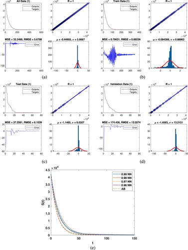
Figure 3(a) represents all data for the second class and the output we obtained through DNN. The regression is approximately 1, the mean square 0.10351 and root mean square errors 0.32172 as presented. Histogram showed the mean and variance errors while the errors are 0.0081204 and 0.32194, we observed that the data are accurate of the mentioned technique. In Figure 3(b), we present the train data for class $E_H$ results we obtained with DNN. Regression coefficient is approximately 1, the mean square 0.11826 and root mean square errors 0.34389 are obtained. Histogram plot presents mean and variance errors while these errors are 0.0008312 and 0.34438 which present the accuracy. Similarly, Figure 3(c) represents the test data for class $E_H$ and the output we obtained through DNN, regression is approximately 1, the mean square 0.11342 and root mean square errors 0.33678 we obtained. Histogram showed the mean and variance errors while these errors are $0.049176$ and $0.33541$ which present the accuracy, respectively. Similarly, Figure 3(d) represents the validation data $E_H$ and we obtained the output with DNN, the regression is approximately 1, mean square and root mean square errors are 0.024541, 0.15666 are obtained. Histogram plot presented mean and variance errors while these errors are 0.0011779 and 0.15771 which present the accuracy of the aforementioned technique. Figure 3(e) shows the dynamics of the second class along with the comparison of DNN.

Figure 3. Graphically representation of class $E_H\left(t\right)$ with deep neural network. (a) All data, (b) train data, (c) test data, (d) validation and (e) comparison of AB with NN.

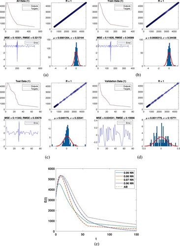
Figure 4(a) represents all data for the third class and the output we obtained through DNN. The regression is approximately 1, the mean square 0.00095856 and root mean square errors 0.030961 as presented. Histogram showed the mean and variance errors while the errors are $-0.00082128$ and 0.030981, we observed that the data are accurate of the mentioned technique. In Figure 4(b), we present the train data for class $I_H$ results we obtained with DNN. Regression coefficient is approximately 1, the mean square 0.00057007 and root mean square errors 0.023876 are obtained. Histogram plot presents mean and variance errors while these errors are 3.7678e−05 and $0.02391$ which present the accuracy. In the same fashion, Figure 4(c) shows the test data for the class $I_H$ and the obtained results are tested through DNN, regression is 1, mean square 0.0025836 and root mean square errors 0.050829 are obtained. Histogram presented the mean and variance errors while these errors are $-0.0036434$ and 0.05104 which present the accuracy, respectively. Similarly, Figure 4(d) represents the validation data $I_H$ and we obtained the output with DNN, the regression is approximately 1, mean square and root mean square errors are 0.0011517, 0.033937 are obtained. Histogram plot presented mean and variance errors while these errors are $-0.0020191$ and 0.034105 which present the accuracy of the aforementioned technique. Figure 4(e) shows the dynamics of the second class along with the comparison of DNN.

Figure 4. Graphically representation of class $I\left(t\right)$ with deep neural network. (a) All data, (b) train data, (c) test data, (d) validation and (e) comparison of AB with NN.

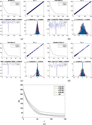
Figure 5(a) represents all data for the fourth class and the outputs are obtained through DNN. The regression is approximately 1, the mean square 4.4743e−10 and root mean square errors 2.1153e−05 as presented. Histogram showed the mean and variance errors while the errors are $-8.2368e-07$ and 2.1158e−05, we observed that the data are accurate of the mentioned technique. In Figure 5(b), we present the train data for the fourth class results we obtained with DNN. Regression coefficient is approximately 1, the mean square $4.108e-10$ and root mean square errors 2.0268e−05 are obtained. Histogram plot presents mean and variance errors while these errors are $-1.6708e-06$ and 2.0228e−05 which present the accuracy. Similarly, Figure 5(c) shows the test data for the class $R_H$ and the obtained results are tested through DNN, regression is 1, mean square $5.4498e-10$ and root mean square errors 2.3345e−05 are obtained. Histogram presented the mean and variance errors while these errors are 2.5531e−06 and 2.3361e−05 which present the accuracy, respectively. One the same fashion, Figure 5(d) represents the validation data $R_H$ and we obtained the output with DNN, the regression is approximately 1, mean square and root mean square errors are 5.2134e−10, 2.2833e−05 are obtained. Histogram plot presented mean and variance errors while these errors are $-2.3618e-07$ and 2.2985e−05 which present the accuracy of the considered technique. Figure 5(e) presents the dynamics of the $R_H$ class along with the comparison of DNN.

Figure 5. Graphically representation of class $R\left(t\right)$ with deep neural network. (a) All data, (b) train data, (c) test data, (d) validation and (e) comparison of AB with NN.

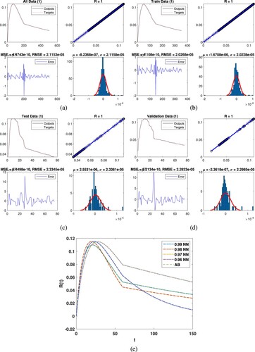
Figure 6(a) represents all data for the Fifth class and the outputs are obtained through DNN. The regression is approximately 1, the mean square 80.6655 and root mean square errors 8.9814 as presented. Histogram showed the mean and variance errors while the errors are 0.087602 and 8.9899, we observed that the data are accurate of the mentioned technique. In Figure 6(b), we present the train data for the fifth class results we obtained with DNN. Regression coefficient is approximately 1, the mean square 89.8404 and root mean square errors 9.4784 are obtained. Histogram plot presents mean and variance errors while these errors are $0.0060078$ and 9.4919 which present the accuracy. Similarly, Figure 6(c) shows the test data for the class $S_M$ and the obtained results are tested through DNN, regression is 1, mean square 60.0705 and root mean square errors 7.7505 are obtained. Histogram presented the mean and variance errors while these errors are 0.051133 and 7.8025 which present the accuracy, respectively. One the same fashion, Figure 6(d) represents the validation data $S_M$ and we obtained the output with DNN, the regression is approximately 1, mean square and root mean square errors are 58.3219, 7.6369 are obtained. Histogram plot presented mean and variance errors while these errors are 0.50593 and 7.6714 which present the accuracy of the considered technique. Figure 6(e) presents the dynamics of the $S_M$ class along with the comparison of DNN.

Figure 6. Graphically representation of class $S_m\left(t\right)$ with deep neural network. (a) All data, (b) train data, (c) test data, (d) validation and (e) comparison of AB with NN.

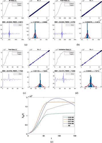
Figure 7(a) represents all data for the Fifth class and the outputs are obtained through DNN. The regression is approximately 1, the mean square 7.5654 and root mean square errors 2.7505 as presented. Histogram showed the mean and variance errors while the errors are 0.013088 and 2.7533, we observed that the data are accurate of the mentioned technique. In Figure 7(b), we present the train data for the fifth class results we obtained with DNN. Regression coefficient is approximately 1, the mean square 4.9613 and root mean square errors 2.2274 are obtained. Histogram plot presents mean and variance errors while these errors are $-0.001266$ and 2.2306 which present the accuracy. Similarly, Figure 7(c) shows the test data for the class $E_M$ and the obtained results are tested through DNN, regression is 1, mean square 5.5545 and root mean square errors 2.3568 are obtained. Histogram presented the mean and variance errors while these errors are $-0.10585$ and $2.3703$ which present the accuracy, respectively. One the same fashion, Figure 7(d) represents the validation data $E_M$ and we obtained the output with DNN, the regression is approximately 1, mean square and root mean square errors are 21.7637, 4.6652 are obtained. Histogram plot presented mean and variance errors while these errors are 0.1992 and 4.6923 which present the accuracy of the considered technique. Figure 7(e) presents the dynamics of the $E_M$ class along with the comparison of DNN.

Figure 7. Graphically representation of class $E_M\left(t\right)$ with deep neural network. (a) All data, (b) train data, (c) test data, (d) validation and (e) comparison of AB with NN.

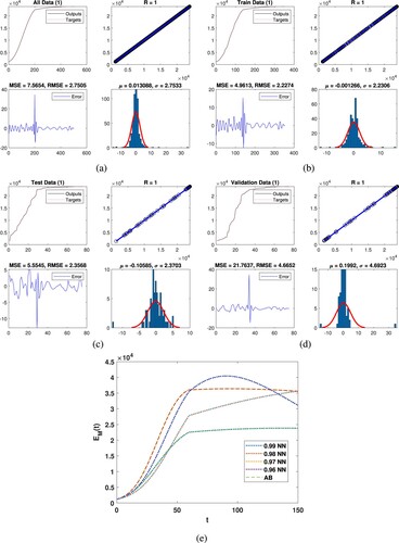
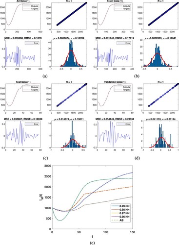
Figure 8(a) represents all data for the last class and the outputs are obtained through DNN. The regression is approximately 1, the mean square 0.035268 and root mean square errors 0.1878 as presented. Histogram showed the mean and variance errors while the errors are 0.0060674 and 0.18789, we observed that the data are accurate of the mentioned technique. In Figure 8(b), we present the train data for the last class results we obtained with DNN. Regression coefficient is approximately 1, the mean square 0.031042 and root mean square errors 0.17619 are obtained. Histogram plot presents mean and variance errors while these errors are $-0.0032003$ and 0.17641 which present the accuracy. Similarly, Figure 8(c) shows the test data for the class $I_M$ and the obtained results are tested through DNN, regression is 1, mean square $0.035867$ and root mean square errors 0.18939 are obtained. Histogram presented the mean and variance errors while these errors are 0.014374 and 0.19011 which present the accuracy, respectively. One the same fashion, Figure 8(d) represents the validation data $I_M$ and we obtained the output with DNN, the regression is approximately 1, mean square and root mean square errors are 0.054449, 0.23334 are obtained. Histogram plot presented mean and variance errors while these errors are 0.041133 and 0.23124 which present the accuracy of the considered technique. Figure 8(e) presents the dynamics of the $I_M$ class along with the comparison of DNN.

Figure 8. Graphically representation of class $I_M\left(t\right)$ with deep neural network. (a) All data, (b) train data, (c) test data, (d) validation and (e) comparison of AB with NN.

6. Conclusion

The purpose of this study was to analyse the dynamics of a dengue epidemic model using a unique piecewise derivative approach based on the Caputo and Atangana–Baleanu–Caputo operators. A piecewise derivative solution for the disease model outlined in our paper was investigated to establish its existence and uniqueness. We used the piecewise Newton polynomial approach to approximate the solution. The present paper introduces a numerical method for piecewise derivatives using both singular and non-singular kernels. We did numerical simulations of the piecewise dengue model at different fractional orders and found that piecewise operators have better dynamics than classical ones. We deployed a DNN to analyse the piecewise derivative models of dengue transmission. The architecture includes three hidden layers with 10, 100, and 10 neurons in the respective layers. The model underwent training for 1000 epochs, and the Levenberg-Marquardt Scheme was utilized to obtain the optimal set of weights, minimizing residual errors. By providing a clearer understanding of crossover behaviour dynamics, our work advances the concept of piecewise derivatives. A significant outcome of our simulations is the fact that greater vaccine efficiency resulted in a greater rate of recovery. We identified significant correspondences by analysing large quantities of numerical and graphical data, including comparisons against real data from Pakistan in 2023. Research into incorporating additional factors in this study is an exciting avenue for future research. To improve the model's predictive capabilities, these factors may include evolving vaccination strategies, weather variables, or socioeconomic variables. As a result of this holistic approach, we are likely to be able to develop more effective strategies for controlling and preventing the disease.

Acknowledgment

The authors extend their appreciation to Taif University, Saudi Arabia, for supporting this work through a project number (TU-DSPP-2024-87).

Disclosure statement

No potential conflict of interest was reported by the author(s).

Additional information

Funding

This research was funded by Taif University, Saudi Arabia, project No (TU-DSPP-2024-87).

References

- World Health Organization. Dengue control: epidemiology. Diunduh pada Vol. 25. 2018.
- Bhatt S, Gething PW, Brady OJ, et al. The global distribution and burden of dengue. Nature. 2013;496(7446):504–507. doi: 10.1038/nature12060
- Shekhar C. Deadly dengue: new vaccines promise to tackle this escalating global menace. Chem Biol. 2007;14(8):871–872. doi: 10.1016/j.chembiol.2007.08.004
- Brady OJ, Gething PW, Bhatt S, et al. Refining the global spatial limits of dengue virus transmission by evidence-based consensus. 2012. p. e1760.
- Derouich M, Abdesslam B. Dengue fever: mathematical modelling and computer simulation. Appl Math Comput. 2006;177(2):528–544.
- Esteva L, Cristobal V. Influence of vertical and mechanical transmission on the dynamics of dengue disease. Math Biosci. 2000;167(1):51–64. doi: 10.1016/S0025-5564(00)00024-9
- Qureshi S, Atangana A. Mathematical analysis of dengue fever outbreak by novel fractional operators with field data. Phys A Stat Mech Appl. 2019;526:121127. doi: 10.1016/j.physa.2019.121127
- Derouich M, Outayeb A, Twizell EH. A model of dengue fever. Biomed J Line Central. 2003;2(1):1–10.
- Esteva L, Vargas C. Analysis of a dengue disease transmission model. Math Biosci. 1998;150(2):131–151. doi: 10.1016/S0025-5564(98)10003-2
- Esteva L, Vargas C. A model for dengue disease with variable human population. J Math Biol. 1999;38(3):220–240. doi: 10.1007/s002850050147
- Hethcote HW. The mathematics of infectious diseases. SIAM Rev. 2000;42(4):599–653. doi: 10.1137/S0036144500371907
- Newton EA, Reiter P. A model of the transmission of dengue fever with an evaluation of the impact of ultra-low volume (ULV) insecticide applications on dengue epidemics. Am J Trop Med Hyg. 1992;47(6):709–720. doi: 10.4269/ajtmh.1992.47.709
- Feng Z, Velasco-Hernández JX. Competitive exclusion in a vector-host model for the dengue fever. J Math Biol. 1997;35(5):523–544. doi: 10.1007/s002850050064
- Atangana A, Baleanu D. New fractional derivatives with non-local and non-singular kernel. Therm Sci. 2016;20(2):763–769. doi: 10.2298/TSCI160111018A
- Podlubny I. Geometric and physical interpretation of fractional integration and fractional differentiation. Fract Calculus Appl Anal. 2002;5:367–386.
- Li B, Zhang T, Zhang C. Investigation of financial bubble mathematical model under fractal-fractional Caputo derivative. FRACTALS (fractals). 2023;31(05):1–13.
- Zhu X, Xia P, He Q, et al. Ensemble classifier design based on perturbation binary salp swarm algorithm for classification. CMES-Comput Model Eng Sci. 2023;135(1):653–671.
- Mahmood T, Al-Duais FS, Sun M. Dynamics of Middle East respiratory syndrome coronavirus (MERS-CoV) involving fractional derivative with Mittag-Leffler kernel. Phys A: Stat Mech Appl. 2022;606:128144. doi: 10.1016/j.physa.2022.128144
- Zhang L, Ur Rahman M, Haidong Q, et al. Fractal-fractional anthroponotic cutaneous leishmania model study in sense of Caputo derivative. Alex Eng J. 2022;61(6):4423–4433. doi: 10.1016/j.aej.2021.10.001
- Zhang L, Ur Rahman M, Ahmad S, et al. Dynamics of fractional order delay model of coronavirus disease. Aims Math. 2022;7(3):4211–4232. doi: 10.3934/math.2022234
- Mahmood T, Ur Rahman M, Arfan M, et al. Mathematical study of algae as a bio-fertilizer using fractal–fractional dynamic model. Math Comput Simul. 2023;203:207–222. doi: 10.1016/j.matcom.2022.06.028
- Xu C, Liao M, Li P, et al. Chaos control for a fractional-order jerk system via time delay feedback controller and mixed controller. Fractal Fract. 2021;5(4):257. doi: 10.3390/fractalfract5040257
- Partohaghighi M, Yusuf A, Alshomrani AS, et al. Fractional hyper-chaotic system with complex dynamics and high sensitivity: applications in engineering. Int J Mod Phys B. 2024;38(01):2450012. doi: 10.1142/S0217979224500127
- Xu C, Pang Y, Liu Z, et al. Insights into COVID-19 stochastic modelling with effects of various transmission rates: simulations with real statistical data from UK, Australia, Spain, and India. Phys Scr. 2024;99(2):025218. doi: 10.1088/1402-4896/ad186c
- Zhu X, Xia P, He Q, et al. Coke price prediction approach based on dense GRU and opposition-based learning salp swarm algorithm. Int J Bio-Inspired Comput. 2023;21(2):106–121. doi: 10.1504/IJBIC.2023.130549
- Li B, Eskandari Z, Avazzadeh Z. Dynamical behaviors of an SIR epidemic model with discrete time. Fractal Fract. 2022;6(11):659. doi: 10.3390/fractalfract6110659
- Ur Rahman M, Althobaiti A, Bilal Riaz M, et al. A theoretical and numerical study on fractional order biological models with Caputo Fabrizio derivative. Fractal Fract. 2022;6(8):446. doi: 10.3390/fractalfract6080446
- Pooseh S, Sofia Rodrigues H, Torres DFM. Fractional derivatives in dengue epidemics. In: AIP Conference Proceedings. Vol. 1389. no. 1. American Institute of Physics, 2011.
- Xu C, Liu Z, Li P, et al. Bifurcation mechanism for fractional-order three-triangle multi-delayed neural networks. Neural Process Lett. 2023;55(5):6125–6151. doi: 10.1007/s11063-022-11130-y
- Al-Sulami H, El-Shahed M, Nieto JJ, et al. On fractional order dengue epidemic model. Math Prob Eng. 2014;2014:1–6. doi: 10.1155/2014/456537
- Defterli O. Comparative analysis of fractional order dengue model with temperature effect via singular and non-singular operators. Chaos Solitons Fract. 2021;144:110654. doi: 10.1016/j.chaos.2021.110654
- Atangana A, Araz S. New concept in calculus: piecewise differential and integral operators. Chaos Solitons Fract. 2021;145:110638. doi: 10.1016/j.chaos.2020.110638
- Atangana A, Araz S. Modeling third waves of covid-19 spread with piecewise differential and integral operators: Turkey, Spain and Czechia. Results Phys. 2021;29:104694. doi: 10.1016/j.rinp.2021.104694
- Khan WA, Zarin R, Zeb A, et al. Navigating food allergy dynamics via a novel fractional mathematical model for antacid-induced allergies. J Math Tech Model. 2024;1(1):25–51.
- Shah K, Abdeljawad T, Ali A. Mathematical analysis of the Cauchy type dynamical system under piecewise equations with Caputo fractional derivative. Chaos Solitons Fract. 2022;161:112356. doi: 10.1016/j.chaos.2022.112356
- Chinnamuniyandi M, Chandran S, Changjin X. Fractional order uncertain BAM neural networks with mixed time delays: an existence and quasi-uniform stability analysis. J Intell & Fuzzy Syst Preprint. 2024;46(2):4291–4313.
- Cui Q, Xu C, Ou W, et al. Bifurcation behavior and hybrid controller design of a 2D Lotka–Volterra commensal symbiosis system accompanying delay. Mathematics. 2023;11(23):4808. doi: 10.3390/math11234808
- Qu H, Saifullah S, Khan J, et al. Dynamics of leptospirosis disease in context of piecewise classical-global and classical-fractional operators. Fractals. 2022;30(08):2240216. doi: 10.1142/S0218348X22402162
- Kilicman A. A fractional order SIR epidemic model for dengue transmission. Chaos Solitons Fract. 2018;114:55–62. doi: 10.1016/j.chaos.2018.06.031