Water–ice phase transition in frozen soils: a mesoscopic numerical study based on lattice Boltzmann method

ABSTRACT

The phenomenon of water–ice phase transition in frozen soils is the key to explaining the mechanism of frost heaving and thawing settlement disaster. However, numerical analysis of water–ice phase transitions in frozen soils at mesoscale is rarely reported. This study combines the modified Gibbs-Thomson equation and the enthalpy-based lattice Boltzmann model, and develops a mesoscale numerical method to simulate the water–ice phase transition in the local pores of saturated frozen soil during freezing and thawing process. In order to accurately simulate this process, a new η coefficient is proposed to modify the Gibbs-Thomson equation, which is unrelated to the type of soil sample and gradation characteristics. According to the particle size distribution curve, the two-dimensional random circle generation method is used to reconstruct the soil pore structure. The freezing and thawing processes are verified with the experimental data. A larger non-uniformity coefficient C_u and curvature coefficient C_c of the grain size distribution result in a lower degree of subcooling and lower residual water content of the soil during the freezing process. The new model provides an effective means to understand the water–ice phase transition in frozen soil at a mesoscopic scale.

KEYWORDS:

• Saturated frozen soils
• particle gradation
• lattice Boltzmann method
• freeze-thaw simulation
• mesoscopic scale

1. Introduction

Frost heaving and thawing settlement of the subgrade significantly affect the operational safety of transportation infrastructure in cold regions (Sheng et al. 2014, Teng et al. 2019, Chen et al. 2020, 2022). Frost heaving refers to the phenomenon of soil freezing and volume expansion at subzero temperature, generally caused by the migration and freezing of water in the soil and the growth of ice lenses in the pores. Thawing settlement is a frost disaster that volume of ice shrinks after melting, and pore water is discharged, resulting in consolidation and settlement of soil. Therefore, it is necessary to accurately and clearly understand the mechanism of water–ice phase transition in the pores of frozen soils in order to explain the phenomenon of frost heaving and thawing settlement.

The soil freezing characteristic curve (SFCC) is used to describe the relationship between unfrozen water content and the temperature during the soil freezing or thawing process, which is a basic information to reflect the water–ice phase transition in frozen soil (Wang et al. 2017, Teng et al. 2021, Zhou et al. 2021). The unfrozen water content (or ice) directly affects the amount of frost heave, permeability, and mechanical properties of the soil, and is a crucial variable for the comprehensive analysis of the freeze-thaw features. Current test methods for measuring unfrozen water content in soil include nuclear magnetic resonance (NMR), time domain reflectometry (TDR), calorimetry, etc., which are reliable and accurate (Watanabe and Wake 2009, Teng et al. 2020, Wang et al. 2022). But it is noted that the frozen soil samples used for indoor testing will freeze or thaw during sampling and transportation, and the pore structure of remoulded samples in laboratory differs from the in-situ undisturbed soil. Thus, the indoor test results of soil samples are hard to completely reflect the actual situation of the undisturbed soil. Moreover, the measured SFCC in laboratory reflects the statistical average of unfrozen water content in frozen soil, which cannot characterise the freezing state or phase transformation process in the local pores. The phase state and morphological transformation of pore water has been less understood. Currently, mesoscopic observation of the ice formation process in frozen soils is mainly based on advanced testing methods such as X-ray micro-computed tomography (CT) technology and Nuclear magnetic resonance (NMR). However, the real-time monitoring of pore characteristics of frozen soil by these methods requires extremely accurate test operation and temperature control conditions (Zhou et al. 2022). It should be noted that X-ray micro-CT technology is currently difficult to accurately distinguish between water and ice in pores (Teng et al. 2022). The NMR technology can measure the content values of the two phases of ice and water and pore size distribution during the freeze-thaw cycle (Petrov and Furó 2009, Liu et al. 2020), but it is impossible to accurately monitor the real-time evolution of the ice formation process. Therefore, there is an urgent need for appropriate methods to study and describe the pore-scale phase transition of frozen soil.

Numerical simulation can be considered an effective supplement to laboratory testing. The numerical approach not only saves cost but also allows accurate control of each variable and avoids the influence of other factors. Most numerical models of soil freezing or thawing are based on the hydrothermal coupling numerical algorithm of the macroscopic continuous equation, which establishes empirical formulas between indicators such as unfrozen water content or ice content and temperature (Wang et al. 2011, Li et al. 2018, Hu et al. 2021), and provides the results of moisture distribution, temperature and deformation in the freeze-thaw process. However, on the one hand, these numerical methods have difficulty in restoring the pore structure of the soil and lack mesoscopic study on the ice formation process of frozen soil pores. On the other hand, many empirical parameters are difficult to be given accurately, and the variation of parameters in the numerical solution process has a great influence on the calculation accuracy and robustness.

The lattice Boltzmann method (LBM) is a mesoscopic scale numerical calculation method developed in the 1980s (Song et al. 2016). It is based on discrete kinetic theory, ignores the continuous media hypothesis, does not pay attention to the motion details of individual particles, and calculates only the statistical average results of particles. It has the characteristics of both macroscopic and microscopic methods and provides new ideas for studying the mechanism of water–ice phase transition in frozen soils. The LBM has been widely used in fuel cells (Yu et al. 2018), biomedicine (Bernaschi et al. 2019), complex flow (Li et al. 2015) (Wang et al. 2019) (Yang et al. 2019), phase change energy storage materials (Jourabian et al. 2013, 2017) and other fields. But few study has been reported in the field of frozen soil.

In the limited study that applies LBM to simulate water–ice phase transition in porous media, distribution of soil temperature, water, and ice are computed and compared with the measured data. Song et al (Song et al. 2017). develop a multiphase flow model to simulate the water distribution of frozen sandy loam at different depths by incorporating the influence of soil-water potential into the fluid force. Xu et al. (Xu et al. 2018) and Zhang et al. (Zhang et al. 2018) investigated heat and mass transfer in unsaturated permafrost by introducing pre-melting theory into LBM calculations. Hu et al. (Hu et al. 2019) proposed a random growth method for porous structures that can investigate the temperature change and phase interface motion during the freezing of saturated soils. The above studies mentioned provide a way to study the phase transition process in frozen soil by using LBM, but most of them merely focus on the analysis of macro-mechanism such as the variations of temperature, water content, and ice content. The mesoscopic process of ice formation in frozen soil has been less understood. Moreover, the particle gradation characteristic, that is a feature of great importance for soil, is not considered in the previous LBM simulations.

In order to understand the mesoscopic mechanism of ice formation in frozen soils, a new numerical approach is proposed by incorporating enthalpy-based model in the LBM simulation. By reconstructing the porous structure of soil and establishing the calculation method of pore water freezing temperature based on Gibbs-Thomson equation, the freezing process of five different soil samples is successively simulated. The freeze-thaw mechanism of the soil is analysed through the SFCC curve and the water–ice phase transition process at the mesoscopic scale. The influence of soil properties including particle gradation and porosity on freeze-thaw state of soil is discussed finally.

2. Materials and methods

2.1. Reconstruction method for porous media

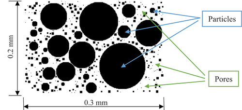
The two-dimensional random circle generation method is applied in this study. It not only meets the porosity requirements, but also controls the diameter of the random circle according with the grain grading of the original soil sample. The porous medium model is established in a rectangular computational domain. Assuming that the shape of the soil particles is circular, particles of different sizes are randomly generated to fill the original blank rectangular area until the specified porosity is reached. Based on the particle gradation of the original soil sample, the range of particle size of the porous medium and the mass fraction of each particle size can be determined. The mass fraction of sand, silt, and clay (here equivalent to the volume fraction) is selected as the control condition to reconstruct the porous structure of the soil sample. In order to control the particles from overlapping each other, when a new round particle is generated, the distance between the newly generated particle and each already generated particle is greater than the sum of their radii. For example, the particle size range of a soil sample is 1~100 μm, the porosity is 0.48, the volume fraction of sand (≥75 μm) is 40%, the silt (5 ~ 75 μm) is 50%, and the clay (≤5 μm) is 10%. In an empty 300 × 200 lattice (corresponding actual physical size: 0.3 mm × 0.2 mm), the program randomly generates coarse and fine particles with corresponding size ranges and volume fractions, and there is no overlap between the particles. The constructed porous medium is shown in Figure 1, and the black areas are particles, the white areas are pores.

Figure 1. The porous medium is generated.

The particle size distribution of the porous medium reconstructed by the model is essentially the same as that of the original soil sample so that the freeze-thaw process of the soil can be better reproduced in the subsequent simulation.

2.2. Freezing temperature of pore water in a soil

The melting temperature of pure water is T₀ = 273.15 K, while the phase transition temperature of liquid water in a soil is affected by pore size, solute concentration, interface free energy, etc., which results in a decrease in the melting point of water. According to the classical nucleation theory, the spherical ice crystals embedded in the supercooled melting body cause a change in free energy, which can be expressed by the radius of the crystal particle (Hashimoto et al. 2011),

(1) $\mathrm{\Delta }\mathit{G}=4\mathit{\pi }{r}^2{\gamma }_{\mathit{sl}}-\frac{4\pi r^3}{3}\frac{\mathrm{\Delta }T{\rho }_i{L}_a}{T_0}$(1)

Where ρ_i is the density of ice, γ_sl is the interface free energy coefficient of ice-water, and γ_sl = 0.029 J/m², ΔT=T₀-T_m, T_m is the melting temperature of pore water (K), L_a is the latent heat of the phase transition, r is the radius of the crystal particle.

The relationship curve between free energy and particle radius shows a convex shape under the same environmental conditions and reaches the maximum at the critical radius r* as shown in Figure 2. Thus, taking the partial derivative of the free energy with respect to the radius r in Equation (1)(1) $\mathrm{\Delta }\mathit{G}=4\mathit{\pi }{r}^2{\gamma }_{\mathit{sl}}-\frac{4\pi r^3}{3}\frac{\mathrm{\Delta }T{\rho }_i{L}_a}{T_0}$(1) as 0, and the relationship between the degree of supercooling and the critical radius, the Gibbs-Thomson equation, can be obtained as follows:

(2) $\mathrm{\Delta }\mathit{T}=\frac{{\mathit{\gamma }}_{\mathit{sl}}{T}_0}{{\rho }_s{L}_a}\frac{2}{r^{\ast }}$(2)

Figure 2. The variation curve of free energy with respect to the radius r.

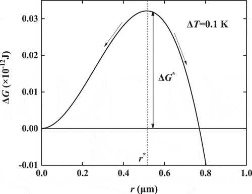
If the radius of the ice crystal in the steady state (i.e. the critical radius) is known, the ambient temperature of the current system or the supercooling degree of water can be calculated from Equation (2)(2) $\mathrm{\Delta }\mathit{T}=\frac{{\mathit{\gamma }}_{\mathit{sl}}{T}_0}{{\rho }_s{L}_a}\frac{2}{r^{\ast }}$(2) , and vice versa.

In saturated frozen soil pores, the radius of the ice-water interface arc corresponds to the critical radius r* mentioned above. In this study, a numerical calculation method of critical radius suitable for LBM is proposed: for any pore lattice in porous media, the minimum distance between this point and all solid phase nodes is taken as the value of r*, and then the phase transition temperature at the interface arc of ice-water passing through the pore lattice can be obtained by substituting r* into the Gibbs-Thomson equation.

In this study, the particle size generated by the reconstruction model for porous media is all greater than 1 μm, while the actual soil sample has a smaller minimum particle size and a smaller pore size. To meet the porosity requirements and show the complete particle shape, the constructed particles of porous medium do not overlap or touch each other. This is the difference between the two-dimensional model and the actual situation, resulting in relatively large pore size of the porous medium model and a low degree of supercooling calculated by the Gibbs-Thomson equation. Based on the above two considerations, a coefficient η smaller than 1 is introduced here to correct the critical radius r* in the Gibbs-Thomson equation:

(3) $\mathrm{\Delta T}=\frac{{\mathit{\gamma }}_{\mathit{sl}}{T}_0}{{\rho }_s{L}_a}\frac{2}{r^{\ast }\cdot \mathit{\eta }}$(3)

In order to meet the accuracy requirements of the numerical model, η is stable in a small range from 0.1 to 0.2. And the correlation between η and the type of soil sample and grading characteristics is negligible. It is recommended to choose η = 0.15 for soil.

2.3. Solid–liquid phase transition model based on enthalpy method

The enthalpy-based model of solid-liquid phase change was used to simulate the process of phase transition of water–ice during freezing (Jiaung et al. 2001), and the energy equation of phase transition of water is expressed as follows:

(4) $\frac{\mathrm{\partial T}}{\mathrm{\partial t}}=\mathit{\alpha }{\mathrm{\nabla }}^2\mathit{T}-\frac{L_a}{C_p}\frac{\mathrm{\partial }{f}_l}{\mathrm{\partial t}}$(4)

Where the second term on the right-hand side is the phase transition source term. The scalars T, t, α, L_a and C_p are temperature, time, thermal diffusivity, latent heat of phase transition, and specific heat at constant pressure, respectively. The f_l denotes the fraction of the liquid phase, f_l = 1 denotes the liquid phase region, and f_l = 0 denotes the solid phase region.

When the enthalpy value H is determined, the following can be obtained:

(5) $f_l=\left\{\begin{array}{c}0\mathit{H}<H_s\\ \frac{H-H_s}{H_l-H_s}{H}_s\le \mathit{H}\le H_l\\ 1\mathit{H}>H_l\end{array}\right.$(5)

where H_l and H_s are the enthalpy values corresponding to the initial temperature of the phase transition T_l and the final temperature of the phase transition T_s (here T_l=T_s=T_m), and the calculation formula is H_l=C_p,l T_l + L_a, H_s = C_p,s T_s. The subscripts l and s represent the liquid phase and the solid phase, respectively.

2.4. Lattice Boltzmann equation

The LBM regards fluid as a discrete collection of particles (particles can be single molecules or atoms or molecular microclusters). Each particle moves between nodes along the grid line according to certain rules, and then migrates or collides until convergence conditions or time steps are satisfied. Therefore, the lattice (discrete velocity model), the equilibrium distribution function, and the evolution equation of the particle distribution function are generally regarded as the three main components of the lattice Boltzmann model (Krüger et al. 2017).

The velocity field is discretized based on the DnQb discrete velocity model proposed by Qian (Qian et al. 1992). DnQb means that the number of discrete velocities is b in n-dimensional space. The D2Q9 model used here represents 9 discrete velocities in 2-dimensional space (including the particle that remains at the origin, i.e. the velocity is 0), as shown in Figure 3. Specifically, it can be expressed as follows:

(6) $\mathit{c}=\mathit{c}\left[\begin{array}{ccccccccc}0& 1& 0& -1& 0& 1& -1& -1& 1\\ 0& 0& 1& 0& -1& 1& 1& -1& -1\end{array}\right]$(6)

Figure 3. D2Q9 model.

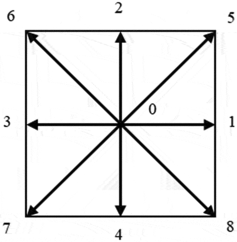
where c is the lattice speed, generally set as 1.

The enthalpy-based model for solid–liquid phase change introduces the source term of the phase transition into the evolution equation of the temperature field. Therefore, the evolution equation of the particle distribution function in the region where phase transition occurs is,

(7) $g_i(\mathit{x}+c_i\mathrm{\Delta t},\mathit{t}+\mathrm{\Delta t})=g_i(\mathit{x},\mathit{t})-\frac{1}{{\tau }_{\alpha }}\left[g_i(\mathit{x},\mathit{t})-g_i^{eq}(\mathit{x},\mathit{t})\right]-{\omega }_i\frac{L_a}{C_p}[f_l(\mathit{t}+\mathrm{\Delta t})-f_l(\mathit{t})]$(7)

where g_i (x, t) represents the temperature distribution function in the direction of discrete velocity i, at time t and position x, Δt is the time step, and the value is 1.

g_i^eq (x, t) is the local equilibrium distribution function, which can be obtained from the following equation

(8) ${g_i}^{\mathit{eq}}(\mathit{x},\mathit{t})={\omega }_i\mathit{T}(\mathit{x},\mathit{t})$(8)

The weight factor in each discrete direction is

(9) ${\omega }_i=\left\{\begin{array}{c}4/9\mathit{i}=0\\ 1/9\mathit{i}=1,2,3,4\\ 1/36\mathit{i}=5,6,7,8\end{array}\right.$(9)

For the region without phase transition, the source term in Equation (1)(1) $\mathrm{\Delta }\mathit{G}=4\mathit{\pi }{r}^2{\gamma }_{\mathit{sl}}-\frac{4\pi r^3}{3}\frac{\mathrm{\Delta }T{\rho }_i{L}_a}{T_0}$(1) does not exist. In this case, the temperature field evolution equation can be expressed as follows,

(10) $g_i(\mathit{x}+c_i\mathrm{\Delta t},\mathit{t}+\mathrm{\Delta t})=g_i(\mathit{x},\mathit{t})-\frac{1}{{\tau }_c}\left[g_i(\mathit{x},\mathit{t})-g_i^{eq}(\mathit{x},\mathit{t})\right]$(10)

The calculation formula of macro temperature is

(11) $\mathit{T}(\mathit{x},\mathit{t})=\sum _i^{\mathit{\hspace{0.17em}}}{g}_i(\mathit{x},\mathit{t})$(11)

where τ_α and τ_c are the relaxation time of the phase transition region and non-phase transition region, respectively, and the value is related to the thermal diffusivity α of this region:

(12) $\mathit{\tau }=\frac{\alpha }{c_s^2\mathrm{\Delta t}}+0.5$(12)

where c_s is the lattice sound speed.

In the water–ice transition region, the thermal diffusivity changes with the phase state of the material,

(13) $\mathit{\alpha }=f_l{\alpha }_l+\left(1-f_l\right){\alpha }_s$(13)

The liquid phase fraction f_l is obtained from Equation (2)(2) $\mathrm{\Delta }\mathit{T}=\frac{{\mathit{\gamma }}_{\mathit{sl}}{T}_0}{{\rho }_s{L}_a}\frac{2}{r^{\ast }}$(2) , and the enthalpy value is determined by modification (Zhao et al. 2017),

(14) $\mathit{H}=f_l{C}_{\mathit{p},\mathit{l}}\mathit{T}+(1-f_l)C_{\mathit{p},\mathit{s}}\mathit{T}+f_l{L}_a$(14)

In this study, the porous media reconstruction method and the enthalpy-based phase change lattice Boltzmann equation are used to simulate the freeze-thaw process of saturated soil. Since the actual size of the computational domain of the simulated soil sample is very small (all in millimetres, see Table 1), the pore fluid is assumed to be in a non-flow state, and only the variation of the temperature field in the computational domain is considered.

Table 1. Geometric parameter values of the model.

Sample number	Density (kg·m^−3)	Porosity	Grain-size distribution (%)			Particle size range (μm)	Porous media and their dimensions	Phase change process	Reference
			≤5 μm	5~75 μm	≥75 μm
Clay-1	2710	0.49	3	80	17	1～100		Thawing	Ma etal., (2017)
Sand	2630	0.4	0	0	10 0	400～1000		Thawing	Teng etal. (2020)
Silt	2760	0.42	17	69	14	1～80		Thawing
Clay-2	2710	0.41	73	27	0	1～30		Thawing
Clay-3	2215	0.41	18	82	0	1～70		Freezing	Liu etal. (2020)

Accurate implementation of the model boundary conditions is key to achieve the stability and accuracy of the program. Considering the actual environmental conditions of the frozen soil and the calculation efficiency of the model, the upper and lower boundaries of the simulation are set as constant temperature boundaries, and the left and right boundaries are periodic boundaries.

To understand the implementation process of the numerical simulation of the water–ice phase transition, the writing ideas of the LBM simulation program are summarised here:

1. According to the selected discrete velocity model (D2Q9) and the actual size of the computational domain, the corresponding grid is determined, and the discrete particles are settled on the lattice points.

2. According to the actual soil particle gradation, the porous medium structure of the soil is reconstructed, and the freezing temperature of water in each pore lattice is computed.

3. The macroscopic parameters such as temperature and liquid volume fraction are initialised, and the equilibrium distribution function of particles at each lattice point is obtained by Equation (8)(8) ${g_i}^{\mathit{eq}}(\mathit{x},\mathit{t})={\omega }_i\mathit{T}(\mathit{x},\mathit{t})$(8) , as the initial particle distribution function.

4. A collision and migration process of the evolution equation of the distribution function in a time step is performed, and the boundary conditions are treated.

5. The macroscopic temperature, liquid volume fraction, and enthalpy of the lattice are updated, and the local equilibrium distribution function is computed again.

The above calculation process of (4) and (5) are repeated, and the cycle continues until the program satisfies the convergence condition or the time step number requirement.

The convergence criterion has the following form,

(15) $\mathrm{Error}=\sqrt{\frac{\sum _x{(\mathit{T}(\mathit{x},\mathit{t}+\mathit{t})-\mathit{T}(\mathit{x},\mathit{t}))}^2}{\sum _x{(\mathit{T}(\mathit{x},\mathit{t}))}^2}}<\mathit{\epsilon },\begin{array}{cc}\mathit{\hspace{0.17em}}& \mathit{\epsilon }=1\times {10}^{-8}\end{array}$(15)

3. Result and discussion

3.1. Model validation

The SFCC of the freezing or melting process for five saturated soil samples (including clay, silt, and sand) are selected for numerical study (Ma et al. 2017, Liu et al. 2020, Jin et al. 2020). Some studies showed that the results of SFCC can vary differently for different confinements and densities even for the same soil, which is quite similar to SWCC. The adopted construction method of porous media assumes that the confinement and deformation of soil are not considered, and the characteristics of particle size distribution and pore characteristics of soil are the main concern in this study (Mu et al. 2019, Li et al. 2023). The model adopts the grid of 300 × 200. The geometric parameters of the reconstructed porous media are summarised in Table 1, including porosity, soil particle density, particle size distribution, etc. The porous media model and the phase transition process generated from the above information are included in the table as well. The reconstructed porous media model has obvious gradation characteristics, and the actual size of the computational domain varies greatly due to the limitation of the particle size range.

Regardless of whether the soil sample is actually in the freezing or melting process, the initial temperature of the whole computational domain in the simulation is set to 0°C, and then the low-temperature boundary of different degrees is applied, so that the temperature field and phase field change. Table 2 shows the values of thermal physical parameters in the simulation.

Table 2. Thermal physical parameters of materials.

Materials	Density (kg·m^−3)	Coefficient of thermal conductivity (W·m^−1·K^−1)	Specific heat capacity (J·kg^−1·K^−1)	Phase change latent heat (kJ·kg^−1)
Soil	—	1.62	850	—
Liquid water	1000	0.55	4200	336
Ice	917	2.24	2010	336

Figure 4 shows the comparison between simulated and measured SFCC values of soil samples. It can be observed that the unfrozen water content at different temperatures determined by LBM simulation is essentially consistent with the experimental values, indicating that the model and simulation program in this paper is reliable. The figure indicates the value of η for each soil sample. It can be seen that η is stable in a small range from 0.1 to 0.2, and that the correlation between η and the type of soil sample and grading characteristics is negligible. It is recommended to choose η = 0.15 for soil.

Figure 4. Freezing characteristic curves of reconstructed porous media and corresponding soil.

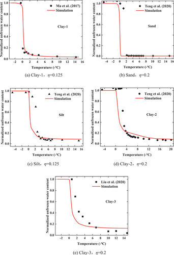
It is noted that the simulations of Clay-1, Sand, and Silt samples are relatively better than that of Clay-2 and Clay-3. Comparing the particle size distribution and porous medium model of each soil sample in Table 1, the Clay-1, Sand, and Silt samples contain a large proportion of coarse-grained soil, relatively low clay content, which has a relatively large pore size. While Clay-2 and Clay-3 contain a high percentage of clay particles (>15%), and the simulated curve obviously does not reach the supercooling degree in the experiment. Therefore, this model is more suitable for the soils with a high content of sand and silt particles. More attention should be paid on the surface characteristics when using the LBM method for clay. This model is more suitable for soils with large coarse particle content such as sand and silt, and is generally suitable for soils with large clay content and narrow particle size range.

As for the reproduction of the soil skeleton, the porous medium model considers the particles of circular shape and the particle gradation, thus the pore size solely is considered in the calculation of the freezing temperature of the pore water. However, the surface of the clay particles is negatively charged, its interaction with pore water leads to the formation of a double electric layer on the surface of clay particles (Jin etal., 2020). The freezing temperature of the bound water in the double electric layer is several degrees lower than that of the free water in the centre of the pore. At the same time, the clay particles are small and flaky with a large specific surface area, which results in a greatly increased proportion of bound water, and the pore water cannot easily freeze into ice. Therefore, the freezing process of clay is more complex and variable compared to other soil types. Using round particles to simulate the shape of clay particles may be one of the reasons why the model is not suitable for clay freezing. It needs to be discussed more comprehensively in combination with the special properties of clay particles.

3.2. Mesoscopic simulation of water–ice phase transition in frozen soil

The lattice Boltzmann model can determine the meso-evolution process of the water–ice phase transition in frozen soils, and can optionally select observation points as needed to monitor changes in pore water temperature and liquid fraction with time. This is one of the advantages of LBM compared to other simulation methods. In this section, the porous medium model corresponding to soil sample Silt in Table 1 is selected to simulate the freezing process of saturated soil, and a detailed analysis of the freezing process is performed with respect to three low-temperature boundaries and six pore points.

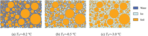
The cloud map of the volume fraction of the liquid phase in the soil at different temperatures is derived, as shown in Figure 5 (blue: f_l ≥ 0.5, light blue: f_l < 0.5). At T_w=-0.2°C, the liquid water in the centre of the macropores begins to condense into ice, but the micropores do not begin to freeze. As the temperature continues to drop, the liquid water freezes almost completely, and gradually loses continuity. Eventually, only a small amount of liquid water remains attached to the surface of the particles. This indicates that the freezing temperature of the pore water depends on the pore size and pore structure. The closer it is to the particle surface, the lower the freezing temperature will be. At this time, it is more constrained by the ice–water interface energy and particle surface energy, thus it is more difficult to freeze.

Figure 5. Phase distribution at different temperatures in silt.

In order to observe the freezing process of pore water in soil, six pore lattice points shown in Figure 6 are selected for analysis. It shows that points A, B, and C lie on the same horizontal plane, where point A has the largest pore and point B has the smallest. In the same pore, points D, E, and F are also on the same horizontal plane but are successively closer to the particle surface. The observation points are divided into two groups, and the curves of temperature change and liquid fraction change of each point at three boundary temperatures are shown in Figure 7.

Figure 6. Position of observation point in the pore (A, B, C represent the center of the selected pore, and D, E, F represent the lattice points in different positions in a pore).

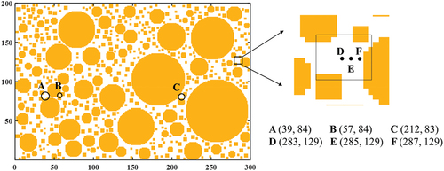
Figure 7. Change curves of temperature and liquid fraction at each observation point.

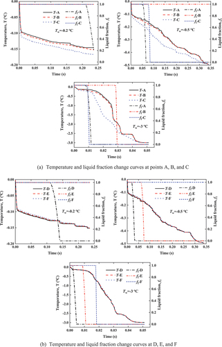
Figure 7(a) shows the temperature and liquid fraction change curves at points A, B, and C. The temperature at each point gradually decreases with time and approaches the boundary temperature eventually. Since the pores of A and B are adjacent to each other, the structure of the surrounding porous medium can be considered the same, thus the temperature change trend of the two points is similar. While point C is far away from A and B, the structure of the surrounding porous medium is completely different, and the position is closer to the lower boundary. Therefore, the shape of the temperature change curve at point C is significantly different from that of the other two points, and the overall temperature is lower. There is no significant relationship between the shape of the temperature curve of the three pore points and the size of the corresponding pores, and the three points are essentially at the same level. It indicates that the structure of the porous medium around the pores has a great influence on the temperature change.

The liquid fraction change curves of points A, B, and C show the freezing state of the lattice over time. Once the temperature of the pore water reaches the freezing point, the liquid volume fraction decreases, indicating that the pore water is frozen. At the same boundary temperature, point A freezes firstly. At different boundary temperatures, the water–ice phase transition occurs at point A when T_w=-0.2°C, followed by the phase transition at point C when T_w=-0.5°C, and finally at point B when T_w=-3°C. It indicates that a smaller pore size leads to a lower freezing point of the pore water, and a later freezing time.

Figure 7(b) shows the change of temperature and liquid fraction at points D, E, and F in a same pore. At different boundary temperatures, the temperature curves of the three points are almost in agreement, which is consistent with the above conclusion that the trend of temperature change of adjacent grid points are consistent on the same horizontal plane.

The curves for the change in the liquid fraction of points D, E, and F in Figure 7(b) are similar to those in Figure 8(a). At T_w=-0.2°C, only point D freezes. At T_w=-0.5°C, point D and point E begin to freeze in succession. At T_w=-3°C, points D, E, and F freeze sequentially. The distance between three points and particle surface is D > E > F. It indicates that the pore water closer to the particle surface has a lower freezing temperature. The energy of the particle surface has a great influence on the freezing point and the freezing state of pore water.

Figure 8. Porous medium model (calculated region: 0.3 mm×0.2 mm).

4. Parameter analysis

The proposed model has advantage to simulate the actual gradation curve for porous media. The two parameters used to describe the particle size gradation characteristics of the soil are the non-uniformity coefficient C_u and the curvature coefficient C_c. The calculation formula is as follows:

(16) $C_{\mathrm{u}}=d_{60}/d_{10},C_{\mathrm{c}}=d_{30}^2/\left(d_{60}{d}_{10}\right)$(16)

where, d₁₀, d_30, and d₆₀ represent the corresponding particle sizes when the mass fraction of soil particles smaller than a certain particle size is 10%, 30%, and 60%, respectively. The d₁₀ is the effective particle size.

In order to study the influence of soil internal structure on freeze-thaw properties in detail, the two gradation parameters C_u, C_c, and porosity n are discussed in this section. The percentage of clay particles is set to a small value, i.e. d₁₀ = 8 μm, the particle size range for all working conditions is 1 ~ 100 μm. According to the above principles, a total of 24 simulation cases are combined (excluding C_u<C_c), as shown in Table 3.

Table 3. Simulated working conditions.

Case number	n	Cu	Cc	d10/μm	d30/μm	d60/μm	T0-Tf/℃	Residual water content, Sr
1	0.45	2	1	8	11.3	16	0.1563	0.1054
2		4	1		16.0	32	0.1241	0.0787
3		6	1		19.6	48	0.1022	0.0609
4		8	1		22.6	64	0.1007	0.0622
5		10	1		25.3	80	0.0883	0.0504
6		2	2		16.0	16	0.1434	0.0920
7		4	2		22.6	32	0.1067	0.0615
8		6	2		27.7	48	0.0979	0.0560
9		8	2		32.0	64	0.0917	0.0541
10		10	2		35.8	80	0.0879	0.0510
11		4	3		27.7	32	0.1028	0.0626
12		6	3		33.9	48	0.0891	0.0489
13		8	3		39.2	64	0.0812	0.0476
14		10	3		43.8	80	0.0788	0.0457
15		4	4		32.0	32	0.0993	0.0583
16		6	4		39.2	48	0.0822	0.0503
17		8	4		45.3	64	0.0812	0.0471
18		10	4		50.6	80	0.0761	0.0419
19		6	5		43.8	48	0.0873	0.0509
20		8	5		50.6	64	0.0779	0.0466
21		10	5		56.6	80	0.0812	0.0455
22	0.55	6	2	8	27.7	48	0.0628	0.0320
23	0.65	6	2		27.7	48	0.0427	0.0197
24	0.75	6	2		27.7	48	0.0309	0.0113

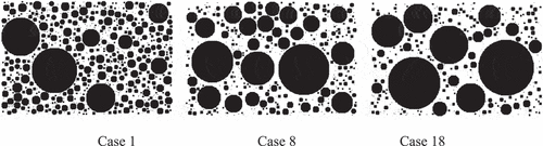
The model follows the same grid 300 × 200 and the boundary temperature T_w ranges from −25°C to 0°C. In this study, representative porous media models for working conditions 1, 8, and 18 are presented, as shown in Figure 8. At the same time, the grain-size distribution curves corresponding to the three working conditions are shown in Figure 9.

Figure 9. Soil grain-size distribution.

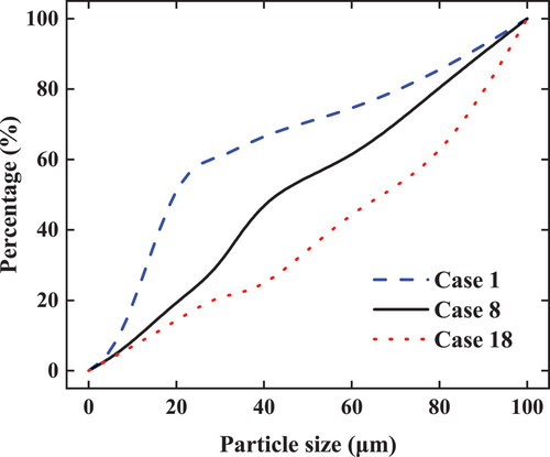
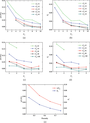
The generated structures of porous media differ significantly when the values of C_u and C_c are different as shown in Figure 8. When the porosity is same, the particle size distribution becomes more non-uniform with the increase of the non-uniformity coefficient C_u. The larger C_u and C_c are, the larger the pore size is and the smaller the pore number is. When traced to the particle size distribution curve, the curve was relatively lower with increasing C_u and C_c, indicating that the proportion of fine particles was lower, and the large pores between coarse particles are not filled with sufficient fine particles, making the pores larger. In order to facilitate the observation of the simulation results, the subcooling degree ∆T=T₀-T_f (T_f is the temperature at which soil freezing begins) and the residual water content S_r (when T_w=-25 ℃) are derived from the SFCC. The computed results are shown in Table 3.

The relationship curves between C_u, C_c, ΔT, and S_r are respectively shown in Figure 10. Figures 10(a)-10(d) show that a greater C_u value leads to a lower subcooling degree ΔT of the pore water in the soil, and a lower residual water content. As C_c increases, ∆T and S_r decrease to a certain extent, but the magnitude of the overall change is much smaller. It shows that the change curves of S_r are steeper when C_u ≤4. When C_u > 4, the curve decreases slowly, indicating that C_u has a greater effect on the frozen state of the soil than C_c and that the soil with a smaller C_u has a higher degree of supercooling. Figure 10(e) shows that as the porosity increases, ∆T and S_r decrease significantly. Because there is almost no supercooling stage in the pore water for a larger soil pore.

Figure 10. The influence of gradation parameters and porosity on the soil freezing process.

During freezing-thawing process, the water in the soil changes phase, from liquid water to solid ice or from solid ice to liquid water. When liquid water turns into ice, the ice crystals grow and expand in volume, squeezing surrounding soil particles. This will cause soil particles to displace or even break and deform, and will also change the morphology of pores. This study focuses on the water–ice phase transition during freezing-thawing process. By coupling the LBM method with discrete elements, the change of soil pore structure can be simulated. And the SFCC hysteretic phenomenon caused by multiple freeze-thaw cycles can be investigated in further.

The lattice Boltzmann method has great advantages in simulating fluid flow and phase transformation, such as being simple and efficient, and being able to deal with complex boundaries. For unsaturated soil, this method can be used to simulate the process of permeation and vapour transport. It can also be applied to the water phase transition in soils pores. The future study can be performed on the aforementioned research fields.

5. Conclusions

This study presents a new mesoscopic numerical model to simulate the water–ice phase transition in soil. The enthalpy-based lattice Boltzmann method is combined with the porous media reconstruction model in the numerical simulation. A modified Gibbs-Thomson equation is proposed to calculate the freezing temperature of pore water. Five kinds of frozen soils are used to validate the proposed model. The subsequent detailed analysis on the mesoscopic freezing stage and gradation parameters can reveal the mechanism of water–ice phase transition. The proposed model overcomes the difficulties of unknowable pore structure and ice formation process, and uncontrollable variables in traditional experimental or numerical methods. The conclusions are summarised as following:

1. The porous media reconstructed according to the gradation curve in this study can reflect the pore structure of soil samples, which is to better understand the influence of soil pore structure on the water–ice phase transition. A new parameter is used to modify the Gibbs-Thomson equation in LBM simulation. It is found that η has little relationship with the type of soil sample, and its value is recommended to be 0.1 to 0.2.

2. The calculated SFCC of five different soil samples are consistent with the experimental data, which provides validation for the proposed model. The applicability of the model is better for the melting process of soils with high content of coarse grains, such as sand and silt. The supercooling phenomenon in clay and freeze-thaw mechanism is relatively more complex, which should be paid more attention to the electronegativity of the clay surface and the effect of double electric layer.

3. The freezing level of pore water in soil is affected by pore structure, pore size, ice-water interfacial energy, and particle surface energy. The water–ice or -particle interfacial energy is inversely related to the pore size or distance to the particle surface, and the larger interfacial energy results in a lower freezing point.

4. Particle gradation has a great influence on the freezing state of soil. The increase in C_u, C_c, and porosity lead to a reduction in soil supercooling and residual water content, but the influence of C_u and porosity is more significant, indicating that adopting appropriate values for these two parameters can alleviate the influence of frost heaving.

Disclosure statement

No potential conflict of interest was reported by the author(s).

Additional information

Funding

This research was supported by the National Natural Science Foundation of China [No. 52178376], National Key R&D Program of China (No. 2022YFB2603301), Natural Science Foundation of Hunan Province [2022JJ10076].

References

- Bernaschi, M., Melchionna, S., and Succi, S. 2019. Mesoscopic simulations at the physics-chemistry-biology interface. Reviews of Modern Physics, 91 (2), 025004. doi:10.1103/RevModPhys.91.025004.
- Chen, F., et al. 2020. Progress of applied research of physical geography and living environment in China from 1949 to 2019. Acta Geographica Sinica, 75 (9), 1799–1830.
- Chen, Y., et al. 2022. Finite element analysis of heat and mass transfer in unsaturated freezing soils: formulation and verification. Computers and Geotechnics, 149, 104848. doi:10.1016/j.compgeo.2022.104848.
- Hashimoto, R., Shibuta, Y., and Suzuki, T. 2011. Estimation of solid-liquid interfacial energy from Gibbs-Thomson effect: a molecular dynamics study. ISIJ International, 51 (10), 1664–1667. doi:10.2355/isijinternational.51.1664.
- Hu, T., Wang, T., and Kogbara, R.B. 2021. A finite volume-based model for the hydrothermal behavior of soil under freeze–thaw cycles. Public Library of Science ONE, 16 (6), e0252680. doi:10.1371/journal.pone.0252680.
- Hu, Y., et al. 2019. Thermal performances of saturated porous soil during freezing process using lattice Boltzmann method. Journal of Thermal Analysis and Calorimetry, 141 (5), 1529–1541. doi:10.1007/s10973-019-09035-5.
- Jiaung, W., Ho, J., and Kuo, C. 2001. Lattice Boltzmann method for the heat conduction problem with phase change. Numerical heat transfer. Part B, Fundamentals, 39 (2), 167–187. doi:10.1080/10407790150503495.
- Jin, X., et al. 2020. Modeling the unfrozen water content of frozen soil based on the absorption effects of clay surfaces. Water Resources Research, 56 (12), e2020WR027482. doi:10.1029/2020WR027482.
- Jourabian, M., Farhadi, M., and Rabienataj Darzi, A.A. 2013. Outward melting of ice enhanced by Cu nanoparticles inside cylindrical horizontal annulus: lattice Boltzmann approach. Applied Mathematical Modelling, 37 (20–21), 8813–8825. doi:10.1016/j.apm.2013.04.003.
- Jourabian, M., Farhadi, M., and Rabienataj Darzi, A.A. 2017. Accelerated melting of PCM in a multitube annulus-type thermal storage unit using lattice Boltzmann simulation. Heat Transfer-Asian Research, 46 (8), 1499–1525. doi:10.1002/htj.21286.
- Krüger, T., et al. 2017. The lattice Boltzmann method: principles and practice. Cham: Springer International Publishing.
- Li, Q., et al. 2015. Lattice Boltzmann modeling of boiling heat transfer: the boiling curve and the effects of wettability. International Journal of Heat and Mass Transfer, 85, 787–796. doi:10.1016/j.ijheatmasstransfer.2015.01.136.
- Li, S., et al. 2018. Experimental and numerical simulations on heat-water-mechanics interaction mechanism in a freezing soil. Applied Thermal Engineering, 132, 209–220. doi:10.1016/j.applthermaleng.2017.12.061.
- Li, X., Zheng, S.F., and Wang, M., et al. 2023. The prediction of the soil freezing characteristic curve using the soil water characteristic curve. Cold Regions Science and Technology, 212, 103880. doi:10.1016/j.coldregions.2023.103880.
- Liu, J., et al. 2020. Characterizing the pore size distribution of a chloride silt soil during freeze–thaw processes via nuclear magnetic resonance relaxometry. Soil Science Society of America Journal, 84 (5), 1577–1591. doi:10.1002/saj2.20087.
- Liu, J., Yang, P., and Yang, Z.J., 2020. Electrical properties of frozen saline clay and their relationship with unfrozen water content. Cold Regions Science and Technology, 178, 103127. doi:10.1016/j.coldregions.2020.103127
- Ma, T., et al. 2017. Experimental study of effect of NaCl solution on soil freezing characteristic. Rock and Soil Mechanics, 38 (7), 1919–1925.
- Mu, Q.Y., et al. 2019. Stress effects on soil freezing characteristic curve: equipment development and experimental results. Vadose Zone Journal, 18 (1), 1–10. doi:10.2136/vzj2018.11.0199.
- Petrov, O.V. and Furó, I. 2009. NMR cryoporometry: principles, applications and potential. Progress in Nuclear Magnetic Resonance Spectroscopy, 54 (2), 97–122. doi:10.1016/j.pnmrs.2008.06.001.
- Qian, Y.H., D’Humières, D., and Lallemand, P. 1992. Lattice BGK models for navier-stokes equation. Europhysics Letters (EPL), 17 (6), 479–484. doi:10.1209/0295-5075/17/6/001.
- Sheng, D., et al. 2014. A potential new frost heave mechanism in high-speed railway embankments. Géotechnique, 64 (2), 144–154. doi:10.1680/geot.13.P.042.
- Song, W., et al. 2016. A lattice Boltzmann model for heat and mass transfer phenomena with phase transformations in unsaturated soil during freezing process. International Journal of Heat and Mass Transfer, 94, 29–38. doi:10.1016/j.ijheatmasstransfer.2015.11.008.
- Song, W., et al. 2017. Macroscopic lattice Boltzmann model for heat and moisture transfer process with phase transformation in unsaturated porous media during freezing process. Open Physics, 15 (1), 379–393. doi:10.1515/phys-2017-0042.
- Teng, J., et al. 2020. Parameterization of soil freezing characteristic curve for unsaturated soils. Cold Regions Science and Technology, 170, 102928. doi:10.1016/j.coldregions.2019.102928.
- Teng, J., et al. 2021. A mathematic model for the soil freezing characteristic curve: the roles of adsorption and capillarity. Cold Regions Science and Technology, 181, 103178. doi:10.1016/j.coldregions.2020.103178.
- Teng, J., et al. 2022. Frost heave in coarse-grained soils: experimental evidence and numerical modelling. Géotechnique, 73 (12), 1100–1111. doi:10.1680/jgeot.21.00182.
- Teng, J., et al. 2019. Experimental study of ice accumulation in unsaturated clean sand. Géotechnique, 69 (3), 251–259. doi:10.1680/jgeot.17.P.208.
- Wang, C., et al. 2022. Predicting the soil freezing characteristic from the particle size distribution based on micro‐pore space geometry. Water Resources Research, 58 (1), e2021WR030782. doi:10.1029/2021WR030782.
- Wang, C., Lai, Y., and Zhang, M., 2017. Estimating soil freezing characteristic curve based on pore-size distribution. Applied Thermal Engineering, 124, 1049–1060. doi:10.1016/j.applthermaleng.2017.06.006
- Wang, M., et al. 2019. A novel algorithm of immersed moving boundary scheme for fluid–particle interactions in DEM–LBM. Computer Methods in Applied Mechanics and Engineering, 346, 109–125. doi:10.1016/j.cma.2018.12.001.
- Wang, Z., et al. 2011. Numerical simulation of water-heat coupled movements in seasonal frozen soil. Mathematical and Computer Modelling, 54 (3–4), 970–975. doi:10.1016/j.mcm.2010.11.024.
- Watanabe, K. and Wake, T. 2009. Measurement of unfrozen water content and relative permittivity of frozen unsaturated soil using NMR and TDR. Cold Regions Science and Technology, 59 (1), 34–41. doi:10.1016/j.coldregions.2009.05.011.
- Xu, F., et al. 2018. Three phase heat and mass transfer model for unsaturated soil freezing process: part 1 - model development. Open Physics, 16 (1), 75–83. doi:10.1515/phys-2018-0014.
- Yang, G.C., et al. 2019. A comprehensive parametric study of LBM-DEM for immersed granular flows. Computers and Geotechnics, 114, 103100. doi:10.1016/j.compgeo.2019.103100.
- Yu, J., et al. 2018. Apparent contact angles of liquid water droplet breaking through a gas diffusion layer of polymer electrolyte membrane fuel cell. International Journal of Hydrogen Energy, 43 (12), 6318–6330. doi:10.1016/j.ijhydene.2018.01.168.
- Zhang, Y., et al. 2018. Three phase heat and mass transfer model for unsaturated soil freezing process: part 2 - model validation. Open Physics, 16 (1), 84–92. doi:10.1515/phys-2018-0015.
- Zhao, X., Dong, B., and Li, W., 2017. Numerical investigation on freezing process of a single freefalling droplet based on the lattice Boltzmann method. International Journal of Heat and Mass Transfer, 109, 807–811. doi:10.1016/j.ijheatmasstransfer.2017.02.050
- Zhou, J., et al. 2021. Comparison of freezing and hydration characteristics for porous media. Permafrost and Periglacial Processes, 32 (4), 702–713. doi:10.1002/ppp.2116.
- Zhou, Y., et al. 2022. Advance and review on the experimental researches of the freezing and thawing characteristics of soils. Chinese Journal of Rock Mechanics and Engineering, 41 (6), 1267–1284.