Landslide susceptibility mapping using ensemble machine learning methods: a case study in Lombardy, Northern Italy

ABSTRACT

This study compares the performance of ensemble machine learning methods stacking, blending, and soft voting for Landslide susceptibility mapping (LSM) in a highly affected Northern Italy region, Lombardy. We first created a spatial database based on open data ensuring the accessibility to relevant information for landslide-influencing factors, historical landslide records, and areas with a very low probability of landslide occurrence called ‘No Landslide Zone’, an innovative concept introduced in this study. Then, open-source software was employed for developing five Machine Learning classifiers (Bagging, Random Forests, AdaBoost, Gradient Tree Boosting, and Neural Networks) which were tested at a basin scale by implementing different combinations of training and testing schemes using three use cases. The three classifiers with the highest generalization performance (Random Forests, AdaBoost, and Neural Networks) were selected and combined by ensemble methods. The soft voting showed the highest performance among them. The best model to generate the LSM for the Lombardy region was a Neural Network model trained using data from three basins, achieving an accuracy of 0.93 in Lombardy. The LSM indicates that 37% of Lombardy is in the highest landslide susceptibility categories. Our findings highlight the importance of openness in advancing LSM not only by enhancing the reproducibility and transparency of our methodology but also by promoting knowledge-sharing within the scientific community.

KEYWORDS:

• Landslide susceptibility mapping
• machine learning
• ensemble methods
• geoprocessing
• openness
• free and open source software

1. Introduction

Landslides are geological events characterized by the downslope movement of various materials, including rocks, earth, or debris (D. Cruden 1991). These movements can be induced by several factors, such as excessive precipitation, earthquakes, human activities, or volcanic eruptions (Turner 2018). Landslides are considered one of the primary natural hazards (Yordanov and Brovelli 2021), leading to numerous casualties and significant economic losses worldwide (Budimir, Atkinson, and Lewis 2015). For this reason, numerous past and current research endeavours focus on this subject. Identifying landslide-prone areas is essential for policy-makers, scientists, engineers, and the general public to prevent catastrophic landslides. A landslide susceptibility map (LSM) can be used for this purpose, representing the spatial likelihood levels of a specific area being prone to mass movements based on environmental conditions. The foundational principles and assumptions of landslide susceptibility mapping are that future slope instabilities are more likely to occur under the same conditions that led to past and current instabilities and that the occurrence of landslides in space can be inferred through heuristic investigations, environmental information analysis, or physical modeling. Additionally, the modeling of landslide occurrence can be constructed by considering the destabilizing factors related to slope failure (Guzzetti et al. 1999).

Ado et al. (2022) have classified Machine Learning (ML) models used for landslide susceptibility mapping into four groups: conventional, hybrid, ensemble, and deep learning methods. Conventional models are standalone models that can serve as a benchmark for evaluating new models or combined with other models in hybrid or ensemble methods. The most popular conventional methods include Random Forest (RF), Support Vector Machine (SVM), Logistic Regression (LR), and Artificial Neural Network (ANN).

In a comparative study by Yordanov and Brovelli (2021), Statistical Index, LR, and RF were evaluated for their effectiveness in generating susceptibility maps. Using 11 predefined terrain variables and one precipitation variable, the study produced 79 susceptibility maps with varying ratios between training and validation datasets. The input data was refined to enhance model performance, and the results indicated that RF and LR are reliable modeling approaches. However, RF outperformed LR in most cases.

In another study, Yilmaz (2010) compared conditional probability, LR, ANNs, and SVM for generating LSM using an 11-factor spatial database. The results showed that ANN had the highest accuracy, with an AUC value of 0.846.

Hybrid techniques, which integrate feature selection and optimization methods with ML models, have demonstrated significant performance improvements compared to conventional ML methods due to their ability to address feature selection challenges (Ado et al. 2022; Y. Wang et al. 2020).

Zhao, Liu, and Xu (2021) investigated the performance of five models, including a traditional statistical Certainty Factor (CF) model, SVM, RF, and two hybrid models: CF-SVM and CF-RF. The researchers selected 10 influencing factors and used slope units as the basic mapping units. The SVM model, utilizing the Gaussian radial basis kernel function, achieved a prediction success rate of 71%, while the RF model outperformed the SVM model with a prediction success rate of 78%. The hybrid models, constructed by applying SVM or RF on the sample dataset generated by calculating the CF values of the original training samples, showed further improvement. Specifically, the CF-RF model achieved a prediction success rate of 81%, slightly outperforming the CF-SVM model with a prediction success rate of 77.5%.

Ensemble techniques combine multiple conventional ML models using different averaging or voting methods to produce more accurate predictions than conventional ML methods (Fang et al. 2021; W. Li, Fang, and Wang 2022), compensating for the limitations or biases of individual algorithms with others (Ado et al. 2022) and have already found their successful applications in the landslide susceptibility domain through homogeneous (Kadavi, Lee, and Lee 2018) or heterogeneous (Di Napoli et al. 2020) applications.

Kumar et al. (2023) explored the use of ensemble methods for regional landslide susceptibility modeling. The researchers evaluated the performance of ten individual ML models, including linear discriminant analysis, mixture discriminant analysis, Bagged Cart, Boosted Logistic Regression, K-Nearest Neighbors (KNN), Artificial Neural Network, Support Vector Machine, Random Forest, Rotation Forest, and C5.0, using different sets of landslide influencing factors ranked by an ensemble feature selection method. Subsequently, different ensemble ML models were developed and evaluated based on the suitable combination of individual ML models. The results indicated that the ensemble models of KNN+RTF, KNN+ANN, and ANN+RTF performed the best when developed using the top five landslide influencing factors.

Deep learning methods are representation-learning techniques with multiple layers of representation that can accurately predict LSM with less uncertainty (Habumugisha et al. 2022; Thi Ngo et al. 2021; Y. Wang, Fang, and Hong 2019). However, they may have low model variance and limited generalization capabilities, which can be addressed by using hybrid and ensemble setups (Kavzoglu, Teke, and Yilmaz 2021). Besides, the combination of hybrid and ensemble methods with DL models could also increase prediction accuracy (Azarafza et al. 2021; W. Li, Fang, and Wang 2022).

Overall many scholars are highlighting the fact that pure ensemble models (e.g. bagging, boosting, stacking) can lead to more accurate and reliable landslide susceptibility models (Achu et al. 2023; Kadavi, Lee, and Lee 2018; Pham et al. 2020). However, there is often lack of testing these models on their generalization capabilities, i.e. to the test the model's ability to adapt properly to new previously unseen data, drawn from the same distribution as the ones used to train the model (Baradaran and Amirkhani 2021; Ganaie et al. 2022). This is valid also in the landslide susceptibility field where usually models are trained and tested only for a specific case study.

One of the objectives of this work is to put to a test different ML techniques not only to produce reliable susceptibility maps for a specific geographic area but also to evaluate their ability to predict landslide susceptibility in other, potentially larger areas. Such implementation can potentially be more useful in practice, as can reduce the demand for big and reliable training data which in many countries is very sparse and inconsistent. To reach this objective we employed several important tasks: to implement different ensemble methods to generate landslide susceptibility maps by utilizing the most suitable base ML estimators and to evaluate the results produced by the final model. We employed three heterogeneous ensemble-learning techniques (stacking, blending, voting) for LSM by combining deep learning methods and homogeneous ensemble-learning methods. Specifically, we chose the neural network method due to its exceptionally high prediction accuracy (Ado et al. 2022), and commonly used ensemble models (Bagging, AdaBoost, Gradient Tree Boosting, and RF) for their robust predictability and efficiency (Ado et al. 2022; Sahin 2022; Y. Wang et al. 2020; Yordanov and Brovelli 2021). Initially, the approach is implemented and evaluated at a basin level in three areas (Val Tartano, Upper Valtellina, and Valchiavenna) located in Northern Lombardy. Subsequently, the methodology is extended to cover and test models' generalization ability for unseen areas, applying it to the entire region of Lombardy.

Among all model combinations in this work is proposed an innovative concept for estimating the zero-case in landslide susceptibility mapping - the No Landslide Zone (NoLsZ) for shallow landslides - based entirely on topographical and geological factors. The concept is often neglected among scholars or usually such data is fed to models in a random manner, considering everything else outside a landslide inventory as suitable to be the zero-case. However, such locations cannot be considered safe or will not fail in future, hence the need of a more structured approach. Several authors have already proposed frameworks for dealing with the issue (Marchesini et al. 2014; Sun et al. 2023) based on statistical models which naturally are bringing objective solutions. However, inherently those methods demand vast amounts of quality input data, which is not always possible uniformly everywhere, or tend to oversimplify the issue by neglecting local conditions, knowledge or landslide types. Therefore, in this work, we are motivated to propose an expert-based framework for determining areas with a negligibly low probability of shallow landslide occurrence which ultimately can be adapted for other case studies where the input information is limited.

This study aims to contribute to the landslide susceptibility mapping field through two novel methodologies. Firstly, it employs a reverse-pyramid approach in machine learning model generalization, commencing with a generic model at a basin scale and consolidating information from multiple basins to fine-tune a regional-scale predictive model for landslide susceptibility. Secondly, it introduces a concept, the No Landslide Zone, which is identified through geological criteria to highlight areas with an exceptionally low probability of landslides.

These innovations seek to enhance the existing literature by addressing the often-neglected aspects of model generalization and the inclusion of landslide-absent areas. Moreover, the work presented is entirely leveraged on openness, namely on Free and Open Source Software (FOSS), open datasets and open science (Coetzee et al. 2020), which not only supports reproducibility and transparency but further drives and promotes collaboration and knowledge-sharing not only among the scientific community but to everyone facing such geohazard challenges.

2. Materials and methods

Our work extensively utilizes the concept of openness in various ways, beginning with the use of open data as a fundamental input for both reproducible and innovative science where the overarching contribution is for datasets to be reused beyond their initial implementation (Mobasheri et al. 2020). Further, the framework was implemented in FOSS environments due to their robust maturity (Moreno-Sanchez and Brovelli 2023) and the array of benefits they offer, among them the flexibility to customize and innovate within the research domain, needs and scale (Brovelli et al. 2017). Finally, the scientific findings are openly distributed, as we are sharing the software codes and outputs that potentially can find other implementations and contribute to research in this domain.

2.1. Study area

Several small basins within the Italian Lombardy region were selected for training, testing, and evaluation of the model performance, namely Val Tartano, Upper Valtellina and Valchiavenna (Figures 1, 2). The preliminary findings from these models were later applied to a bigger area, Lombardy, to assess their generalization and the ability to produce precise landslide susceptibility maps.

Figure 1. Four areas of interest.

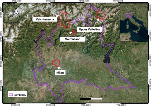
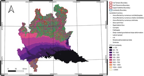
Figure 2. Areas of interest and landslide inventory.

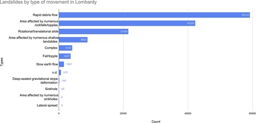
Lombardy is an administrative region that spans 23,863 km${}^2$ and is situated in the northern central part of Italy between the Alps Mountain Range and the Po River Valley. This region boasts a population of roughly 10 million individuals with a population density of 420.2 inhabits/km${}^2$ (ISTAT 2020). Lombardy is composed of 11 provinces, 1 metropolitan area (Milan), and 1523 municipalities, with Milan serving as its capital city, according to Lombardia (2020). Lombardy's varied landscape can be broadly categorized into three sections: the northern mountainous region of the Alps, the central foothills, and the southern Lombardy portion of the Padana Plain. The Lombardy region has 141,970 landslides recorded in the most recent version of the Inventory of Landslide Phenomena in Italy (Italian Landslide Inventory, IFFI) database (ISPRA 2014). Among them, the Oltrepò Pavese area and the northernmost portion of the territory have the highest density of the phenomenon (Antonielli et al. 2019). Figure 3 summarizes the frequency of various landslide types in Lombardy. Rapid debris flows, which account for 41.6% of all landslides in Lombardy, rockfalls/topples, which account for 29.7%, and rotational/translational slides, which account for 15.2%, are the main types of movement.

Figure 3. Landslide types in Lombardy region.

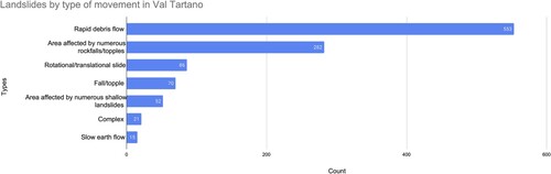
The Tartano Valley, situated in the province of Sondrio in Lombardy, Italy (46.1075${}^{\circ }$ N, 9.6791${}^{\circ }$ E), is an alpine catchment area characterized by an alpine continental climate. It covers an area of 5 km${}^2$ and has an elevation range of 250 to 2250 m a.s.l. Due to its distinctive hydrogeological characteristics, the Tartano Valley has piqued the interest of numerous authors (Colombera and Bersezio 2011; Longoni et al. 2016). This valley has experienced several flood events, including a catastrophic one in 1987, caused by heavy rains and snowmelt that triggered flooding, mudslides, and mass movements, leading to 20 fatalities and significant damage to river bank protection. Additionally, the landslide inventory of the Italian Institute for Environmental Protection and Research (ISPRA) (ISPRA 2014) documents over 1000 landslide events in this basin. The most frequent type of landslide (about 51.2%) in Val Tartano is rapid debris flow, as displayed in Figure 4.

Figure 4. Landslide types in Tartano Valley.

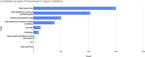
The Upper Valtellina Valley, located close to the border of Trentino-Alto Adige, comprises the second region of interest. Spanning an area of 295 km${}^2$ and an elevation range of 900 to 3800 m a.s.l., this area experiences frequent instabilities due to decompression caused by melting glaciers. According to ISPRA (2014), over 3600 individual landslide events have been recorded in this region, and the main category of landslides is rapid debris flow which is about 41% of the total landslides (Figure 5).

Figure 5. Landslide types in Upper Valtellina.

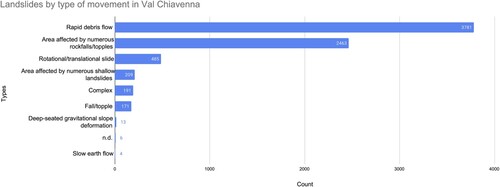
The Chiavenna Valley, located in the province of Sondrio, is an alpine valley covering an area of 578 km${}^2$, comprising two orthogonal branches: the San Giacomo Valley, oriented north to south, and the Bregaglia Valley, oriented east to west. These two branches converge near Chiavenna, forming a broader main valley running from north to south. Within these valleys, cliffs, cirques, and narrow tributary valleys can be found. The Mera River flows southward through the Bregaglia Valley and Valchiavenna before merging into Lake Como. The complex geography of the valley has attracted the interest of several scholars (Bajni et al. 2021; Tantardini, Stevenazzi, and Apuani 2022). Figure 6 illustrates the types of landslides that occurred in Valchiavenna, with data from the landslide inventory of ISPRA (2014), where more than 7000 individual landslide events have been recorded and fast debris flow was the main type of landslides, accounting for 51.6% of the total number of landslides.

Figure 6. Landslide types in Valchiavenna.

2.2. Data

2.2.1. Landslide inventory

A relatively recently updated (2017) version of Italian Landslide Inventory (IFFI) established by ISPRA, which is the official national database on landslides with a scale of 1:10,000, online since 2005, was utilized in this study (Trigila, Iadanza, and Spizzichino 2010). The IFFI incorporates a geospatial dataset containing polygonal and linear landslides of different types (Trigila, Iadanza, and Spizzichino 2010) which was constructed by historical and archival data, alongside manual aerial photo interpretation, on-site field surveys, and comprehensive mapping efforts. Each landslide in the database is accompanied by a detailed datasheet outlining its location, movement type (classification proposed by D. M. Cruden and Varnes 1996 with some modifications), and activity status. This study focuses only on susceptibility mapping of shallow types of landslides, i.e. debris flows and slides. Due to the mapped scale, linear landslides were mapped as linear features as their length is much greater than the width, thereby posing difficulties in the subsequent processing stage. To address this concern, it was recognized that all linear landslides fall under the ‘debris flow’ classification, that typically take place in narrow valleys and channels. As per the solution proposed by Yordanov and Brovelli (2021), the width of linear landslides was estimated to be approximately 10 meters.

2.2.2. No landslide zone

As a previous study suggests, when analyzing high landslide density areas, defining the low-risk zone as the entire area outside the landslide inventory can produce poor models (Yordanov and Brovelli 2021). In fact, due to the high landslide density, the landslide features end up covering the whole range of values of the terrain variables, making it hard to distinguish areas that are susceptible to mass movements from areas that are not. To avoid this issue, it was decided to define the so-called ‘No Landslide Zone’ with a geological criterion, therefore enhancing the control over the areas that are by hypothesis not susceptible to landslides. The criterion choice was improved after a few failed attempts, which led to unsatisfactory results. The final version considers as variables the terrain slope and the Intact Uniaxial Compressive Strength (IUCS), an index dependent on the lithology that describes the maximum stress that a material can take before failing. In practical terms and upon consultation with geologists, the lithology of our case study's terrain was linked with an estimate of the IUCS value (Table 1). The formula for the computation of the NoLsZ can be found in Equation (1(1) $(\mathrm{slope}<5^{\circ })\vee \left[\right(5^{\circ }<\mathrm{slope}<{20}^{\circ }\vee \mathrm{slope}>{70}^{\circ })\wedge (\mathrm{IUCS}>100\mathrm{MPa}\left)\right]$(1) ). In broad terms, areas with very low inclination ($<5^{\circ }$) were included with no other constraint. On the other hand, terrains with low ($5^{\circ }--{20}^{\circ }$) or very high ($>{70}^{\circ }$) inclination required a resistant terrain (with an IUCS of at least 100 MPa) to be included. (1) $(\mathrm{slope}<5^{\circ })\vee \left[\right(5^{\circ }<\mathrm{slope}<{20}^{\circ }\vee \mathrm{slope}>{70}^{\circ })\wedge (\mathrm{IUCS}>100\mathrm{MPa}\left)\right]$(1)

Table 1. Intact uniaxial compressive strength classification.

Field estimate of Strength	Examples	Strength [MPa]
Specimen can only be chipped with a geological hammer	Fresh basalt, chert, diabase, gneiss, granite, quarzite	$>250$
Specimen requires many blows of a geological hammer to fracture it	Amphibiolite, sandstone, basalt, gabbro, gneiss, granodiorite, limestone, marble, tuff	100–250
Specimen requires more than one blow of a geological hammer to fracture it	Limestone, marble, phyllite, sandstone, schist, shale	50–100
Cannot be scraped or peeled with a pocket knife, specimen can be fractured with a single blow from a geological hammer	Laystone, coal, concrete, schist, shale, siltstone	25–50
Can be peeled with a pocket knife with difficulty, shallow indentation made by firm blow with point of a geological hammer	Chalk, rocksalt, potash	5–25
Crumbles under firm blows with point of a geological hammer, can be peeled with a pocket knife	Highly weathered or altered rock	1–5
Indented by thumbnail	Stiff fault gouge	0.25–1

2.2.3. Landslide influencing factors (LIFs)

In this study, 12 factors were selected according to the previous studies in a similar area (Yordanov and Brovelli 2021):

• Elevation (DTM);

• Eastness;

• Northness;

• Plan curvature;

• Profile curvature;

• Topographic Wetness Index (TWI);

• NDVI;

• Distance from roads;

• Distance from rivers;

• Distance from faults;

• Land use;

• Precipitation.

All the data (Table 2) used in this study is entirely free and open source, available on the web and distributed by Geoportale della Regione Lombardia under IODL 2.0 license, Istituto Superiore per la Protezione e la Ricerca Ambientale IdroGEO under CC BY-SA 4.0 license and Agenzia Regionale per la Protezione Ambientale ARPA Lombardia under CC BY 4.0 license.

Table 2. Data type and source.

Data	Type	Source
Land use	Vector data (Polygon)	GeoPortale Lombardia
Area of Interest	Vector data (Polygon)	Custom made
Fault lines	Vector data (Line)	GeoPortale Lombardia
Geology	Vector data (Polygon)	GeoPortale Lombardia
Streams wet area	Vector data (Polygon)	GeoPortale Lombardia
Road elements	Vector data (Polygon)	GeoPortale Lombardia
Elevation (DTM)	Raster data (Resolution: 5mx5m)	GeoPortale Lombardia
Precipitation	Raster data (Resolution: 1500mx1500m)	ARPA Lombardia

Slope, eastness, northness, profile curvature, plan curvature, and TWI were calculated utilizing the DTM. The NDVI was computed through Google Earth Engine, utilizing Sentinel-2 satellite imagery spanning the entire year of 2020. Additionally, the factors ‘distance from roads’, ‘distance from rivers’ and ‘distance from faults’ were derived individually from the data sources ‘road elements’, ‘streams wet area’ and ‘fault lines’.

Slope and lithology layers were excluded from the factors considered because they were exploited for the definition of NoLsZ, and their further inclusion can produce biased outputs.

The available precipitation data obtained from the local environmental agency is with a very coarse resolution (1500 m/pix) and as such its implementation on a basin scale was not useful as the precipitation variation at each case study basin was very low. Therefore, the precipitation information was included as an additional variable only as a last iteration to the best-performing model for the Lombardy region. Two-fold modeling was included for the precipitation -- on one hand, the average interpolated hourly precipitation for the year 2020 was included and on the other, only the 90th percentile which represents exceptional intensive events for the same year was added.

In this study, the pixel size, equivalent to the DTM resolution ($5\times 5$ m), was employed as the mapping unit since most terrain variables are calculated from DTM, and this scale is sufficient for vector factors such as road and river networks. Additionally, this scale is appropriate for polygonal landslides and approximated linear landslides, taking into account the scale of the landslide inventory (1:10,000) (Yordanov and Brovelli 2021). Given that the NDVI was calculated from Sentinel-2 satellite imagery with a resolution of 10x10m, the resulting NDVI would be resampled to $5\times 5$ m using the nearest neighbor method.

2.3. Methods

2.3.1. Workflow

The overall workflow of the performed processing for the current study is represented in Figure 7. To select the most suitable base classifiers, five models (Bagging, Random Forests, AdaBoost, Gradient Tree Boosting, and Neural Network) are trained and evaluated on the case study regions using the Python package scikit-learn. Several scenarios are based on the different training datasets and test sets used for this process (Table 3).

Figure 7. Processing workflow.

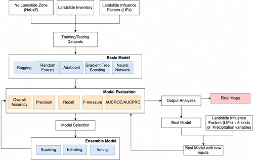
Table 3. Source of training dataset and testing dataset.

Case	Code	Trained using data sampled from	Tested on data sampled from
Val Tartano	VT	Val Tartano	Val Tartano
Upper Valtellina	UV	Upper Valtellina	Upper Valtellina
Valchiavenna Case 1	VCC	Val Tartano, Upper Valtellina	Valchiavenna
Valchiavenna Case 1	VCC2	Val Tartano, Upper Valtellina, Valchiavenna	Valchiavenna
Valchiavenna Case 1	VCC3	Valchiavenna	Valchiavenna
Northern Lombardy + Val Tartano	LC1 + VT	Val Tartano	Northern Lombardy
Northern Lombardy + Upper Valtellina	LC1 + UV	Upper Valtellina	Northern Lombardy
Northern Lombardy + Val Tartano, Upper Valtellina	LC1 + VT + UV	Val Tartano, Upper Valtellina	Northern Lombardy
Northern Lombardy + Valchiavenna Case 2	LC1 + VCC2	Val Tartano, Upper Valtellina, Valchiavenna	Northern Lombardy
Northern Lombardy + Valchiavenna Case 3	LC1 + VCC3	Valchiavenna	Northern Lombardy
Lombardy + Val Tartano	LC2 + VT	Val Tartano	Lombardy
Lombardy + Upper Valtellina	LC2 + UV	Upper Valtellina	Lombardy
Lombardy + Val Tartano, Upper Valtellina	LC1 + VT + UV	Val Tartano, Upper Valtellina	Lombardy
Lombardy + Valchiavenna Case 2	LC2 + VCC2	Val Tartano, Upper Valtellina, Valchiavenna	Lombardy
Lombardy + Valchiavenna Case 3	LC2 + VCC3	Valchiavenna	Lombardy

To achieve one of the general objectives of this work, i.e. to test also the models by transfer learning was applied a reverse-pyramid approach. Meaning, we have started the implementation with generic models on a basin scale to assess the base models' performance and applicability, followed by a consolidation of information from multiple basins to develop models able to model the susceptibility levels on a regional level. Such a consolidation of information is important when transferring to a larger scale as it introduces synthesizing data and insights from different sources with more meaningful patterns leading to more accurate and refined predictive models. Such implementation allows further expansion of the input information and the inclusion of factors that on a basin scale do not bring added value (e.g. in our case the precipitation information).

• Val Tartano (VT): train and evaluate five models using the dataset sampled from Val Tartano;

• Upper Valtellina (UV): train and evaluate five models using the dataset sampled from Upper Valtellina;

• Valchiavenna

  • – Case 1 (VCC1): train five models using the dataset sampled from Val Tartano and Upper Valtellina, and evaluate each model using the dataset sampled from Valchiavenna;

  • – Case 2 (VCC2): train five models using the dataset sampled from Val Tartano, Upper Valtellina and Valchiavenna, and evaluate each model using the dataset sampled from Valchiavenna;

  • – Case 3 (VCC3): train and evaluate five models using the dataset sampled from Valchiavenna;

• Lombardy

  • – Case 1 (LC1): evaluate each model trained in the above five cases (Val Tartano, Upper Valtellina, Valchiavenna Case 1, Valchiavenna Case 2, Valchiavenna Case 3) using the dataset sampled from the northern part of Lombardy excluding Val Tartano, Upper Valtellina, and Valchiavenna. The mountainous area of Northern Lombardy was chosen as the evaluation region because Lombardy as a whole contains a high percentage of flat areas (NoLsZ about 49.48%), which biases the evaluation for class 1 (i.e. LS). Therefore, the Po Plain portion of Lombardy is omitted, leaving only the northern alpine region, which actually hosts the majority of recorded landslide events. The total area of the 71,925 recorded landslides in Lombardy accounts for 11.88% of its total area. At the same time, 99.98% of the total number of IFFI landslides are concentrated in the northern alpine region.

  • – Case 2 (LC2): evaluate each model trained in the above five cases (Val Tartano, Upper Valtellina, Valchiavenna Case 1, Valchiavenna Case 2, Valchiavenna Case 3) using the dataset sampled from the whole Lombardy region excluding Val Tartano, Upper Valtellina, and Valchiavenna.

In this study, the primary software and tools employed include Python and QGIS. Python is an open-source programming language extensively utilized across the entire research workflow, encompassing tasks such as data preparation, model training, evaluation, and LSM generation, using the scikit-learn machine learning library, along with Python's numerical science libraries NumPy and SciPy. QGIS, a free and open-source software, is integrated with Python to preprocess the initial data and visualize and explore the data throughout every stage of the analysis.

2.3.2. Training data preparation

The datasets used in this study comprise two types of data: one is from the historical landslides inventory (designated as the ‘Landslide zone’), and is assigned a value of 1; the other is from regions where the likelihood of landslide incidence is almost negligible (termed as the NoLsZ), and is assigned a value of 0. Table 4 provides the number of sample points allocated for each area, taking into account the study area's size. Notably, no training dataset was needed for Lombardy since no model was trained for the entire region. The ratio between Landslide zone and NoLsZ in the training/testing sets was always kept 1:1. The distribution of data between training and testing sets followed an 80/20 ratio, a standard scheme for separating the available dataset in two partitions – one used for actually training the model and the other part that had never been ‘seen’ by the model, is used for its evaluation. However, it is worth noting that in the Valchiavenna case, this ratio varied slightly due to the testing dataset in this area being utilized not only for the model trained specifically with the Valchiavenna training dataset (VCC3) but also in other cases (VCC1 and VCC2).

Table 4. Number of sampled points for each studied area, including both points for NoLsZ (class 0) and LSZ (class 1).

Zone	Number of sample points for training	Number of sample points for testing
Val Tartano	15,560	3,904
Upper Valtellina	79,148	19,793
Valchiavenna	80,000	25,000
Lombardy	–	400,000

2.3.3. Machine learning methods

Below will be briefly introduced to all of the machine learning models used in the current study.

Bootstrap aggregating (Bagging), also known as bagging, is a machine learning algorithm that improves the accuracy and stability of machine learning algorithms used in statistical classification and regression, as well as reducing variance and avoiding overfitting. Various subsets of the training data are randomly drawn with replacements from the entire training dataset, and each bootstrap sample is used to train a different classifier with the same type. The individual classifiers are then combined by taking a simple majority vote on their decisions to produce the final prediction (Breiman 1996). The implemented method in this study only has one hyperparameter to tune, i.e. the number of base estimators in the ensemble.

Random Forests (RF) is one of the most widely used machine learning algorithms for classification and regression, which creates multiple decision trees by introducing randomness at the training phase. By a majority vote, these decision trees are used to determine the final prediction result. The implemented RF method involves a tunning hyperparameter, that is the number of decision trees to be generated in the forest.

AdaBoost, which stands for adaptive boosting, is a statistical classification meta-algorithm introduced by Yoav Freund and Robert Schapire in 1995 (Freund and Schapire 1997). The principle of AdaBoost is to fit a sequence of weak learners which are only slightly better than random prediction such that subsequent weak learners are tweaked in favor of those instances misclassified by previous classifiers. Using a weighted majority vote or sum, all the weak learners' predictions are combined to produce the final prediction. The implemented method includes two hyperparameters: the learning rate and the maximum number of estimators at which boosting is terminated.

Gradient Tree Boosting or Gradient Boosted Decision Trees (GBDT) is a generalization of boosting to arbitrary differentiable loss functions (J. H. Friedman 2001), which can be used for both regression and classification problems. In this algorithm, the model is built in a forward stage-wise fashion and it allows for the optimization of arbitrary differentiable loss functions. In each stage, multiple regression trees are fit on the negative gradient of the loss function. The implemented method has two hyperparameters to tune, i.e. the learning rate and the number of boosting states to perform.

Neural network (NN) algorithms can be used for both classification and regression problems. The process starts with the perceptron which takes inputs, multiplies them by some weights, and passes them to an activation function to produce an output. By adding layers of these perceptrons together, a neural network is created, which is known as a multi-layer perceptron (MLP) model. The NN consists of three layers types -- the input, hidden, and output layers. The input layer receives data directly, whereas the output layer creates the desired output. The layers in between are known as hidden layers, where the intermediate computation takes place. The NN implemented in this research comprises four hyperparameters: size, activation function for the hidden layer, and the initial learning rate. ‘size’ refers to the number of nodes in the hidden layer.

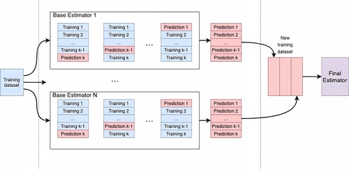
Ensemble Stacking is a method for combining estimators to reduce their biases (Wolpert 1992). The flowchart of the stacking ensemble model is shown in Figure 8. It contains the following steps: (1) using the training dataset to train different base estimators through k-fold cross-validation; (2) the predictions of each estimator are stacked together and used as input to a final estimator; (3) training the final estimator through cross-validation. The Logistic Regression model served as the meta-classifier for the final susceptibility prediction, and the method implemented in this study does not involve tuning hyperparameters.

Figure 8. Flowchart of ensemble stacking.

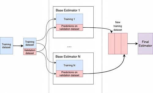
Ensemble Blending is a variation of the stacking ensemble originally introduced in the Netflix competition (Töscher, Jahrer, and Bell 2009). The flowchart of the blending ensemble model is shown in Figure 9. It consists of the following steps: (1) split the training dataset into new training and validation datasets by a hold-out method; (2) train all the base estimators using the new training dataset and make predictions of the validation dataset to form training dataset used as input to a final estimator; (3) train the final estimator. The Logistic Regression model was used as the meta-classifier for final susceptibility prediction and the implemented method in this study has no tuning hyperparameters.

Figure 9. Flowchart of ensemble blending.

Ensemble Voting's principle is to combine different estimators and use a majority vote (hard voting) or the average predicted probabilities (soft voting) to generate the final prediction. In the study, soft voting (SV) is adopted which makes the prediction based on the maximum value of the weighted average of predicted probabilities. The implemented method does not have any hyperparameter to tune.

In this study, all methodologies were performed using the Scikit-Learn library (Pedregosa et al. 2011) in Python, with the fine-tuning of hyperparameters achieved through the ‘Grid-SearchCV’ module in Scikit-Learn.

2.3.4. Model evaluation metrics

A confusion matrix constructed by using a testing dataset is used to evaluate the model. From the confusion matrix, the following statistical indexes were derived and used for evaluation. (2) $\mathrm{Overall}\mathrm{Accuracy}\left(\mathrm{OA}\right)=\frac{\mathrm{TP}+\mathrm{TN}}{\mathrm{TP}+\mathrm{FP}+\mathrm{TN}+\mathrm{FP}}$(2) (3) $\mathrm{Precision}=\frac{\mathrm{TP}}{\mathrm{TP}+\mathrm{FP}}$(3) (4) $\mathrm{Recall}\left(\mathrm{Sensitivity}\right)=\frac{\mathrm{TP}}{\mathrm{TP}+\mathrm{FN}}{F}_1=\frac{2\ast \mathrm{Precision}\ast \mathrm{Recall}}{\mathrm{Precision}+\mathrm{Recall}}$(4) (5) $\mathrm{FPR}=\frac{\mathrm{FP}}{\mathrm{FP}+\mathrm{TN}}$(5) (6) $\mathrm{TNR}\left(\mathrm{Specificity}\right)=\frac{\mathrm{TN}}{\mathrm{TN}+\mathrm{FP}}$(6) where True Positive (TP) and False Positive (FP) are the number of samples correctly classified and misclassified as positive, respectively, while True Negative (TN) and False Negative (FN) are the number of samples correctly classified and misclassified as negative, respectively.

Besides, Receiver Operating Characteristic (ROC) curve (Bradley 1997) and Precision-Recall Curve (PRC) are also adopted as comparative metrics, where PRC is also sensitive to an eventual imbalance in data classes (Yordanov and Brovelli 2020). The ROC curve is constructed by plotting the true positive rate (TPR, also known as recall) against the false positive rate (FPR) at various thresholds. The area under the curve of ROC (AUC-ROC) is widely adopted for model comparison and considered the best evaluation metric (Ado et al. 2022). This value varies between 0 and 1, where 0.5 indicates the classifier is uninformative whilst 1 represents perfect performance. PRC is created by plotting the precision against the recall at various threshold settings. Similar to the ROC curve, the area under the PRC (AUC-PRC) can be computed to indicate the model performance with a random classifier that has a value close to 0.5.

In addition to the straightforward 0.5 fixed threshold, two types of optimum thresholds are considered. One is the optimum ROC-based threshold providing the best trade-off between sensitivity and specificity which can be determined by maximizing Youden's J-statistic (Youden 1950), a statistic that captures the performance of dichotomous diagnostic tests and can be calculated using the formula below (7) $J=\mathrm{sensitivity}+\mathrm{specificity}-1$(7) Another optimum PRC-based threshold considering both precision and recall can be determined by maximizing the $F_1$ score since the $F_1$ score is the harmonic mean of precision and recall and $F_1$ score value of 1.0 indicates perfect precision and recall ($\mathrm{FP}=0$ and $\mathrm{FN}=0$).

3. Results

In the current section are presented the results from all of the implemented analyzes, starting from the NoLsZ hypothesis testing, evaluating the performance of the base and ensemble machine learning models, the inclusion of precipitation as an influencing factor, and finally presenting the landslide susceptibility map of Lombardy region. All of the derived results are available for downloading from Zenodo (Xu et al. 2023; Xu, Yordanov, and Brovelli 2023a, 2023b, 2023c, 2023d).

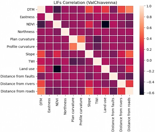
The LIFs for each study area, as utilized in this study, are presented in the Appendix 3. Correspondingly, Figures 10, 11, 12 also illustrate the correlation analysis between these factors. Notably, all correlation coefficients fall below 0.6, signifying a weak relationship between each pair of factors.

Figure 10. LIFs correlation for Val Tartano.

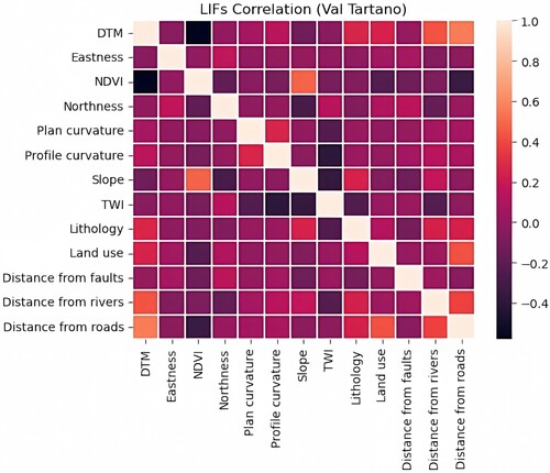
Figure 11. LIFs correlation for Upper Valtellina.

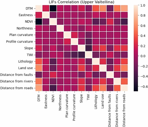
Figure 12. LIFs correlation for ValChiavenna.

3.1. No landslide zone

The areas with very low to negligible probability of landslide occurrence under the previously defined hypothesis of NoLsZ were computed for the three basins and Lombardy region at large. In order to estimate the hypothesis eligibility the products of the NoLsZ were compared with the existing IFFI landslide inventory. Naturally, some disagreements can occur between the mass movement records and presumable stable areas, mainly due to the mapped landslide extents and not always precise delineation of the failure location and mass runoff. The error estimate for the Upper Valtellina region has an overlapping ratio of 1.7% between the NoLsZ and the Landslide zone, while Val Tartano has a ratio of 0.5%. Similarly, Valchiavenna has a ratio of 1.8% and Lombardy has a ratio of 2.3%. These overlap areas can be considered negligible and support the NoLsZ hypothesis. Upon the elimination of the errors from the NoLsZ, the derived zones were used for the null case in the further ML models. The final estimate of NoLsZ covers an area of 13,325 km${}^2$ or 56% of the overall Lombardy area.

3.2. Performance evaluation

3.2.1. Base classifiers

Effective selection of optimal base classifiers plays a critical role in achieving successful landslide susceptibility mapping using ensemble models. To assess the performance of each base classifier, we evaluated its effectiveness when applied to different study areas. Figure 13 depicts the calibration curves for all base models in Val Tartano, with the average predicted probability for each bin on the x-axis and the fraction of positive classes in each bin on the y-axis.

Figure 13. Calibration plots of base classifiers for Val Tartano.

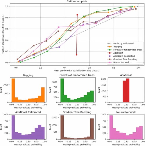
In all cases, Bagging, RF, Gradient Tree Boosting, and NN classifiers exhibit well-calibrated predictions. This is evidenced by the proximity of all curves generated by these models to the diagonal line, which represents perfect calibration.

In contrast to other classifiers, AdaBoost exhibits a distinct pattern where the probability histograms display peaks at around 0.4 and 0.6 probabilities, while probabilities at other levels are relatively infrequent. A possible explanation for this phenomenon is that AdaBoost can be viewed as an additive logistic regression model, in which the predictions made by boosting attempt to fit a logit of the true probabilities instead of the actual probabilities themselves (J. Friedman, Hastie, and Tibshirani 2000). As a result, it is essential to calibrate this classifier in all cases. The calibration result of AdaBoost with sigmoid regression is also illustrated in Figure 13 and shows well-calibrated behavior.

Different evaluation statistics (e.g. OA, precision, recall, and F-measure) of ML base classifiers for the case studies were calculated (see Tables 5, 6, 7, and Figure 14). Compared to the uncalibrated version, the calibrated version of AdaBoost does not significantly alter prediction accuracy measures. Therefore, the calibrated AdaBoost will be used in place of the uncalibrated AdaBoost in subsequent analyzes.

Figure 14. Evaluation indices of base classifiers for different cases.

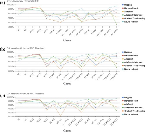
Table 5. Overall accuracy (threshold = 0.5) of base classifiers for different cases.

Cases	Bagging	Random Forest	AdaBoost	AdaBoost Calibrated	Gradient Tree Boosting	Neural Network
VT	90.37%	91.44%	85.48%	85.60%	89.75%	78.25%
UV	90.70%	90.89%	88.32%	88.57%	89.54%	87.12%
VCC2	94.36%	94.34%	89.61%	89.64%	93.30%	89.01%
VCC3	94.76%	95.07%	92.22%	92.25%	94.76%	86.33%
VCC1	69.28%	75.16%	78.82%	78.81%	68.41%	79.66%
LC1 + VT	80.08%	76.58%	78.68%	79.05%	64.77%	71.99%
LC1 + UV	66.92%	76.34%	75.89%	77.18%	60.55%	75.91%
LC1 + VT + UV	71.66%	77.33%	84.93%	85.04%	70.07%	75.69%
LC1 + VCC2	77.11%	81.31%	80.86%	80.87%	73.34%	85.83%
LC1 + VCC3	68.10%	67.97%	60.99%	60.62%	61.68%	90.82%
LC2 + VT	83.03%	78.47%	80.34%	80.68%	65.89%	73.24%
LC2 + UV	66.00%	78.57%	80.99%	81.70%	66.83%	77.38%
LC2 + VT + UV	74.17%	79.53%	87.07%	87.20%	71.00%	77.09%
LC2 + VCC2	82.84%	89.67%	87.48%	88.05%	80.91%	93.10%
LC2 + VCC3	89.91%	81.77%	55.90%	55.56%	72.13%	97.01%

Table 6. Overall accuracy based on optimum ROC-based thresholds of base classifiers for different cases.

Cases	Bagging		Random Forest		AdaBoost		AdaBoost Calibrated		Gradient Tree Boosting		Neural Network
	OA	Threshold	OA	Threshold	OA	Threshold	OA	Threshold	OA	Threshold	OA	Threshold
VT	91.78%	0.4100	92.90%	0.3700	85.66%	0.4998	85.86%	0.4749	90.24%	0.3343	82.25%	0.2637
UV	90.93%	0.4167	91.36%	0.3900	88.53%	0.5001	88.57%	0.5031	89.66%	0.4525	87.27%	0.4637
VCC2	94.40%	0.5500	94.36%	0.5200	89.81%	0.5002	89.78%	0.5282	93.42%	0.5596	89.05%	0.4861
VCC3	94.76%	0.5500	95.15%	0.5400	92.29%	0.5001	92.35%	0.5151	94.82%	0.5257	86.36%	0.4574
VCC1	70.50%	0.5300	75.17%	0.5000	79.60%	0.4990	79.58%	0.2818	69.23%	0.5899	86.00%	0.0018
LC1 + VT	83.06%	0.4300	80.44%	0.4250	91.14%	0.4899	90.91%	0.0030	80.03%	0.0005	89.95%	0.0073
LC1 + UV	71.34%	0.3725	85.33%	0.3600	75.90%	0.5000	77.28%	0.5615	62.46%	0.8353	84.95%	0.0022
LC1 + VT + UV	77.66%	0.1625	83.39%	0.3620	91.34%	0.4839	89.80%	0.2000	82.69%	0.0066	92.53%	0.0307
LC1 + VCC2	82.49%	0.7195	85.35%	0.6533	82.64%	0.5010	82.60%	0.7043	76.05%	0.7882	87.11%	0.6571
LC1 + VCC3	76.22%	0.8800	82.43%	0.8000	70.32%	0.5026	69.56%	0.9087	64.13%	0.9196	92.35%	0.7087
LC2 + VT	88.91%	0.2000	83.55%	0.4260	95.03%	0.4780	94.70%	0.0015	82.87%	0.0005	95.84%	0.0012
LC2 + UV	73.37%	0.2913	88.12%	0.3667	81.26%	0.4995	82.17%	0.3131	68.93%	0.7926	93.47%	0.0017
LC2 + VT + UV	79.06%	0.3025	87.39%	0.3560	95.16%	0.4827	93.40%	0.0000	86.80%	0.0036	96.76%	0.0020
LC2 + VCC2	91.07%	0.6550	91.48%	0.6117	88.70%	0.5004	89.07%	0.5730	82.53%	0.7057	93.13%	0.4843
LC2 + VCC3	90.30%	0.6100	92.38%	0.6800	68.71%	0.5029	67.54%	0.9199	75.75%	0.8502	97.02%	0.5148

Table 7. Overall accuracy based on optimum PRC-based thresholds of base classifiers for different cases.

Cases	Bagging		Random Forest		AdaBoost		AdaBoost Calibrated		Gradient Tree Boosting		Neural Network
	OA	Threshold	OA	Threshold	OA	Threshold	OA	Threshold	OA	Threshold	OA	Threshold
VT	91.78%	0.3500	92.90%	0.3700	85.48%	0.4996	85.84%	0.4589	90.22%	0.2942	82.25%	0.2576
UV	90.86%	0.3800	91.32%	0.3800	88.31%	0.4998	88.33%	0.3942	89.48%	0.3774	87.01%	0.3553
VCC2	94.39%	0.5300	94.36%	0.5200	89.81%	0.5002	89.78%	0.5282	93.42%	0.5545	88.96%	0.4310
VCC3	94.76%	0.5100	95.15%	0.5300	92.24%	0.5000	92.35%	0.5151	94.82%	0.5257	86.34%	0.2818
VCC1	70.50%	0.5300	74.68%	0.4620	78.67%	0.4846	79.20%	0.2000	66.66%	0.1860	85.99%	0.0016
LC1 + VT	82.11%	0.2000	80.09%	0.4033	91.13%	0.4783	90.88%	0.0022	79.52%	0.0002	89.90%	0.0060
LC1 + UV	70.86%	0.2813	85.33%	0.3467	75.44%	0.4995	76.84%	0.3357	51.32%	0.0000	84.77%	0.0019
LC1 + VT + UV	77.55%	0.1525	83.26%	0.3325	91.33%	0.4837	89.78%	0.2000	82.57%	0.0031	92.52%	0.0221
LC1 + VCC2	82.21%	0.6575	85.21%	0.6333	82.13%	0.5004	81.99%	0.5744	75.28%	0.6544	87.03%	0.6192
LC1 + VCC3	75.63%	0.8000	82.18%	0.7600	68.59%	0.5018	67.54%	0.8152	61.25%	0.4377	92.33%	0.6911
LC2 + VT	88.90%	0.1900	83.24%	0.4060	95.03%	0.4780	94.67%	0.0012	82.43%	0.0002	95.84%	0.0011
LC2 + UV	73.37%	0.2913	88.04%	0.3567	80.89%	0.4982	81.83%	0.2002	66.61%	0.4721	93.45%	0.0016
LC2 + VT + UV	78.95%	0.1625	87.23%	0.3350	95.16%	0.4825	93.39%	0.0000	86.79%	0.0033	96.76%	0.0020
LC2 + VCC2	91.05%	0.6450	91.48%	0.6033	88.66%	0.5003	89.05%	0.5600	82.25%	0.6214	93.10%	0.4457
LC2 + VCC3	90.28%	0.5900	92.38%	0.6700	65.41%	0.5019	65.17%	0.8430	75.05%	0.7317	97.02%	0.5148

Bagging, RF, and Gradient Tree Boosting achieved the highest accuracy (i.e. $\mathrm{OA}=0.9\sim 0.93$ for VT, $\mathrm{OA}=0.9\sim 0.91$ for UV, $\mathrm{OA}=0.93\sim 0.94$ for VCC2, and $\mathrm{OA}=0.95$ for VCC3) when applied to the basic cases (i.e. VT, UV, VCC2, and VCC3), while at the same time, the accuracy of the NN model appears to be least performing (i.e. $\mathrm{OA}=0.82$ based on an optimum threshold for VT, $\mathrm{OA}=0.87$ for UV, $\mathrm{OA}=0.89$ for VCC2, and $\mathrm{OA}=0.86$ for VCC3). On the other hand, in the rest of the cases, NN outperforms the rest of the models (i.e. $\mathrm{OA}=0.86$ for VCC1, $\mathrm{OA}=0.85\sim 0.93$ for LC1, and $\mathrm{OA}=0.93\sim 0.97$ for LC2 based on the optimum threshold), followed by RF (i.e. $\mathrm{OA}=\sim 0.75$ for VCC1, $\mathrm{OA}=0.8\sim 0.85$ for LC1 based on the optimum threshold, and $\mathrm{OA}=0.83\sim 0.92$ for LC2 based on an optimum threshold). The third model with the best performance in terms of overall accuracy is calibrated AdaBoost with around 0.79 for VCC1. In the case of Lombardy, the accuracy varies when using calibrated AdaBoost models, with LC1 having the highest accuracy of 0.91 and LC2 having the highest overall accuracy of 0.95.

In Val Tartano and Upper Valtellina, RF generated the highest results ($\mathrm{OA}=0.93$ when using the best threshold for VT and $\mathrm{OA}=0.91$ for UV regardless of the threshold selected), but it was only marginally superior to Bagging (i.e. just a 1% of OA improvement for VT and the maximum increase of 0.4% of OA for UV). The most accurate models for Valchiavenna were Bagging, RF, and Gradient Tree Boosting models trained in VCC3. The overall accuracy of the three models is extremely close to 0.95 regardless of the threshold that is chosen. When adopting the optimum threshold, the NN models trained in VCC3 and VT + UV showed relatively similar overall accuracy and the best performance for Lombardy. The NN model was trained using VT + UV, however, a high overall accuracy in prediction is achieved when the optimized threshold tends to be 0. As a result, while taking into account the rationality of the threshold, the NN model trained in VCC3 performs better.

3.2.2. Ensemble models

An overarching aim of the current work was to achieve the best generalization ability, i.e. having spatially restricted datasets (e.g. from few basins) and building a model able to predict on larger areas (e.g. at a regional level). Based on this criterion, the top three performing models (RF, AdaBoost with calibration, and NN) were considered in developing the ensemble ML models. Tables 8, 9, 10, and Figure 15 display the evaluation statistics of different ensemble ML models.

Figure 15. Evaluation indices of ensemble classifiers for different cases.

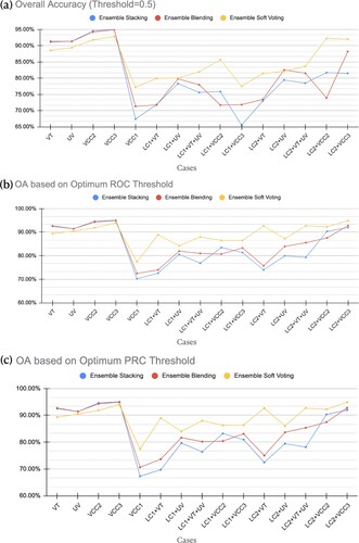
Table 8. Overall accuracy (threshold $=0.5$) of ensemble models for different cases.

Cases	Ensemble Stacking	Ensemble Blending	Ensemble Soft Voting
VT	91.14%	91.32%	88.58%
UV	91.34%	91.32%	89.39%
VCC2	94.57%	94.21%	91.76%
VCC3	95.00%	94.91%	92.86%
VCC1	67.40%	71.31%	77.18%
LC1 + VT	71.88%	71.77%	79.93%
LC1 + UV	78.33%	79.78%	80.02%
LC1 + VT + UV	75.59%	77.97%	81.94%
LC1 + VCC2	75.86%	71.69%	85.67%
LC1 + VCC3	65.53%	71.83%	77.50%
LC2 + VT	73.00%	73.46%	81.44%
LC2 + UV	79.43%	82.55%	82.10%
LC2 + VT + UV	78.46%	81.53%	83.64%
LC2 + VCC2	81.69%	73.91%	92.23%
LC2 + VCC3	81.48%	88.20%	92.00%

Table 9. Overall accuracy based on optimum ROC-based thresholds of ensemble models for different cases.

Cases	Ensemble Stacking		Ensemble Blending		Ensemble Soft Voting
	OA	Threshold	OA	Threshold	OA	Threshold
VT	92.73%	0.1890	92.52%	0.2374	89.37%	0.4280
UV	91.44%	0.4418	91.45%	0.4624	90.41%	0.3869
VCC2	94.65%	0.5482	94.29%	0.5396	91.88%	0.4822
VCC3	95.01%	0.4996	94.92%	0.4876	93.91%	0.6190
VCC1	70.21%	0.6496	72.47%	0.5889	77.39%	0.4860
LC1 + VT	72.59%	0.5117	73.96%	0.3790	88.94%	0.1935
LC1 + UV	80.56%	0.3285	81.94%	0.3527	84.20%	0.4307
LC1 + VT + UV	76.84%	0.3484	80.99%	0.3536	87.98%	0.3487
LC1 + VCC2	83.48%	0.8515	80.70%	0.8597	86.46%	0.6030
LC1 + VCC3	81.33%	0.9483	83.30%	0.9044	86.48%	0.7534
LC2 + VT	73.99%	0.5117	75.72%	0.3790	92.64%	0.1741
LC2 + UV	79.94%	0.3959	83.97%	0.4008	87.25%	0.4205
LC2 + VT + UV	79.29%	0.4394	85.53%	0.3064	92.71%	0.2061
LC2 + VCC2	90.34%	0.7842	87.56%	0.8324	92.25%	0.4898
LC2 + VCC3	91.97%	0.8249	92.78%	0.7787	94.88%	0.6049

Table 10. Overall accuracy based on optimum PRC-based thresholds of ensemble models for different cases.

Cases	Ensemble Stacking		Ensemble Blending		Ensemble Soft Voting
	OA	Threshold	OA	Threshold	OA	Threshold
VT	92.73%	0.1850	92.52%	0.2170	89.34%	0.3917
UV	91.38%	0.3000	91.44%	0.3396	90.42%	0.3680
VCC2	94.64%	0.5137	94.29%	0.5396	91.86%	0.4398
VCC3	95.01%	0.4996	94.92%	0.4876	93.91%	0.6190
VCC1	67.31%	0.4629	70.63%	0.4044	77.39%	0.4860
LC1 + VT	69.73%	0.3419	73.64%	0.3296	88.94%	0.1932
LC1 + UV	79.65%	0.2273	81.69%	0.2854	84.01%	0.4175
LC1 + VT + UV	76.40%	0.2863	80.18%	0.2429	87.98%	0.3487
LC1 + VCC2	83.22%	0.8012	80.39%	0.8162	86.30%	0.5537
LC1 + VCC3	80.94%	0.9204	83.10%	0.8775	86.36%	0.7293
LC2 + VT	72.46%	0.4245	75.00%	0.3296	92.64%	0.1739
LC2 + UV	79.44%	0.3478	83.64%	0.3525	86.05%	0.2647
LC2 + VT + UV	78.16%	0.3270	85.35%	0.2630	92.68%	0.1926
LC2 + VCC2	90.31%	0.7708	87.44%	0.8156	92.23%	0.4691
LC2 + VCC3	91.96%	0.8111	92.76%	0.7627	94.87%	0.5949

Disregarding the chosen threshold, stacking and blending methods produced similar performance and displayed the best accuracy (i.e. $\mathrm{OA}=0.91\sim 0.93$ for VT, $\mathrm{OA}=0.92$ for UV, and $\mathrm{OA}=0.94\sim 0.95$ for both VCC2 and VCC3) compared to SV (i.e. $\mathrm{OA}=0.88\sim 0.89$ for VT, $\mathrm{OA}=0.89\sim 0.9$ for UV, and $\mathrm{OA}=0.91\sim 0.94$ for both VCC2 and VCC3) when the data sampled in a region was used to train the model (i.e. VT, UV, VCC2, and VCC3). When the data sampled in an area was not used to train the model (i.e. VCC1, LC1, and LC2), the SV model outperformed other models. Additionally, blending also performed well in terms of accuracy (i.e. $\mathrm{OA}=0.71\sim 0.72$ for VCC1, and $\mathrm{OA}=0.72\sim 0.93$ for both LC1 and LC2) in this case and was marginally superior to stacking (i.e. $\mathrm{OA}=0.67\sim 0.7$ for VCC1, and $\mathrm{OA}=0.66\sim 0.92$ for both LC1 and LC2).

Both the staking and blending models offered comparable accuracy for Val Tartano and Upper Vatellina and outperformed the SV model. When utilizing the optimum threshold, the stacking model trained on the dataset only sampled in Valchiavenna (VCC3) demonstrated the best performance for Valchiavenna with a maximum overall accuracy of 0.95. With a maximum overall accuracy improvement of 0.12, the SV model trained in VCC3 ($\mathrm{OA}=0.78$ for LC1 + VCC3) outperformed the stacking model trained in VCC3 ($\mathrm{OA}=0.66$ for LC1 + VCC3) in Lombardy instances and provided the best performance when the optimum threshold is adopted ($\mathrm{OA}=0.95$ for LC2 + VCC3).

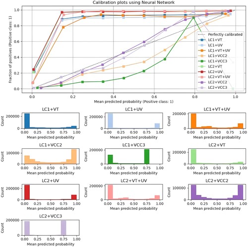
Overall, the Neural Network outperformed all other models at estimating a landslide probability occurrence when all outputs for Lombardy cases were compared, with the highest overall accuracy being 0.97. The calibration plots for the various Neural Network models tested in Lombardy are depicted in Figure 16. Notably, only the Neural Network model trained on VCC2 exhibits improvement upon the calibration, therefore, it was chosen as the final model to generate LSM for Lombardy.

Figure 16. Calibration plots for Neural Network models applied on Lombardy case.

3.3. Result of the introduction of precipitation as an environmental factor

Precipitation was added to the Neural Network as a new factor in VCC2 case. In this situation, three additional NN models were trained individually utilizing average precipitation, the 90th percentile of precipitation, and both average and 90th percentile precipitation. The performance of the constructed models was then assessed by applying them to the Lombardy cases (i.e. LC1 and LC2). Table 11 reports the accuracy estimation based on several threshold types with or without input from precipitation.

Table 11. Accuracy statistic of Neural Network with or without precipitation as input based on threshold 0.5 and optimum thresholds based on ROC and PRC.

Cases		VCC2	LC1 + VCC2	LC2 + VCC2
Neural Network without precipitation	Base OA	89.01%	85.83%	93.10%
	Optimal ROC OA	89.05%	87.11%	93.13%
	Optimal PRC OA	88.96%	87.03%	93.10%
Neural Network with average precipitation	Base OA	87.72%	87.96%	91.08%
	Optimal ROC OA	88.46%	90.16%	95.93%
	Optimal PRC OA	88.46%	90.16%	95.93%
Neural Network with 90th percentile precipitation	Base OA	87.92%	87.57%	91.04%
	Optimal ROC OA	88.54%	89.54%	95.29%
	Optimal PRC OA	88.37%	89.53%	95.29%
Neural Network with both average and 90th percentile precipitation	Base OA	87.96%	88.03%	91.80%
	Optimal ROC OA	88.74%	88.86%	95.77%
	Optimal PRC OA	88.72%	88.85%	95.77%

When the model was trained and applied to the same area (i.e. VCC2), there was no comparable accuracy difference with or without precipitation as an additional factor; however, the model trained with added precipitation yields an accuracy improvement of around 2–3% for the Lombardy case (i.e. LC1 and LC2), where the maximum accuracy improvement was found in the model trained only with the average precipitation included.

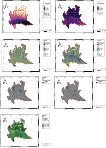
3.4. Landslide susceptibility mapping

Two different schemas were used to categorize the probability values of ML models into different susceptibility classes:

•	Four classes: low $[0,0.25]$, medium $(0.25,0.5]$, high $(0.5,0.75]$, very high $(0.75,1]$;
•	Five classes, modified upon Van-Den-Eeckhaut et al. (2012) and Guzzetti et al. (2006): very low $[0,0.2]$, low $(0.2,0.45]$, medium $(0.45,0.55]$, high $(0.55,0.9]$, very high $(0.9,1]$.

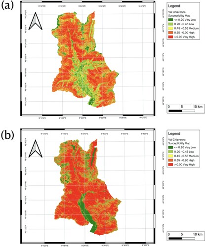
Figures 17 and 18 displays the landslide susceptibility maps for each basin based on the top-performing ML models (RF models with a hyperparameter (i.e. number of decision trees) set to 100) for each basin scenario. Figure 18(a) also displays the outcomes of the first-time application of a model that was trained on one region to another (i.e. VCC1). Although the model was not built using any data from this area, the accuracy for this situation is close to 0.75, demonstrating good generalization.

Figure 17. Landslide susceptibility maps for Val Tartano and Upper Valtellina: a LSM for Val Tartano derived from Random Forests model trained in VT; b LSM for Upper Valtellina derived from Random Forests model trained in UV.

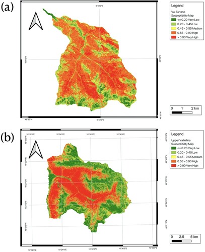
Figure 18. Landslide susceptibility maps for Valchiavenna: a LSM for Valchiavenna derived from Random Forests model trained in VCC1; b LSM for Valchiavenna derived from Random Forests model trained in VCC3.

The best-performing ML models trained on VCC2 (The NN models. The tuned hyperparameters, that is, the size, activation function, and the initial learning rate were set to 100, the logistic sigmoid function and 0.001, respectively) with added average precipitation data and without precipitation data were used to map the landslide susceptibility of Lombardy (Figures 19 and 20). Please note that the presence of clusters with mainly high or low susceptibility in the LSMs shown in the figures is a visualization matter arising from the scale and dimensions of the figures.

Figure 19. Landslide susceptibility maps of Lombardy using 4-classes schema: a LSM derived from Neural Network model trained in VCC2 without precipitation data; b LSM derived from Neural Network model trained in VCC2 with average precipitation data.

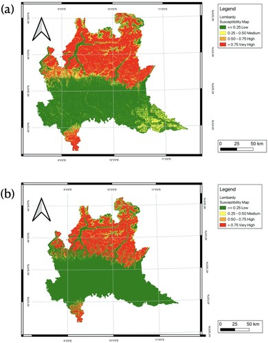
Figure 20. Landslide susceptibility maps of Lombardy using 5-classes schema: a LSM derived from Neural Network model trained in VCC2 without precipitation data; b LSM derived from Neural Network model trained in VCC2 with average precipitation data.

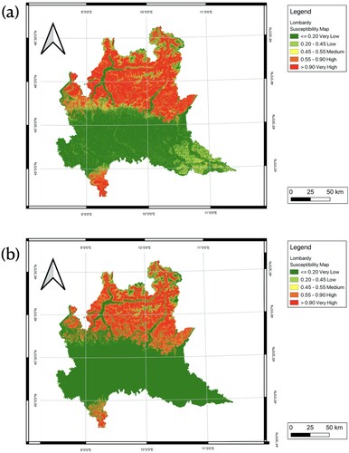
The resulting LSMs were consistent with the fact that all considered landslides documented in the landslide inventory occurred north of Lombardy. A high and very high susceptibility is also present in the south part of Lombardy (the southern part of the Po River), despite the fact that there are no records of landslides there. The central foothills of Lombardy are in regions of extremely low or low susceptibility when the precipitation data was not taken into account in the model. Using the same model, the exclusion of precipitation data resulted in certain land parcels in southeast Lombardy being categorized as having a medium susceptibility under the 4-classes schema instead of the 5-classes schema, which classified these land parcels as having low susceptibility. However, upon incorporating the average precipitation into the model, both the central foothills and the southeast region of Lombardy were classified as having very low susceptibility using the 5-classes schema, or alternatively, low susceptibility under the 4-classes schema, with no observed variations.

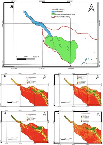
In order to evaluate the quality of the LSM, the largest landslide in Val Tartano, the Pruna landslide, was considered. The motivation for this is two-fold: on one hand, the Pruna is a Deep-seated Gravitational Slope Deformation (therefore not included in the used inventory), however, it hosts many overlaying shallow landslides. On the other hand, the inventory depicts a ‘debris flow’ (Figure 21(a)) which in reality is a debris deposit. Regardless of the model and schema employed, the region of this landslide is correctly classified as high and very high risk (Figure 21), while the debris deposit area depicts a lower probability of landslide occurrence (Figure 21(e)).

Figure 21. Pruna landslides: a The Pruna landslides and the debris flow; b The LSM derived from the VCC2+NN models without precipitation using a 4-classes schema; c The LSM derived from same model as b but using a 5-classes schema; d The LSM derived from the VCC2+NN models with average precipitation using a 4-classes schema; e The LSM derived from the same model as d but using a 5-classes schema.

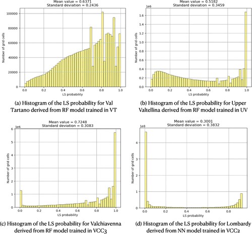
Additionally we have computed the mean value and standard deviation of the predicted probabilities for each of the case studies for their best-performing training input and ML model combination Figure 22, as they are used to analyze the uncertainties and variations of landslide susceptibility prediction modeling (Huang et al. 2020, 2023). From the three basins' histograms, it is evident the models' confidence as they are very particular cases with predominantly inclined alpine areas with a high density of landslide event records. On the other hand, the low mean value for the Lombardy case study depicts the zero effect of the Po basin lowlands and the particular lack of slope failures. In all four cases, the low standard deviation values indicate consistent models' confidence across all predictions and low levels of uncertainty.

Figure 22. Landslide susceptibility distribution features of the best model for each study area.

The spatial statistics of landslide susceptibility and the corresponding percentage of documented landslides in each susceptibility class derived from these models are presented in Tables 12 and 13. The spatial statistics of susceptibility maps indicated that when precipitation data was not included, 21.21% (i.e. 5070.66 km${}^2$) and 15.46% (i.e. 3696.34 km${}^2$) of the total area fell within very high and high landslide susceptibility categories respectively when adopting the 5-classes schema. Under this schema, very low, low, and medium susceptibility zones make up 48.93%, 11.93%, and 2.48%, respectively. When the 4-class schema was used, Lombardy had a susceptibility to landslides of 52.65%, which was 13.19% lower than the 4-class schema when taking into account the extremely low and low categories jointly. Only a little section of the Lombardy region was categorized as medium, with 9.47% of the overall area utilizing a 4-classes schema, a larger value with respect to the 5-classes schema. Regions with high and very high susceptibility accounted for about 37.88% of the territory of Lombardy, which is also somewhat larger than the corresponding value using the 5-classes schema.

Table 12. Distribution of susceptibility classes and landslides for Lombardy using 4-classes.

Susceptibility Class	LSM derived using VCC2+NN without precipitation			LSM derived using VCC2+NN with average precipitation
	Area	Area Percentage	Landslide Percentage	Area	Area Percentage	Landslide Percentage
Low	12589.93	52.65%	6.03%	15250.58	63.78%	11.43%
Medium	2263.52	9.47%	8.04%	1055.55	4.41%	10.25%
High	1593.00	6.66%	11.71%	1290.97	5.40%	13.21%
Very High	7464.30	31.22%	74.22%	6313.64	26.41%	65.10%

The unit of area is km${}^2$

Table 13. Distribution of susceptibility classes and landslides for Lombardy using 5-classes.

Susceptibility Class	LSM derived using VCC2+NN without precipitation			LSM derived using VCC2+NN with average precipitation
	Area	Area Percentage	Landslide Percentage	Area	Area Percentage	Landslide Percentage
Very Low	11698.81	48.93%	3.79%	14867.34	62.18%	8.31%
Low	2852.74	11.93%	8.74%	1253.03	5.24%	11.42%
Medium	592.22	2.48%	3.16%	378.88	1.58%	3.92%
High	3696.34	15.46%	35.04%	4320.16	18.07%	45.09%
Very High	5070.66	21.21%	49.27%	3091.34	12.93%	31.26%

The unit of area is km${}^2$

When average precipitation data was taken into account, a larger region was categorized as a low (i.e. 63.78% in 4-classes schema) and very low (i.e. 62.18% in 5-classes schema) susceptible area. The high and very high susceptible areas, on the other hand, were reduced (i.e. 5.4% of the high susceptible area and 26.41% of the very high susceptible area in the 4-classes schema, and 12.93% of the very high susceptible area in the 5-classes schema).

Almost 94% of the historical landslide locations in the 4-classes schema and 87% in the 5-classes schema fall into the range of medium to extremely high landslide susceptibility derived from the model built without using precipitation data. The percentage dropped to about 89% in the 4-class schema and 80% in the 5-class schema when average precipitation data were taken into account.

4. Discussion

4.1. Discussion about the results

The performance assessment highlighted five distinct and best-performing basic ML models for both basin-level LSM and regional LSM, utilizing various sets of testing data points. The majority of these models exhibited favourable estimates of the class probabilities, with the exception of Adaboost. Consequently, calibration emerges as an indispensable procedure when incorporating Adaboost into the analysis.

The performance of Valchiavenna case 3 (VCC3) in overall exceeds that of Valchiavenna case 2 (VCC2), despite the larger sample size of training points in VCC2. To explore this trend further, we analyzed the distribution of input factors in the training dataset for both VCC2 (Upper Valtellina + Val Tartano + Valchiavenna) and VCC3 (Valchiavenna), as well as in the testing dataset for both cases. It is noteworthy that the testing dataset remains constant for both cases. We also compared these distributions to the training dataset in VCC2, excluding the Valchiavenna part (Upper Valtellina + Val Tartano). The heterogeneity in the distribution of input factors observed between the training and testing datasets of VCC2, as opposed to the homogeneity observed in VCC3, indicates that the inclusion of additional samples from Upper Valtellina and Val Tartano introduces some noise into the training model. This fact indicates that an increase in data volume does not necessarily result in enhanced accuracy.

The findings depicted in Table 5 and Figure 14 reveal that Bagging, Random Forest (RF), and Gradient Tree Boosting models exhibit very good performance ($\mathrm{OA}>0.9$) when the model is applied in the corresponding area. However, in terms of generalization, the performance of Bagging and Gradient Tree Boosting models experiences a decline, while RF continues to maintain a strong performance ($\mathrm{OA}>0.8$, except in the VCC1 case). Despite Adaboost displaying slightly inferior performance in the former scenario, it demonstrates a superior ability to generalize compared to Bagging and Gradient Tree Boosting models.

In this study, various ensemble ML models were constructed by combining individual ML models that exhibited superior generalization performance. Notably, SV methods underperformed Stacking and Blending methods, with the latter achieving an OA exceeding 0.9 when tested within the same area as the training points. However, SV methods showcased their strengths in terms of generalization ability ($\mathrm{OA}>0.8$, except in the VCC1 case), outperforming Stacking and Blending methods.

Interestingly, in situations where both the training and test data points reside within the same region, the NN demonstrates a lower level of performance compared to the other models, even the ensemble modes. However, in the inverse scenario, the neural network surpasses the performance of the other models. More specifically, the OA based on the optimal threshold of the neural network rises from approximately 0.85 to around 0.95 when evaluating its ability to generalize. Nonetheless, the underlying causes for the neural network's underfitting behaviour remain unknown, necessitating further investigation. Besides, the NN model trained in VCC2 exhibits the best estimates of the class probabilities, therefore chosen as the final model for LSM.

Feature selection plays a crucial role in machine learning by eliminating redundant and less valuable variables to mitigate the risk of overfitting and enhance generalization. In our pursuit to assess the impact of precipitation on LSM, we incorporate various forms of precipitation data as supplementary features and retrain the NN model using the training datasets from the three basins. Through performance evaluation, we observed that the inclusion of precipitation as a feature yields a modest enhancement in the model's generalization capabilities. Specifically, in the Lombardy case, we witness an accuracy improvement of approximately 2-3%. Among the models trained using different types of precipitation data, the average precipitation data stands out as the most effective.

In general, the recorded landslide events ought to predominantly manifest in regions of very high or high susceptibility, while non-landslide samples should primarily populate safe areas characterized by low or very low susceptibility. Furthermore, the generated landslide susceptibility maps clearly delineate areas exhibiting extremely high and highly susceptible environmental settings toward landslide occurrences. The map derived from the NN model, excluding precipitation, revealed a considerable area (approximately 38% coverage in the 4-class schema and around 37% coverage in the 5-class schema) within Lombardy that exhibited very high or high susceptibility to landslides. This coverage surpassed the predictions (approximately 32% coverage in the 4-class schema and around 31% coverage in the 5-class schema) from the model incorporating precipitation, primarily concentrated in Lombardy's northern region. Around 49% and 62% of the total area in the NN models with and without precipitation data, respectively, exhibited very low susceptibility levels, with a prevalence of territory in Lombardy's central part. Furthermore, upon comparing these results, it becomes evident that while the NN model incorporating precipitation data exhibited slightly enhanced predictions compared to the NN model without precipitation, the NN model without precipitation demonstrated greater consistency and exhibited a closer agreement with the landslide database used for constructing the model. This was particularly evident as the model without precipitation data managed to encompass a larger number of historical landslide locations within the range of medium to extremely high landslide susceptibility. This valuable information can prove immensely beneficial for concerned authorities, decision-makers, and local residents, enabling them to make informed decisions regarding activities conducted within the landslide-prone areas. By being aware of the landslide risk and its potential consequences, appropriate measures can be implemented to safeguard lives and property. Concurrently, areas predicted to have lower susceptibility levels can maintain their protection by adhering to environmental guidelines, ensuring safety and security.

In general, the incorporation of more precise and robust Machine Learning techniques can undoubtedly enhance the effectiveness of landslide susceptibility studies. For this specific study, improvements could be made by incorporating a multitemporal landslide inventory and factoring in time as a variable in the analysis. Furthermore, refining the definition of the NoLsZ could yield significant benefits in the analysis.

Additionally, in this study, the models were specifically tailored for the Lombardy region, focusing solely on shallow landslides. Expanding the scope to encompass other regions or different types of landslides could lead to more insightful and comprehensive outcomes. The commitment to openness not only strengthens the reliability of our findings but also contributes to the broader goal of creating a more inclusive and collaborative scientific environment for addressing geohazard challenges. This is further supported by implementing the proposed framework using FOSS and open data, which can potentially lead to an increase in other case studies implementing and tuning this approach according to various research tasks. However, it is essential to consider that enlarging the study region may increase the computational complexity of prediction, making it less conducive to near real-time (NRT) LSM. To address this, techniques like distributed computing could be explored and implemented to accelerate the process and enable more efficient NRT LSM.

4.2. General discussion

An innovative aspect of this study is the utilization of a reverse-pyramid approach in machine learning model generalization. This method involves initiating the process by constructing a generic model on a basin scale. Subsequently, it integrates information from various basins to directly fine-tune a generalized model capable of predicting landslide susceptibility levels on a regional scale. The motivation of such implementation is two-folded, on one hand, some scholars have pointed out that the majority of the published works in the landslide susceptibility field are mainly focused on developing models and frameworks for site-specific case studies without tunning and testing them for areas that can share environmental characteristics (Sun et al. 2020; Z. Wang, Goetz, and Brenning 2022). On the other hand, by developing frameworks for generalized landslide susceptibility mapping can aid directly local authorities and decision-makers in cases when reliable input data (e.g. landslide inventories, environmental data) is lacking in areas that potentially could be affected by the hazard (Bandara et al. 2020). However, it should be emphasized that neither the presented here approach nor other produced by the community are expected to fit in the concept of one unified master algorithm, as simply the landslide hazard problem differs by its nature (e.g. predisposing, triggering, environmental factors). Nevertheless, developing generalized models for specific landslide typologies or terrain characteristics is certainly a recommendation for future studies.

Additionally, the introduction of a No Landslide Zone represents a valuable and innovative feature. This zone is identified through geological criteria, aiming to pinpoint areas with an extremely low likelihood of landslides. This supplementary information enriches the model's dataset by including details about the absence of landslides. Such information is frequently overlooked in the literature, yet its inclusion has proven to fortify the model and generate more reliable outcomes. The direct evaluation of the proposed hypothesis for determining areas with very low shallow landslide probability (NoLsZ) and its very low estimated errors proved that it can be successfully applied for delineating and further sampling the null cases for the machine learning models. Hence the expectancy of more reliable susceptibility models. The overlapping NoLsZ areas with the landslide inventory highlight some disagreement between the stable areas and failed slope but most of them can be directly related to the accuracy of the landslide delineation and/or displaced deposits. It is important to stress that the hypothesis is specifically tailored for the case study of the Lombardy region and shallow landslides, therefore, we do not encourage its direct application in other regions or for modeling different types of landslides without its revision from an expert. The involvement of geologists with local knowledge of the area is the aspect that we consider robust, similar to the fact that the positive case (landslide inventory) is also compiled by experts in the field. Another positive aspect is the need for fewer input data in comparison to already proposed statically methods (e.g. (Sun et al. 2023)), which on the other hand are bringing a solution that performs well with scalability and (Jia et al. 2021; Marchesini et al. 2014), which can be considered as limiting factor in the here proposed approach.

With the use of several evaluation indices, such as overall accuracy, precision, recall, ROC, and PRC, the performance of each ML model was assessed in a variety of scenarios, including VT, UV, VCC1, VCC2, VCC3, LC1, and LC2 (Section 2.3.1), which fits in the community urge for the implementation of more diverse and suitable evaluation frameworks (Fleuchaus et al. 2021; Yong et al. 2022; Yordanov and Brovelli 2020, 2021). The models with the best performance in the cases where sampled data from the corresponding area were not used for model training (RF, Calibrated AdaBoost, and NN) were chosen as the base classifiers for ensemble models. When compared to their base classifiers, the ensemble models' statistical performance did not significantly improve, however, could be considered consistent among them which aligns with other works (Di Napoli et al. 2020; Rokach 2010). Although the Neural Network model had lower performance when trained using data from the basin regions, it outperformed all other generated models in terms of generalization ability.

When precipitation data was not taken into account, the susceptibility map created using Neural Network constructed in VCC2 for the Lombardy region indicated that almost 37% of the whole study area fell between the ‘very high’ and ‘high’ landslide susceptibility categories. When the average precipitation data were added, this percentage dropped to 31%. However, the implementation of precipitation in the susceptibility mapping is currently not very well defined in the literature, as some authors are implementing it as cumulative rainfall for a certain period (Xing et al. 2021). Others are tailoring it according to the landslide occurrence date from the inventory (B. Li et al. 2022), where the latter should be depicting more accurately the triggering mechanism, however such implementation can be challenging as few landslide inventories are simultaneously rich of entries and precise in terms of location and time.

5. Conclusion

Identification of landslide-prone areas can be valuable for land use planners or disaster management agencies in allocating resources to forecast and mitigate landslide impacts. The presented work covers a wide range of susceptibility modeling scenarios using five base classification methods and three ensemble techniques on three basins and extends to the whole Lombardy region. 11 factors (e.g. elevation, eastness, northness, NDVI, etc.) were initially used to train and determine the final model, followed by the incorporation of precipitation data into the final model. This work attempted to tackle several issues that are sometimes overlooked or inherently omitted by other works in the landslide hazard domain, namely, the sampling approach for the input of zero-case datasets (locations where the possibility of landslide occurrence is very low) and testing the generalization performance of the developed ML models. In this work, we have proposed a No Landslide Zone as a knowledge-based solution to the former issue which provided more than satisfactory results, however, its application may not be straightforward when scaling or changing the case study, environmental characteristics or landslide typology. In reference to the second issue, we have implemented a combination of training sets and models to generate an ML model that has the best (among the ones developed by us) generalized predictive performance. By such we have demonstrated that it is feasible to train a landslide susceptibility model using limited basin information and obtain highly accurate predictions on a regional scale. The landslide susceptibility maps generated in this study hold the potential to be utilized by policymakers in devising an effective mitigation strategy to minimize landslide risks, fostering the sustainable development of the area.

Author Contributions

Conceptualization, M.A.B., V.Y., Q.X. and L.A.; methodology, M.A.B., V.Y. and Q.X.; software, V.Y. and Q.X.; validation, Q.X.; formal analysis, M.A.B., V.Y. and Q.X.; investigation, Q.X.; resources, V.Y. and Q.X.; data curation, V.Y. and Q.X.; writing – original draft preparation, Q.X. and L.A.; writing – review and editing, M.A.B. and V.Y.; visualization, Q.X.; supervision, M.A.B. and V.Y.; project administration, M.A.B.; funding acquisition, M.A.B. All authors have read and agreed to the published version of the manuscript.

Code availability

The code is available at GEOlab Github - Landslide Susceptibility Mapping

Disclosure statement

No potential conflict of interest was reported by the author(s).

Data availability statement

The data that support the findings of this study are openly available in Zenodo. The relevant input datasets are available at https://doi.org/10.5281/zenodo.8185734.

 Google Scholar

, the outputs from ensemble machine learning models are available at https://doi.org/10.5281/zenodo.8185870,

 Google Scholar

. The estimated No Landslide Zone for Lombardy Regions is available at https://doi.org/10.5281/zenodo.8185887

 Google Scholar

.

Additional information

Funding

This research is partially funded by the Italian Ministry of Foreign Affairs and International Cooperation within the project ‘Geoinformatics and Earth Observation for Landslide Monitoring’ CUP D19C21000480001.

Appendices

Appendix 1.

Other accuracy statistics of base classifiers for different cases

Table A1. Precision of base classifiers for different cases.

Cases	Bagging	Random Forest	AdaBoost	AdaBoost Calibrated	Gradient Tree Boosting	Neural Network
VT	0.9361	0.9483	0.8507	0.8545	0.9197	0.8482
UV	0.9466	0.9482	0.8944	0.9010	0.9164	0.9033
VCC2	0.9378	0.9361	0.8707	0.8718	0.9273	0.8653
VCC3	0.9441	0.9460	0.9109	0.9111	0.9495	0.7972
VCC1	0.6870	0.7501	0.7856	0.7863	0.6821	0.8419
LC1 + VT	0.8918	0.9197	0.9386	0.9394	0.9145	0.9451
LC1 + UV	0.7618	0.8958	0.7087	0.7297	0.5777	0.9386
LC1 + VT + UV	0.8761	0.9147	0.9324	0.9319	0.8974	0.9412
LC1 + VCC2	0.7021	0.7505	0.7504	0.7505	0.6681	0.8206
LC1 + VCC3	0.6142	0.6131	0.5643	0.5617	0.5731	0.8611
LC2 + VT	0.9657	0.9754	0.9865	0.9867	0.9753	0.9887
LC2 + UV	0.7400	0.9588	0.7717	0.7895	0.6368	0.9873
LC2 + VT + UV	0.9574	0.9777	0.9855	0.9853	0.9299	0.9879
LC2 + VCC2	0.7676	0.8668	0.8401	0.8488	0.7498	0.9424
LC2 + VCC3	0.8468	0.7416	0.5326	0.5305	0.6592	0.9664

Table A2. Recall of base classifiers for different cases.

Cases	Bagging	Random Forest	AdaBoost	AdaBoost Calibrated	Gradient Tree Boosting	Neural Network
VT	0.8715	0.8810	0.8690	0.8665	0.8765	0.7010
UV	0.8640	0.8662	0.8708	0.8683	0.8716	0.8333
VCC2	0.9502	0.9518	0.9303	0.9294	0.9398	0.9241
VCC3	0.9516	0.9559	0.9361	0.9363	0.9456	0.9746
VCC1	0.7082	0.7544	0.7927	0.7912	0.6896	0.7302
LC1 + VT	0.6847	0.5825	0.6139	0.6210	0.3260	0.4669
LC1 + UV	0.4923	0.5962	0.8792	0.8633	0.7842	0.5545
LC1 + VT + UV	0.5045	0.6029	0.7533	0.7560	0.4534	0.5480
LC1 + VCC2	0.9419	0.9379	0.9248	0.9248	0.9279	0.9172
LC1 + VCC3	0.9736	0.9743	0.9641	0.9671	0.9162	0.9736
LC2 + VT	0.6849	0.5842	0.6153	0.6219	0.3260	0.4702
LC2 + UV	0.4933	0.5970	0.8800	0.8646	0.7837	0.5548
LC2 + VT + UV	0.5059	0.6045	0.7524	0.7553	0.4543	0.5485
LC2 + VCC2	0.9419	0.9375	0.9258	0.9259	0.9278	0.9182
LC2 + VCC3	0.9746	0.9750	0.9651	0.9681	0.9164	0.9740

Table A3. $F_1$ score of base classifiers for different cases.

Cases	Bagging	Random Forest	AdaBoost	AdaBoost Calibrated	Gradient Tree Boosting	Neural Network
VT	0.9026	0.9134	0.8598	0.8605	0.8976	0.7676
UV	0.9034	0.9054	0.8825	0.8843	0.8935	0.8669
VCC2	0.9439	0.9439	0.8995	0.8997	0.9335	0.8937
VCC3	0.9478	0.9509	0.9233	0.9235	0.9475	0.8770
VCC1	0.6974	0.7523	0.7892	0.7887	0.6858	0.7821
LC1 + VT	0.7746	0.7133	0.7423	0.7477	0.4806	0.6250
LC1 + UV	0.5981	0.7159	0.7848	0.7909	0.6653	0.6972
LC1 + VT + UV	0.6403	0.7268	0.8333	0.8348	0.6024	0.6927
LC1 + VCC2	0.8045	0.8338	0.8286	0.8286	0.7768	0.8662
LC1 + VCC3	0.7532	0.7526	0.7119	0.7106	0.7051	0.9139
LC2 + VT	0.8014	0.7307	0.7579	0.7629	0.4887	0.6373
LC2 + UV	0.5920	0.7358	0.8223	0.8253	0.7026	0.7104
LC2 + VT + UV	0.6620	0.7470	0.8533	0.8551	0.6104	0.7054
LC2 + VCC2	0.8459	0.9007	0.8809	0.8857	0.8294	0.9301
LC2 + VCC3	0.9062	0.8424	0.6864	0.6854	0.7668	0.9702

Appendix 2.

Other accuracy statistics of ensemble classifiers for different cases

Table A4. Precision of ensemble models for different cases.

Cases	Ensemble Stacking	Ensemble Blending	Ensemble Soft Voting
VT	0.9456	0.9472	0.9164
UV	0.9371	0.9394	0.9386
VCC2	0.9354	0.9355	0.9055
VCC3	0.9477	0.9461	0.8973
VCC1	0.6464	0.6805	0.7761
LC1 + VT	0.7670	0.8520	0.9457
LC1 + UV	0.8539	0.8522	0.9157
LC1 + VT + UV	0.8441	0.8613	0.9421
LC1 + VCC2	0.6876	0.6495	0.8176
LC1 + VCC3	0.5949	0.6447	0.6938
LC2 + VT	0.7873	0.8997	0.9882
LC2 + UV	0.8776	0.9113	0.9701
LC2 + VT + UV	0.9133	0.9462	0.9875
LC2 + VCC2	0.7509	0.6699	0.9249
LC2 + VCC3	0.7388	0.8230	0.8717

Table A5. Recall of ensemble models for different cases.

Cases	Ensemble Stacking	Ensemble Blending	Ensemble Soft Voting
VT	0.8775	0.8795	0.8550
UV	0.8875	0.8845	0.8443
VCC2	0.9576	0.9498	0.9324
VCC3	0.9525	0.9525	0.9679
VCC1	0.7682	0.8032	0.7640
LC1 + VT	0.6284	0.5269	0.6351
LC1 + UV	0.6836	0.7205	0.6614
LC1 + VT + UV	0.6278	0.6666	0.6806
LC1 + VCC2	0.9479	0.9420	0.9181
LC1 + VCC3	0.9733	0.9726	0.9843
LC2 + VT	0.6302	0.5282	0.6363
LC2 + UV	0.6840	0.7212	0.6624
LC2 + VT + UV	0.6290	0.6686	0.6815
LC2 + VCC2	0.9482	0.9427	0.9193
LC2 + VCC3	0.9741	0.9734	0.9850

Table A6. $F_1$ score of ensemble models for different cases.

Cases	Ensemble Stacking	Ensemble Blending	Ensemble Soft Voting
VT	0.9103	0.9121	0.8846
UV	0.9116	0.9111	0.8890
VCC2	0.9464	0.9426	0.9188
VCC3	0.9501	0.9493	0.9313
VCC1	0.7021	0.7368	0.7700
LC1 + VT	0.6908	0.6511	0.7599
LC1 + UV	0.7593	0.7808	0.7680
LC1 + VT + UV	0.7201	0.7516	0.7903
LC1 + VCC2	0.7970	0.7689	0.8650
LC1 + VCC3	0.7385	0.7754	0.8139
LC2 + VT	0.7000	0.6656	0.7742
LC2 + UV	0.7688	0.8052	0.7872
LC2 + VT + UV	0.7449	0.7835	0.8064
LC2 + VCC2	0.8381	0.7832	0.9221
LC2 + VCC3	0.8403	0.8919	0.9249

Appendix 3.

Maps of landslide influencing factors

Figure A1. Lombardy landslide influencing factors.

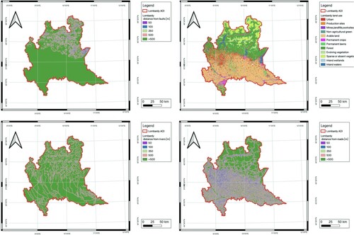
Figure A2. Lombardy landslide influencing factors (continue).

References

- Achu, A. L., C. D. Aju, M. Di Napoli, P. Prakash, G. Gopinath, E. Shaji, and V. Chandra. 2023. “Machine-Learning Based Landslide Susceptibility Modelling with Emphasis on Uncertainty Analysis.” Geoscience Frontiers 14 (6): 101657. https://doi.org/10.1016/j.gsf.2023.101657.
- Ado, M., K. Amitab, A. K. Maji, E. Jasińska, R. Gono, Z. Leonowicz, and M. Jasiński. 2022. “Landslide Susceptibility Mapping Using Machine Learning: A Literature Survey.” Remote Sensing 14 (13): 3029. https://doi.org/10.3390/rs14133029.
- Antonielli, B., P. Mazzanti, A. Rocca, F. Bozzano, and L. Dei Cas. 2019. “A-DInSAR Performance for Updating Landslide Inventory in Mountain Areas: An Example From Lombardy Region (Italy).” Geosciences 9 (9): 364. https://doi.org/10.3390/geosciences9090364.
- Azarafza, M., M. Azarafza, H. Akgün, P. M. Atkinson, and R. Derakhshani. 2021. “Deep Learning-Based Landslide Susceptibility Mapping.” Scientific Reports 11 (1): 24112. https://doi.org/10.1038/s41598-021-03585-1.
- Bajni, G., C. A. S Camera, A. Brenning, and T. Apuani. 2021. “Rock Mass Geomechanical Properties to Improve Rockfall Susceptibility Assessment: A Case Study in Valchiavenna (SO).” IOP Conference Series: Earth and Environmental Science 833 (1): 012180. https://doi.org/10.1088/1755-1315/833/1/012180.
- Bandara, A., Y. Hettiarachchi, K. Hettiarachchi, S. Munasinghe, I. Wijesinghe, and U. Thayasivam. 2020. “A Generalized Ensemble Machine Learning Approach for Landslide Susceptibility Modeling.” In Advances in Intelligent Systems and Computing, 71–93. Singapore, Springer. https://doi.org/10.1007/978-981-13-9364-8_6.
- Baradaran, R., and H. Amirkhani. 2021. “Ensemble Learning-Based Approach for Improving Generalization Capability of Machine Reading Comprehension Systems.” Neurocomputing 466:229–242. https://doi.org/10.1016/j.neucom.2021.08.095.
- Bradley, A. P. 1997. “The Use of the Area Under the ROC Curve in the Evaluation of Machine Learning Algorithms.” Pattern Recognition 30 (7): 1145–1159. https://doi.org/10.1016/S0031-3203(96)00142-2.
- Breiman, L. 1996. “Bagging Predictors.” Machine Learning 24 (2): 123–140. https://doi.org/10.1007/BF00058655.
- Brovelli, M. A., M. Minghini, R. Moreno-Sanchez, and R. Oliveira. 2017. “Free and Open Source Software for Geospatial Applications (FOSS4G) to Support Future Earth.” International Journal of Digital Earth10 (4): 386–404. https://doi.org/10.1080/17538947.2016.1196505.
- Budimir, M. E. A, P. M. Atkinson, and H. G. Lewis. 2015. “A Systematic Review of Landslide Probability Mapping Using Logistic Regression.” Landslides 12 (3): 419–436. https://doi.org/10.1007/s10346-014-0550-5.
- Coetzee, S., I. Ivánová, H. Mitasova, and M. Brovelli. 2020. “Open Geospatial Software and Data: A Review of the Current State and a Perspective into the Future.” ISPRS International Journal of Geo-Information 9 (2): 90. https://doi.org/10.3390/ijgi9020090.
- Colombera, L., and R. Bersezio. 2011. “Impact of the Magnitude and Frequency of Debris-Flow Events on the Evolution of An Alpine Alluvial Fan During the Last Two Centuries: Responses to Natural and Anthropogenic Controls.” Earth Surface Processes and Landforms 36 (12): 1632–1646. https://doi.org/10.1002/esp.2178.
- Cruden, D. 1991. “A Simple Definition of a Landslide.” Bulletin of the International Association of Engineering Geology -- Bulletin de l'Association Internationale de Géologie de l'Ingénieur 43 (1): 27–29. https://doi.org/10.1007/BF02590167.
- Cruden, D. M., and D. J. Varnes. 1996. Landslides: Investigation and Mitigation. Chapter 3-Landslide Types and Processes. Transportation research board special report (247).
- Di Napoli, M., F. Carotenuto, A. Cevasco, P. Confuorto, D. Di Martire, M. Firpo, G. Pepe, E. Raso, and D. Calcaterra. 2020. “Machine Learning Ensemble Modelling As a Tool to Improve Landslide Susceptibility Mapping Reliability.” Landslides 17 (8): 1897–1914. https://doi.org/10.1007/s10346-020-01392-9.
- Fang, Z., Y. Wang, L. Peng, and H. Hong. 2021. “A Comparative Study of Heterogeneous Ensemble-Learning Techniques for Landslide Susceptibility Mapping.” International Journal of Geographical Information Science 35 (2): 321–347. https://doi.org/10.1080/13658816.2020.1808897.
- Fleuchaus, P., P. Blum, M. Wilde, B. Terhorst, and C. Butscher. 2021. “Retrospective Evaluation of Landslide Susceptibility Maps and Review of Validation Practice.” Environmental Earth Sciences 80 (15): 485. https://doi.org/10.1007/s12665-021-09770-9.
- Freund, Y., and R. E. Schapire. 1997. “A Decision-Theoretic Generalization of On-Line Learning and An Application to Boosting.” Journal of Computer and System Sciences 55 (1): 119–139. https://doi.org/10.1006/jcss.1997.1504.
- Friedman, J. H. 2001. “Greedy Function Approximation: A Gradient Boosting Machine.” The Annals of Statistics 29 (5): 1189–1232. https://doi.org/10.1214/aos/1013203451.
- Friedman, J., T. Hastie, and R. Tibshirani. 2000. “Additive Logistic Regression: A Statistical View of Boosting (With Discussion and a Rejoinder by the Authors).” The Annals of Statistics 28 (2): 337–407. https://doi.org/10.1214/aos/1016218223.
- Ganaie, M. A., M. Hu, A. K. Malik, M. Tanveer, and P. N. Suganthan. 2022. “Ensemble Deep Learning: A Review.” Engineering Applications of Artificial Intelligence 115:105151. https://doi.org/10.1016/j.engappai.2022.105151.
- Guzzetti, F., A. Carrara, M. Cardinali, and P. Reichenbach. 1999. “Landslide Hazard Evaluation: A Review of Current Techniques and Their Application in a Multi-Scale Study, Central Italy.” Geomorphology 31 (1): 181–216. https://doi.org/10.1016/S0169-555X(99)00078-1.
- Guzzetti, F., P. Reichenbach, F. Ardizzone, M. Cardinali, and M. Galli. 2006. “Estimating the Quality of Landslide Susceptibility Models.” Geomorphology 81 (1–2): 166–184. https://doi.org/10.1016/j.geomorph.2006.04.007.
- Habumugisha, J. M., N. Chen, M. Rahman, M. M. Islam, H. Ahmad, A. Elbeltagi, G. Sharma, S. N. Liza, and A. Dewan. 2022. “Landslide Susceptibility Mapping with Deep Learning Algorithms.” Sustainability14 (3): 1734. https://doi.org/10.3390/su14031734.
- Huang, F., Z. Cao, J. Guo, S.-H. Jiang, S. Li, and Z. Guo. 2020. “Comparisons of Heuristic, General Statistical and Machine Learning Models for Landslide Susceptibility Prediction and Mapping.” Catena191:104580. https://doi.org/10.1016/j.catena.2020.104580.
- Huang, F., H. Xiong, C. Yao, F. Catani, C. Zhou, and J. Huang. 2023. “Uncertainties of Landslide Susceptibility Prediction Considering Different Landslide Types.” Journal of Rock Mechanics and Geotechnical Engineering 15 (11): 2954–2972. https://doi.org/10.1016/j.jrmge.2023.03.001.
- ISPRA. 2014. “IdroGEO -- Open Data.” https://idrogeo.isprambiente.it/app/page/open-data.
- ISTAT. 2020. “Territory and Population. -- Regional.” https://www.asr-lombardia.it/asrlomb/en/opendata/Territory\_and\_population\_\_\_Regional.
- Jia, G., M. Alvioli, S. L. Gariano, I. Marchesini, F. Guzzetti, and Q. Tang. 2021. “A Global Landslide Non-Susceptibility Map.” Geomorphology 389:107804. https://doi.org/10.1016/j.geomorph.2021.107804.
- Kadavi, P. R., C. W. Lee, and S. Lee. 2018. “Application of Ensemble-Based Machine Learning Models to Landslide Susceptibility Mapping.” Remote Sensing 10 (8): 1252. https://doi.org/10.3390/rs10081252.
- Kavzoglu, T., A. Teke, and E. O. Yilmaz. 2021. “Shared Blocks-Based Ensemble Deep Learning for Shallow Landslide Susceptibility Mapping.” Remote Sensing 13 (23): 4776. https://doi.org/10.3390/rs13234776.
- Kumar, C., G. Walton, P. Santi, and C. Luza. 2023. “An Ensemble Approach of Feature Selection and Machine Learning Models for Regional Landslide Susceptibility Mapping in the Arid Mountainous Terrain of Southern Peru.” Remote Sensing 15 (5): 1376. https://doi.org/10.3390/rs15051376.
- Li, W., Z. Fang, and Y. Wang. 2022. “Stacking Ensemble of Deep Learning Methods for Landslide Susceptibility Mapping in the Three Gorges Reservoirarea, China.” Stochastic Environmental Research and Risk Assessment 36 (8): 2207–2228. https://doi.org/10.1007/s00477-021-02032-x.
- Li, B., K. Liu, M. Wang, Q. He, Z. Jiang, W. Zhu, and N. Qiao. 2022. “Global Dynamic Rainfall-Induced Landslide Susceptibility Mapping Using Machine Learning.” Remote Sensing 14 (22): 5795. https://doi.org/10.3390/rs14225795.
- Lombardia, R. 2020. “Territory and Population.” https://www.en.regione.lombardia.it/wps/portal/site/en-regione-lombardia/discover-lombardy/territory-and-population.
- Longoni, L., M. Papini, D. Brambilla, L. Barazzetti, F. Roncoroni, M. Scaioni, and V. I. Ivanov. 2016. “Monitoring Riverbank Erosion in Mountain Catchments Using Terrestrial Laser Scanning.” Remote Sensing 8 (3): 241. https://doi.org/10.3390/rs8030241.
- Marchesini, I., F. Ardizzone, M. Alvioli, M. Rossi, and F. Guzzetti. 2014. “Non-Susceptible Landslide Areas in Italy and in the Mediterranean Region.” Natural Hazards and Earth System Sciences 14 (8): 2215–2231. https://doi.org/10.5194/nhess-14-2215-2014.
- Mobasheri, A., H. Mitasova, M. Neteler, A. Singleton, H. Ledoux, and M. A. Brovelli. 2020. “Highlighting Recent Trends in Open Source Geospatial Science and Software.” Transactions in GIS 24 (5): 1141–1146. https://doi.org/10.1111/tgis.12703.
- Moreno-Sanchez, R., and M. A. Brovelli. 2023. Free and Open Source Software for Geospatial Applications (FOSS4G). 1st ed., 246–255. London, Routledge. https://doi.org/10.4324/9780367855765-21.
- Pedregosa, F., G. Varoquaux, A. Gramfort, V. Michel, B. Thirion, O. Grisel, M. Blondel, et al. 2011. “Scikit-Learn: Machine Learning in Python.” Journal of Machine Learning Research 12:2825–2830.
- Pham, B. T., T. Nguyen-Thoi, C. Qi, T. V. Phong, J. Dou, L. S. Ho, H. V. Le, and I. Prakash. 2020. “Coupling RBF Neural Network with Ensemble Learning Techniques for Landslide Susceptibility Mapping.” Catena 195:104805. https://doi.org/10.1016/j.catena.2020.104805.
- Rokach, L. 2010. “Ensemble-Based Classifiers.” Artificial Intelligence Review 33 (1–2): 1–39. https://doi.org/10.1007/s10462-009-9124-7.
- Sahin, E. K. 2022. “Comparative Analysis of Gradient Boosting Algorithms for Landslide Susceptibility Mapping.” Geocarto International 37 (9): 2441–2465. https://doi.org/10.1080/10106049.2020.1831623.
- Sun, D., X. Wu, H. Wen, and Q. Gu. 2023. “A LightGBM-based Landslide Susceptibility Model Considering the Uncertainty of Non-Landslide Samples.” Geomatics, Natural Hazards and Risk 14 (1): 2213807. https://doi.org/10.1080/19475705.2023.2213807.
- Sun, D., J. Xu, H. Wen, and Y. Wang. 2020. “An Optimized Random Forest Model and Its Generalization Ability in Landslide Susceptibility Mapping: Application in Two Areas of Three Gorges Reservoir, China.” Journal of Earth Science 31 (6): 1068–1086. https://doi.org/10.1007/s12583-020-1072-9.
- Tantardini, D., S. Stevenazzi, and T. Apuani. 2022. “The Last Glaciation in Valchiavenna (Italian Alps): Maximum Ice Elevation Data and Recessional Glacial Deposits and Landforms.” Italian Journal of Geosciences 141 (2): 259–277. https://doi.org/10.3301/IJG.2022.13.
- Thi Ngo, P. T., M. Panahi, K. Khosravi, O. Ghorbanzadeh, N. Kariminejad, A. Cerda, and S. Lee. 2021. “Evaluation of Deep Learning Algorithms for National Scale Landslide Susceptibility Mapping of Iran.” Geoscience Frontiers 12 (2): 505–519. https://doi.org/10.1016/j.gsf.2020.06.013.
- Töscher, A., M. Jahrer, and R. M. Bell. 2009. “The Bigchaos Solution to the Netflix Grand Prize.” In Netflix Prize Documentation, 1–52.
- Trigila, A., C. Iadanza, and D. Spizzichino. 2010. “Quality Assessment of the Italian Landslide Inventory Using GIS Processing.” Landslides 7 (4): 455–470. https://doi.org/10.1007/s10346-010-0213-0.
- Turner, A. K. 2018. “Social and Environmental Impacts of Landslides.” Innovative Infrastructure Solutions 3 (1): 70. https://doi.org/10.1007/s41062-018-0175-y.
- Van-Den-Eeckhaut, M., J. Hervás, C. Jaedicke, J. P. Malet, L. Montanarella, and F. Nadim. 2012. “Statistical Modelling of Europe-Wide Landslide Susceptibility Using Limited Landslide Inventory Data.” Landslides 9 (3): 357–369. https://doi.org/10.1007/s10346-011-0299-z.
- Wang, Y., Z. Fang, and H. Hong. 2019. “Comparison of Convolutional Neural Networks for Landslide Susceptibility Mapping in Yanshan County, China.” Science of The Total Environment 666:975–993. https://doi.org/10.1016/j.scitotenv.2019.02.263.
- Wang, Y., L. Feng, S. Li, F. Ren, and Q. Du. 2020. “A Hybrid Model Considering Spatial Heterogeneity for Landslide Susceptibility Mapping in Zhejiang Province, China.” Catena 188:104425. https://doi.org/10.1016/j.catena.2019.104425.
- Wang, Z., J. Goetz, and A. Brenning. 2022. “Transfer Learning for Landslide Susceptibility Modeling Using Domain Adaptation and Case-Based Reasoning.” Geoscientific Model Development 15 (23): 8765–8784. https://doi.org/10.5194/gmd-15-8765-2022.
- Wolpert, D. H. 1992. “Stacked Generalization.” Neural Networks 5 (2): 241–259. https://doi.org/10.1016/S0893-6080(05)80023-1.
- Xing, X., C. Wu, J. Li, X. Li, L. Zhang, and R. He. 2021. “Susceptibility Assessment for Rainfall-Induced Landslides Using a Revised Logistic Regression Method.” Natural Hazards 106 (1): 97–117. https://doi.org/10.1007/s11069-020-04452-4.
- Xu, Q., L. Amici, V. Yordanov, and M. A. Brovelli. 2023. “Estimated No Landslide Zone for the Lombardy Region, Italy”. https://doi.org/10.5281/zenodo.8185907.
- Xu, Q., V. Yordanov, and M. A. Brovelli. 2023a. “The Best Performing Landslide Susceptibility Maps Using Ensemble Machine Learning Models and Precipitation Data on Basin and Regional Level in Lombardy, Italy”. https://doi.org/10.5281/zenodo.8185887.
- Xu, Q., V. Yordanov, and M. A. Brovelli. 2023b. “Landslide Influencing Factors for Landslide Susceptibility Mapping in Lombardy, Italy”. https://doi.org/10.5281/zenodo.8185734.
- Xu, Q., V. Yordanov, and M. A. Brovelli. 2023c. “Landslide Susceptibility Maps Using Base Machine Learning Models on Basin and Regional Level in Lombardy, Italy”. https://doi.org/10.5281/zenodo.8185806.
- Xu, Q., V. Yordanov, and M. A. Brovelli. 2023d. “Landslide Susceptibility Maps Using Ensemble Machine Learning Models on Basin and Regional Level in Lombardy, Italy”. https://doi.org/10.5281/zenodo.8185870.
- Yilmaz, I. 2010. “Comparison of Landslide Susceptibility Mapping Methodologies for Koyulhisar, Turkey: Conditional Probability, Logistic Regression, Artificial Neural Networks, and Support Vector Machine.” Environmental Earth Sciences 61 (4): 821–836. https://doi.org/10.1007/s12665-009-0394-9.
- Yong, C., D. Jinlong, G. Fei, T. Bin, Z. Tao, F. Hao, W. Li, and Z. Qinghua. 2022. “Review of Landslide Susceptibility Assessment Based on Knowledge Mapping.” Stochastic Environmental Research and Risk Assessment 36 (9): 2399–2417. https://doi.org/10.1007/s00477-021-02165-z.
- Yordanov, V., and M. Brovelli. 2020. “Comparing Model Performance Metrics for Landslide Susceptibility Mapping.” International Archives of the Photogrammetry, Remote Sensing and Spatial Information Sciences 43 (3): 1277–1284. https://doi.org/10.5194/isprs-archives-XLIII-B3-2020-1277-2020.
- Yordanov, V., and M. A. Brovelli. 2021. “Application of Various Strategies and Methodologies for Landslide Susceptibility Maps on a Basin Scale: The Case Study of Val Tartano, Italy.” Applied Geomatics 13 (3): 287–309. https://doi.org/10.1007/s12518-020-00344-1.
- Youden, W. J. 1950. “Index for Rating Diagnostic Tests.” Cancer 3 (1): 32–35. https://doi.org/10.1002/1097-0142(1950)3:1¡32::AID-CNCR2820030106¿3.0.CO;2-3.
- Zhao, Z., Zy. Liu, and C. Xu. 2021. “Slope Unit-Based Landslide Susceptibility Mapping Using Certainty Factor, Support Vector Machine, Random Forest, CF-SVM and CF-RF Models.” Frontiers in Earth Science 9:589630. https://doi.org/10.3389/feart.2021.589630.