Red Snapper Distribution on Natural Habitats and Artificial Structures in the Northern Gulf of Mexico

Abstract

In 2011, an intensive, multiple-gear, fishery-independent survey was carried out in the northern Gulf of Mexico (GOM) to collect comprehensive age and length information on Red Snapper Lutjanus campechanus. Based on this synoptic survey, we produced a spatial map of Red Snapper relative abundance that integrates both gear selectivity effects and ontogenetically varying habitat usage. Our methodology generated a spatial map of Red Snapper at a 10-km² grid resolution that is consistent with existing knowledge of the species: Red Snapper occurred in relatively high abundances at depths of 50–90 m along the coasts of Texas and Louisiana and in smaller, patchy “hot spots” at a variety of depths along the Alabama coast and the west Florida shelf. Red Snapper biomass and fecundity estimates were higher for the northwestern GOM than for the northeastern GOM, as the latter area contained mostly smaller, younger individuals. The existence of similar surveys on petroleum platforms and artificial reefs also enabled us to calculate their relative contribution to Red Snapper distribution compared with that of natural habitats. We estimated that for the youngest age-classes, catch rates were approximately 20 times higher on artificial structures than on natural reefs. Despite the high catch rates observed on artificial structures, they represent only a small fraction of the total area in the northern GOM; thus, we estimated that they held less than 14% of Red Snapper abundance. Because artificial structures—particularly petroleum platforms—attract mostly the youngest individuals, their contribution was even lower in terms of total population biomass (7.8%) or spawning potential (6.4%). Our estimates of Red Snapper relative abundance, biomass, and spawning potential can be used to design spatial management strategies or as inputs to spatial modeling techniques.

Received January 1, 2016; accepted October 28, 2016

Spatial mapping of the distribution of marine resources is a critical first step in many research and management applications, including ecosystem modeling (Cowen et al. 2006), population connectivity studies (Cowen et al. 2007; Reich and DeAlteris 2009), siting of marine protected areas (Hamilton et al. 2010), and defining spatial management (Cadrin and Secor 2009; Gaines et al. 2010). Unlike in the terrestrial environment, where habitats are relatively straightforward to identify and where organisms can be directly observed, the mapping of marine resources is more difficult because organisms and habitats are rarely directly observed and because many marine organisms exhibit a high degree of movement or dispersal. Despite high dispersal and mobility, there exist strong patterns of spatial predictability (Stephenson et al. 2009), habitat associations (Ault et al. 2006), and spatial autocorrelation, even for highly mobile marine organisms (Kleisner et al. 2010). These spatial patterns define how organisms relate to the marine habitat, and they represent critical considerations for understanding marine processes.

One difficulty in the sampling of marine organisms is that it is often impossible to capture all life stages of an organism or to sample all habitats with a common sampling gear. For instance, larval to juvenile stages are typically captured in trawl gears (e.g., plankton or fish trawls), whereas adults generally can avoid trawling gears but are vulnerable to hook-based gears. Another sampling issue is that obtaining a systemwide, synoptic view of a mobile marine organism’s distribution is rarely possible. Generally, surveys are limited in spatial or temporal extent such that any distribution map would require combining multiple years of data or would represent a very limited view of the full spatial distribution of a population. For instance, in the northern Gulf of Mexico (GOM), reef fish video and vertical line (VL) surveys are conducted from April to May by the Southeast Area Monitoring and Assessment Program (SEAMAP, National Marine Fisheries Service [NMFS]; Gledhill et al. 1996), whereas a bottom longline (LL) survey is conducted from August to September by the NMFS Mississippi Laboratories (Driggers et al. 2012). Therefore, any comparisons between data from these gear types would be confounded by seasonal movements. Furthermore, although these surveys have sufficient power to create abundance indices that are spatially representative, they are still sparsely distributed over the sampling domain. Such sparseness can result in high sample-to-sample variability, further complicating or confounding the development of a complete spatial map from a single year of sampling.

The Red Snapper Lutjanus campechanus is one of the most economically valuable species in the GOM and occupies a wide range of habitats throughout its life history. The pelagic larval phase of Red Snapper lasts approximately 30 d (Drass et al. 2000), after which they settle on low-relief mud and sand bottoms where they are vulnerable to trawling gears (Gutherz and Pellegrin 1988). Between ages 1 and 2, Red Snapper move to various types of higher-relief reef structures (Gallaway et al. 2009; Cowan et al. 2010), remaining there through ages 6–8, during which time they are vulnerable to the hook-based gears that are commonly used in rugose or complex habitats (e.g., handline, VL, and rod and reel). At approximately ages 6–8, Red Snapper once again shift their habitat use to mud and sand bottom, where they are captured by bottom LLs (Mitchell et al. 2004). This complex pattern of habitat use throughout Red Snapper life history makes it problematic to map their distribution based on the use of only one survey gear.

An additional complication in mapping the distributions of Red Snapper and other reef species in the GOM is that natural habitats have been dramatically altered due to the installation of various artificial structures. Since the 1950s, over 7,000 oil rig platforms and approximately 20,000 artificial reefs have been installed along the GOM’s northern continental shelf (Shipp and Bortone 2009). The artificial reef structures have been deployed specifically to increase reef habitat availability in areas that are otherwise devoid of naturally occurring reefs (Syc and Szedlmayer 2012); in some localized areas, catches from artificial reefs now support the majority of Red Snapper catch (Shipp and Bortone 2009). The specific contribution of artificial structures in terms of habitat availability to the GOM Red Snapper population is an issue that has complicated management for decades (Cowan et al. 2010). Previous calculations suggest that approximately 70–80% of age-2 Red Snapper reside on oil and gas platforms alone (Gallaway et al. 2009), and it has thus been argued that the removal of artificial structures would have a significant impact on the Red Snapper population. However, a comprehensive study of Red Snapper distributions among the various habitat types in the GOM has not been attempted.

Here, we develop a spatial map and associated spatial variance estimates of Red Snapper in the northern GOM by using a novel methodology that combines multiple gear types and accounts for the effects of both large-scale and small-scale habitat variations. This methodology is the first to yield a comprehensive map of the distribution and relative abundance of Red Snapper by age-class across the multiple habitats where they are found in the GOM, including artificial habitats. Funding obtained in 2011 from the Congressional Supplemental Sampling Program (CSSP) allowed for the most comprehensive spatial sampling of Red Snapper conducted to date (Campbell et al. 2014). Our analysis focuses on age-1 and older Red Snapper that are vulnerable to VL and LL gear and that occur over a wide range of habitat types, including natural and artificial reefs of low to high complexity and mud or sand bottom. When combined with comprehensive maps of sediment types, petroleum extraction platforms, and artificial structures, this information provides the basis for developing a predictive model of the spatial distribution of Red Snapper relative abundance and biomass. By summing the relative index on each habitat, our mapping approach also allows us to estimate the spatial distribution of Red Snapper by habitat type. These predictions form a basis for future spatial management, ecosystem modeling, or population connectivity studies and can serve as a platform for developing more efficient stock surveys.

METHODS

Sampling Design

Red Snapper catch data originated from three fishery-independent surveys that were conducted in the northern GOM (Figures 1, 2). The CSSP survey took place from April 7 to October 25, 2011, and covered the continental shelf of the northern GOM between 9- and 400-m depth from Brownville, Texas, to the Florida Keys (Figure 1). The CSSP survey deployed both LL and VL gear and sampled the entire survey area on a monthly basis (a full review of survey methodologies is provided by Campbell et al. 2012). The LL stations were selected by using a random stratified design defined by 18 spatial zones and three depth zones (9–55, 55–183, and 183–400 m), with proportional allocation by area. During the first 3 months of the CSSP survey, VLs were deployed in conjunction with (i.e., paired with, VLpair) the LLs, and five VL stations were completed within 1.852 km (1 nautical mile) of the LL set’s starting position. During the second half of the survey, the VLs were deployed independently (VLind) of the LLs over natural reef habitat that either was previously mapped and identified or was found with side-scan sonar. Any sites that appeared to be anthropogenic, as determined from viewing side-scan sonar images of a survey strip, were not sampled. All captured Red Snapper were aged from sectioned otoliths as described by Allman and Fitzhugh (2007) and Allman et al. (2012). Individuals with missing ages in the data set (21 of 1,709 VL catches; 61 of 776 LL catches) were assigned age estimates from an age–length key (with 10-mm length bins) based on the aged subsample of individuals from each respective gear type. For individuals that were missing both age and length information (1 individual in the VL catch; 25 individuals in the LL catch), ages were assigned randomly based on probabilities that were proportional to the observed age composition from each respective gear type.

FIGURE 1. Sampling sites used in the analysis of Red Snapper abundance in the northern Gulf of Mexico. Depth contours are 20–500 m.

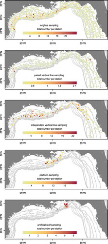
FIGURE 2. Plots of Red Snapper fork length and age frequency based on captures in five different surveys within the northern Gulf of Mexico: bottom longline (LL), vertical line paired with longline (VLpair), independent vertical line (VLind), vertical line on petroleum platform habitat (VLplat), and vertical line on artificial reef habitat (VLart). Solid black lines denote the mean length and age for each survey.

The second survey was conducted from August 27 to September 7, 2007, and deployed VLs on petroleum extraction platforms (VLplat) in the north-central GOM from Alabama to Louisiana (87–92°W). Stations were selected from strata defined by longitude and depth (6–30, 30–75, and 75–152 m) and were proportional to the number of platforms within a given stratum (see the full description of methodology in Moser et al. 2012). Three VLs were fished simultaneously at each site and consisted of 10 circle hooks (size 11/0) per reel. Of the 289 Red Snapper that were captured, 138 were aged using the protocols described by Allman and Fitzhugh (2007), and length measurements only were available for all but three of the remaining individuals. For those individuals with only length observations, ages were assigned based on an age–length key (10-mm length bins) developed from the aged subsample of individuals. The three individuals without age or length data were assigned ages randomly based on probabilities that were proportional to the observed age composition in the survey.

The third survey was conducted from March 21 to September 14, 2011, and deployed VLs on artificial reef structures (VLart) within the Reef Permit Zone in the north-central GOM off the coast of Alabama. Prior to VL sampling, structures were identified and enumerated with side-scan sonar. Stations were then randomly selected from strata defined by depth (18–37, 37–55, and 55–91 m following Gregalis et al. 2012), with effort allocated in proportion to the areal extent of each depth stratum. Two VLs were fished simultaneously at each site; each line consisted of 12 circle hooks of sizes 8/0, 11/0, 13/0, and 15/0 (n = 3 hooks of each size). Complete details are provided by Gregalis et al. (2012). Ages for 20 of the 519 Red Snapper were missing from the database; therefore, the ages of those fish were back-calculated from known lengths by using an age–length key based on the aged sample in the survey. A single individual lacked both length and age information and was assigned an age randomly, as in the CSSP and platform surveys. All other fish were aged in accordance with the methods of Allman and Fitzhugh (2007). Other than the structures targeted by the VLpair, VLind, VLplat, and VLart surveys, the only other difference among surveys was the proportions of different-sized hooks that were used.

Hereafter, we use the term “gear” to model the five gear × survey type combinations described above (LL, VLpair, VLind, VLplat, and VLart); note that while all VL surveys use the same gear, the statistical design of each survey had inference over a different area. By poststratifying the entire northern GOM into the areas where each survey had valid inference, we were able to combine inferences over the entire region. The LL and VLpair surveys were conducted as part of a stratified random sampling design wherein strata were selected based solely upon depth and broad spatial areas, with no consideration of habitat type. Furthermore, due to safety and logistical considerations, LL deployments avoided known wrecks, artificial reefs, and petroleum platforms. Hence, the LL data and VLpair data had inference over the entire sampling domain except for natural reefs, platforms, and artificial reefs. In contrast, the VLind (independent VL on identified rock and gravel structure), VLplat (platforms), and VLart (artificial reef) surveys only had inference over the particular substrate that they sampled.

Habitat Information

Habitat information from the usSEABED database (offshore surficial sediment data; Buczkowski et al. 2006) was used to poststratify the northern GOM into areas of valid inference for each survey and gear type. The usSEABED database is an extensive collection of observations on benthic substrate composition and represents the most comprehensive habitat data source available for the region. A fuzzy logic membership technique was used to categorize historical and recent observations into broad grain types (Buczkowski et al. 2006). We used usSEABED’s 255,562 point estimates of percent rock, gravel, sand, and mud throughout the northern GOM as the basis for our habitat composition estimates. For each grid cell in our 10-km² prediction grid, we calculated the average percent rock, gravel, sand, and mud for the data points falling within that cell. The usSEABED database has a resolution of at least 2 km² in most areas; therefore, most grid cells contained approximately 25 point estimates of habitat cover. When no usSEABED estimates were available (only 3 of 2,581 grid cells), an average from the eight surrounding grid cells was used. The resulting output was a measure of percentage composition for each prediction grid cell (Figure 3).

FIGURE 3. Distribution of natural habitats and artificial structures throughout the prediction domain within the northern Gulf of Mexico, as defined by the databases used in this study. Percent artificial structure influence is calculated based on the number of structures (petroleum platforms and artificial reefs) in each prediction cell multiplied by the area of assumed influence (a 100-m radius; AARZ = Alabama Artificial Reef Zone).

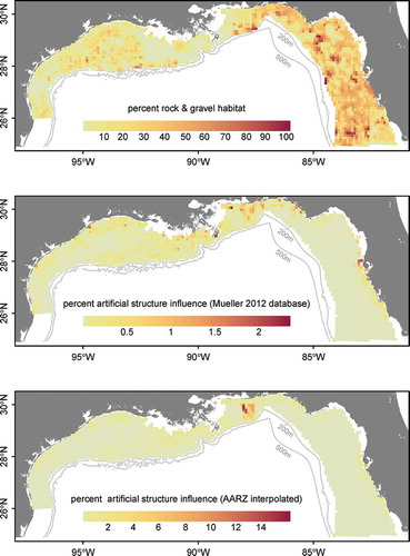
Petroleum platform locations were taken from the Platform Structures Database (Bureau of Ocean Energy Management; www.data.boem.gov/itaccessproj/platformstructures.mdb; accessed December 2015). The database included 7,121 total structures, 4,713 of which were marked as “removed” (i.e., clear of any structure or trash) and thus were not included in the analysis. Of the remaining 2,408 platforms, 2,014 fell within our statistical study domain. Locations of artificial structures were derived from the data sources described by Mueller (2012). Artificial reef structures included both shipwrecks or obstructions and state-permitted artificial reefs (including oil rigs that had been converted to reefs) and comprised a total of 3,689 structures within the prediction domain. In the Alabama Artificial Reef Zone (AARZ), which encompasses approximately 2% of the total prediction domain, the numbers of artificial reefs were updated based on a side-scan sonar survey. For this survey, the AARZ was divided into a series of 2-km² grids prior to sampling. Between 2011 and 2014, 60 grids were randomly selected and surveyed with side-scan sonar. Surveyed structures within the grids were classified either as (1) qualifying as an artificial reef structure (area > 4 m²; vertical relief > 0.5 m²) or (2) nonqualifying (area < 4 m², vertical relief < 0.5 m²; Gregalis et al. 2012). After categorization, the qualifying structures within each of the surveyed grids were identified and enumerated to calculate an artificial reef density (artificial reefs/km²) for each surveyed grid. Artificial reef densities were then interpolated from the side-scan sonar surveyed grids by using the Empirical Bayesian Kriging Interpolation tool in ArcGIS version 10.2. These interpolated densities (summing to 7,266 artificial structures in the AARZ) were then used in lieu of the artificial reef density estimates from the Mueller (2012) database (which contained only 673 artificial structures in the AARZ; Figure 3). Because this difference could imply that the Mueller (2012) database similarly underestimated the numbers of artificial reefs in areas outside of the AARZ, we carried out a sensitivity analysis wherein the numbers of artificial reefs were quadrupled for each grid cell outside the AARZ, giving a total of 19,330 artificial reefs in our statistical domain compared to 10,282 artificial reefs in the baseline case. The sensitivity analysis allowed us to understand how our final results could be affected by a potentially gross underestimate of the number of artificial reefs.

Statistical Modeling Approach

Below, we present a detailed explanation of our statistical approach; a flowchart is included for a conceptual representation (Supplementary Figure S.1 available separately online with this article). The index of Red Snapper relative abundance at grid cell i was calculated as a weighted average of relative abundances on natural habitat and artificial structures,

(1)

where NAT is the relative abundance on natural habitat (given by equation 2); PLAT is the relative abundance on platforms (calculated from equation 13); ART is the relative abundance on artificial reefs (calculated from equation 14); and %PLATarea and %ARTarea are the percentages of the 10-km² grid cell i covered by platforms and artificial reefs, respectively (Figure 3). The area is calculated by multiplying the number of artificial structures in each 10-km² grid cell by π·0.1² km², as the high fish densities found on platforms have been shown to extend approximately 100 m from the platform center (Reynolds 2015).

The relative abundance on natural habitats within each 10-km² grid cell i was calculated as

(2)

where

(3)

a represents different age-classes; VLpair and VLind are standardized relative abundances calculated for the paired VL and independent VL gear, respectively (from equations 6 and 7); %mud, %sand, %rock, and %gravel are estimates of the percent habitat type in each 10-km² grid cell; and F_a,r is an age adjustment factor that accounts for the fact that no gear selects 100% of the fish in each of the age-classes (see equation 8).

Calculation of NAT_i

Estimates of relative abundance on the different habitat types in each sample site d were calculated for the VLpair and VLind surveys by modeling the effects of gear and other sampling artifacts in a two-stage approach. The two-stage approach was used due to the zero-inflated nature of the data set; only about 6% of the observations had one or more individuals present. The presence–absence (p) of six age-classes was modeled with logistic regression and as a function of age, gear type, the month and hour of sampling, and the longitude and depth at which sampling was conducted,

(4)

Abundance when present was modeled as a Poisson regression using the following link function:

(5)

Gears included in the model were LL, VLpair, and VLind. Note that although the LL gear was included in the model because it was informative for helping the model estimate effect sizes for each factor as well as the VL gear’s selectivity at age, the relative abundance estimates produced from LL gear were not used in subsequent calculations. Those estimates could not be used because the “gear effect” estimated for the LL gear contained the confounding effects of (1) differences in abundance due to habitat type and (2) differences in catchability due to the nature of the gear. Because the gears used in the VLpair and VLind surveys were identical in every aspect except the habitat they sampled, they could be used in reference to each other to estimate the relative abundances on the different habitat types; in other words, the gear effects estimated by the model for the VL gears contained only habitat effects.

All other variables included in the generalized linear models (GLMs) were treated as categorical factors; longitude (from 98°W to 81°W) was binned at 1.5° or 2.0° resolution, depth (7–140 m) was categorized into 10-m bins, and time (all 24 h) was assigned to 6-h bins. Variables were checked for the presence of collinearity; none of the pairs had a correlation coefficient (r) greater than 0.20. To attain model convergence, age-classes were limited to those ages observed by all gears; thus, age-1 and age-2 individuals were combined into a single age-class, and age-7 and older individuals were combined into the oldest age-class. Age × gear interaction effects were modeled because catchability rates for both gears appeared to be largely dependent on fish size, and age × depth interactions were included because of the well-documented ontogenetic movement of Red Snapper from shallow to deep waters (Mitchell et al. 2004). Age × month and age × hour interaction effects were also included in candidate models. We considered several rugosity measures based on the 30-arc-second-resolution bathymetry data from the General Bathymetric Chart of the Oceans (www.gebco.net); however, rugosity was highly correlated with depth (r > 0.70) and therefore was not ideal for inclusion. Instead, we included a depth × longitude interaction factor, which allowed for the depth effect to differ by area. In modeling the positive count data, we considered both Poisson and negative binomial regression. Decisions on which factors to include in the model and on the form of the regression were initially made based on Akaike’s information criterion (AIC). Models with similar AIC scores were subjected to further model performance testing based on a 10-fold cross-validation procedure. In this procedure, the full data set was randomly split into 10 groups, and each group served once as a validation data set while the other nine groups were used as a model training set. Model performance was evaluated by (1) estimating the model on the training data set, (2) using the model to predict data points in the validation set, and (3) measuring the agreement between the observed validation set and the predicted values via Pearson’s product-moment correlation coefficient. The two-stage logistic–Poisson regression model containing the full suite of individual factors and three interaction effects (as described above) had the best performance, and the outputs were selected for further calculations.

For the purposes of model prediction, a regular 10-km² grid was overlaid on the study domain; the domain was defined by the isobaths between which Red Snapper were actually observed during the surveys (i.e., from 7- to 140-m depth). To estimate the total biomass across the domain, we first extracted the longitude and depth at which each of the center grid points fell. Using the parameter estimates from the logistic model (equation 4) and Poisson model (equation 5) that were built previously (Table 1), we then predicted, for each grid cell, the expected probability of occurrence (p) and positive counts (number present [NP]). The expected quantities were calculated separately for VLpair and VLind and for each Red Snapper age-class based on the given longitude and depth bins and based on the average month and hour effects. Multiplying p by NP then yielded the relative abundance expected for each gear type across the study domain in the absence of sampling artifacts,

(6)

TABLE 1. Percent deviance explained by each factor in the logistic model of the probability of presence and the Poisson model of positive counts (i.e., abundance when present) for Red Snapper in the northern Gulf of Mexico.

Factor	df	Deviance	Residual df	Residual deviance	Deviance explained (%)
Logistic model (probability of presence)
Null			18,617	8,223.7
Age-class	5	230.3	18,612	7,993.4	2.80
Gear	2	766.0	18,610	7,227.4	9.58
Depth	6	229.1	18,604	6,998.3	3.17
Longitude	7	310.4	18,597	6,687.9	4.44
Month	6	59.3	18,591	6,628.6	0.89
Hour	3	14.3	18,588	6,614.3	0.22
Age-class × gear	10	193.7	18,578	6,420.6	2.93
Age-class × depth	30	117.3	18,548	6,303.3	1.83
Depth × longitude	42	235.5	18,506	6,067.8	3.74
Poisson model (abundance when present)
Null			1,082	1,469.8
Age-class	5	32.48	1,077	1,437.4	2.21
Gear	2	0.22	1,075	1,437.2	0.02
Depth	6	28.42	1,069	1,408.7	1.98
Longitude	7	35.61	1,062	1,373.1	2.53
Month	6	48.10	1,056	1,325	3.50
Hour	3	1.91	1,053	1,323.1	0.14
Age-class × gear	10	59.54	1,043	1,263.6	4.50
Age-class × depth	30	91.54	1,013	1,172	7.24
Depth × longitude	42	63.23	971	1,108.8	5.40

and

(7)

The relative abundance of Red Snapper on natural habitat in each grid cell i was then calculated as a weighted average of the abundance estimated by each gear type times the percent cover in the grid cell of the habitat over which each gear type had inference (equation 3). This final estimate of relative abundance was then multiplied by the factor F_a,r (equation 2), which accounted for the fact that due largely to size selectivity, neither the VL gear nor the LL gear sampled the younger age-classes as efficiently as the older age-classes; thus, the model predicted that age-3 and age-4 fish were more abundant than age-1 and age-2 fish. Abundance at age was extracted from estimates from the most recent stock assessment (Cass-Calay et al. 2015), and the multiplicative factor was calculated as

(8)

where S_a,r is the abundance-at-age-a vector by region r in 2011, as estimated from the stock assessment; and N_a,i is the total relative abundance at age calculated by the weighted model as above (equation 3). Region r is defined as either east or west, with a cutoff at approximately the Mississippi–Louisiana border (–89.1°W), as is used in the assessment. Application of the multiplicative factor adjustment did not change the patterns in spatial distribution by age, as it was a constant applied across all grid cells. However, the adjustment was necessary to ensure that the spatial distribution of the summed age-classes was driven by the spatial distributions of the youngest age-class rather than the older age-classes—thus emulating reality, wherein abundance decreases with age due to natural mortality. It was also necessary to make the multiplicative factor region-specific to account for the fact that the binned age-classes (ages 1–2 and ages 7+) contained different age compositions in each region; most notably, the eastern region had substantial age truncation relative to the western region. Note that this scaling was done only to correct for selectivity but not to scale to the actual abundance estimates produced by the assessment; the abundance index produced by our method is relative.

Calculation of PLAT_i and ART_i

The relative abundance of Red Snapper on artificial structures was calculated via a comparison of VL sampling on natural reefs, platforms, and artificial reefs. Because the same gear and sampling methodology were used in all three surveys, any differences in catch rate are presumably due only to differences in relative abundance on the various habitat types (i.e., natural habitat with structure; petroleum platforms; or artificial reefs). For the comparison, the same two-stage modeling procedure was employed as described above (similar to equations 4 and 5), except that because the three surveys differed slightly in the arrangement of the various hook sizes, an additional age × hook size interaction term was included (the depth × longitude interaction factor was excluded due to nonconvergence):

(9)

and

(10)

Because the same gear was used across different habitat types, this approach produced estimates of the “habitat effect” after accounting for differences in other sampling artifacts. The model coefficients from equations (9) and (10) were then used to predict back onto all combinations of depth bin, longitude bin, month, hour bin, and hook size for each gear type and age-class. Average relative abundances for each gear type were averaged over the individual depth bins and age-classes. This calculation represents, for each depth and age-class, the relative estimates of Red Snapper abundance on platforms, artificial reefs, and natural reefs without the effects of sampling artifacts. Ratios of abundance (platforms : natural reefs; artificial reefs : natural reefs) were then calculated based on the mean estimated abundances (, , and ; see Table 2). Because the platform sampling was carried out in 2007 and all other sampling was conducted in 2011, the ratio also had to account for the differences in numbers at age between the two time periods, as estimated from the most recent stock assessment (Cass-Calay et al. 2015),

(11)

TABLE 2. Ratio of average catch rates of Red Snapper on petroleum platform habitats or artificial reefs versus targeted natural habitats in the northern Gulf of Mexico, presented for each age-class and depth bin.

	Depth (m)
Age	0–40	40–50	50–60	60–70	70–80	80–90	>90
Platforms : natural habitats
1–2	18.72	16.41	21.56	23.99	24.81	25.12	26.11
3	3.66	3.48	4.04	4.14	4.28	4.42	4.51
4	0.43	0.43	0.43	0.43	0.43	0.43	0.43
5+	0.18	0.18	0.19	0.19	0.20	0.20	0.19
Artificial reefs : natural habitats
1–2	20.07	19.50	19.83	20.62	19.10	19.82	20.45
3	8.93	8.87	9.05	9.11	8.87	8.90	8.96
4	16.38	17.18	17.16	16.29	16.26	17.30	17.69
5+	18.40	18.04	18.67	17.46	17.58	19.59	17.65

Sampling on both artificial reefs and natural reefs was carried out in 2011, and thus the calculation of the ratio was straightforward:

(12)

The average relative abundance indices and subsequent ratios were not calculated over individual longitude bins because the artificial structure data were available for only a small spatial extent: mostly off the coast of Louisiana for platforms and only the AARZ for artificial reefs (see Figure 1). Thus, the predictions of the relative abundance differences between platforms and natural habitats were extended beyond the area upon which the predictions were based. The present results regarding relative abundances on artificial structures should therefore be treated with caution since they serve only as best available estimates of artificial structures’ influence on distributions in the absence of more extensive sampling at those habitats.

The relative abundances of Red Snapper on platforms and artificial structures in each grid cell i (PLAT_i and ART_i in equation 1) were calculated as

(13)

and

(14)

where VLind_a,i is as calculated in equation (7), PLATFORM : NATURAL_a,i is the ratio of abundances between platform and natural habitats as calculated in equation (11), ARTIFICIAL : NATURAL_a,i is the ratio of abundances between artificial reef and natural habitats as calculated in equation (12), and F_a,r is the relative-abundance-at-age multiplicative factor as described in equation (8). The quantities PLAT_i and ART_i were then used in equation (1) for the final calculation of Red Snapper relative abundance in each grid cell.

Calculation of variance estimates

Variances for the combined logistic presence–absence and Poisson counts were calculated by using Goodman’s exact estimator, as recommended by Lauretta et al. (2015),

(15)

Variances of the combined prediction from the VLpair and VLind gears over all natural habitat types were calculated using the weighted variance formula,

(16)

Total variances were then scaled by the square of F_a,r and its associated variance, var(F_a,r), as estimated from 500 bootstrap estimates of the region-specific abundance-at-age matrix from the stock assessment model. The variance was summed across age-classes to calculate the total variance from the GLM for each grid cell i,

(17)

We additionally employed a nonparametric bootstrapping method to estimate variances of the GLMs, as those estimates may differ from the analytical approximation when model fit is poor or when overdispersion occurs. We calculated bootstrapped variances by resampling the original data, refitting the GLMs, and then calculating the SD of the bootstrapped parameter estimates. We found that the nonparametric estimates of variance were very similar to the derived estimates; thus, we kept the analytical approximations for our calculations.

Calculation of the biomass index and fecundity index

Relative biomass and relative fecundity were estimated concurrently with relative abundance within the same framework. Because all model calculations were performed on an age-class-explicit basis, conversions to biomass and batch fecundity were made simply by introducing a multi-plicative weight-at-age or fecundity-at-age vector term. Those terms were included in equations (2), (13), and (14), where weight at age or fecundity at age was multiplied by F_a,r to convert to biomass or egg numbers, respectively. Weight-at-age estimates were based on growth equations reported in the most recent stock assessment (Cass-Calay et al. 2015); the fecundity-at-age relationship we used was from Porch et al. (2015).

Evaluation of spatial autocorrelation in residuals

The modeling approach presented in equations (2)–(8) represents the expected relative abundance in each grid cell based on its habitat composition, depth, and longitude (i.e., the quantity NAT_i). The quantity does not account for habitat differences that occur on scales finer than those at which the sampling took place, and the predictions obtained from equations (4) and (5) still have substantial unexplained deviance. To evaluate the subsample-scale variation in abundance, we carried out kriging of the spatially explicit model residuals. The residual abundance at a data point d was calculated as a percentage,

(18)

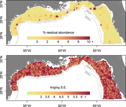
where N_a,d,observed is the raw observed abundance at each data point; and N_a,d,expected is the predicted abundance at age at each data point. The expected values were calculated based on the coefficients from the models fitted in equations (4) and (5), which were used to predict back onto the original data points based on their given gear, depth, longitude, month, and hour of sampling. The quantity %ε_d thus represents the percent residual abundance at the site that was not accounted for after standardization across all factors. The small-scale residual variation in abundance was interpolated across the study domain via kriging. An empirical variogram was estimated for data pairs with distances less than 50 km by using the classical method-of-moments estimator. The variogram model was fitted by using ordinary least squares, with no fixed nugget (Figure 4). Variograms based on residuals from data points that were sampled by VL gear showed poor fits; the sample sizes were likely too low to permit detection of spatial autocorrelation. However, we do present the residuals based on LL data points because they produced a good fit to the variogram. Parameters from the LL-only variogram model were then used to generate predictions of residual abundance across the 10-km² prediction grid to represent unexplained patterns in relative abundance.

FIGURE 4. Variogram model fit used for kriging the residuals of bottom longline data set predictions from the generalized linear model of Red Snapper relative abundance.

RESULTS

Catch

Overall, 2,485 Red Snapper were caught during the CSSP survey: fish that were caught on LL gear ranged from 280 to 885 mm FL (n = 776), and those caught on the VLpair and VLind gear ranged from 154 to 782 mm FL (n = 1,709). The VLplat survey captured 289 Red Snapper ranging from 258 to 552 mm FL, while the VLart survey captured 519 individuals ranging from 235 to 855 mm FL. Larger fish were captured on the LL gear than on any of the VL combinations (VLpair, VLind, VLplat, and VLart; Figure 2). Ages from the CSSP survey ranged from 2 to 34 years on LL gear and from 1 to 22 years on VLpair and VLind. The VLplat survey captured Red Snapper ranging in age from 1 to 7 years, while the VLart survey captured fish of ages 1–12. The LL survey captured the oldest Red Snapper, on average, whereas the VLplat survey captured the youngest individuals. The VLpair, VLind, and VLart surveys all captured similarly aged Red Snapper.

Statistical Modeling

For the estimates of Red Snapper relative abundance on natural habitat by sample site, the best model based on cross validation for both logistic presence–absence (equation 4) and Poisson positive counts (equation 5) contained all factors, including the age × gear type, age × depth, and depth × longitude interactions. The addition of other interaction factors (age × month, age × hour, or both) led to slightly decreased performance in the cross validation when included in either the presence–absence model or the positive count model and thus were excluded. Cross validation for the best-performing pair of models showed an r of 0.36 for observed versus predicted values. When the depth × longitude interaction term was dropped, the r-value was reduced to 0.33; when the age × depth term was dropped, the r-value was reduced to 0.30; and when no interaction factors were included, the r-value was 0.25. Poisson regression outperformed negative binomial regression; furthermore, the full model with three interaction terms would not converge for the negative binomial formulation of the regression. For the logistic model, 26.2% of model deviance was explained, and the Poisson model for positive counts explained 24.6% of the deviance (Table 1). Variograms estimated at a maximum distance of 50 km (Figure 4) showed good fits for the subset of LL data only, and high spatial autocorrelation was estimated for distances of up to about 10 km (Figures 4, 5). Kriging error was relatively high compared to the total regression model error, indicating substantial residual variation.

FIGURE 5. Kriged predictions of the residual abundance and associated SEs for Red Snapper in the northern Gulf of Mexico.

Distribution Patterns

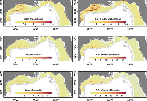
Spatial distribution patterns of Red Snapper were generally estimated to be highest in the middepth ranges off the coast of Texas and in shallow-water “hot spots” within the north-central and northeastern GOM (Figure 6). In particular, high densities were estimated for areas just off the coast of Alabama and the Florida panhandle region. Similar patterns were estimated for biomass and fecundity distributions across the domain; higher numbers occurred in the northwestern GOM and off the coast of Louisiana. Biomass and fecundity estimates were lower on the west Florida shelf and off the coasts of Alabama and Florida, indicating the presence of younger individuals that contributed relatively less to biomass and fecundity (Figure 6). The fecundity index was estimated to be highest off the coast of Texas, particularly in middepth waters (50–90 m) and, to a lesser extent, off the Louisiana coast (Figure 6).

FIGURE 6. Maps of relative abundance, biomass, and fecundity (with associated SEs; see Methods) for Red Snapper in the northern Gulf of Mexico based on the generalized linear model.

Influence of Artificial Structures

Catch rates of Red Snapper on artificial structures were much higher than those on natural reefs (Table 2). Platforms had the highest catch rates for 1- and 2-year-old fish, particularly in the over 50-m depth range, where the average catch rate on platforms was estimated to be up to 26 times the catch rate on natural reefs. This ratio decreased with age, and for 4- and 5-year-old fish, the platform catch rates were actually less than the natural reef catch rates. For artificial reefs, catch rates of 1- and 2-year-old Red Snapper were estimated to be about 20 times the catch rates on natural reefs across all depth bins. In contrast to the results for platforms, higher catch rates on artificial reefs relative to natural reefs were maintained for the older age-classes: age-5 and older individuals had artificial reef catch rates that were around 18 times the natural reef catch rates.

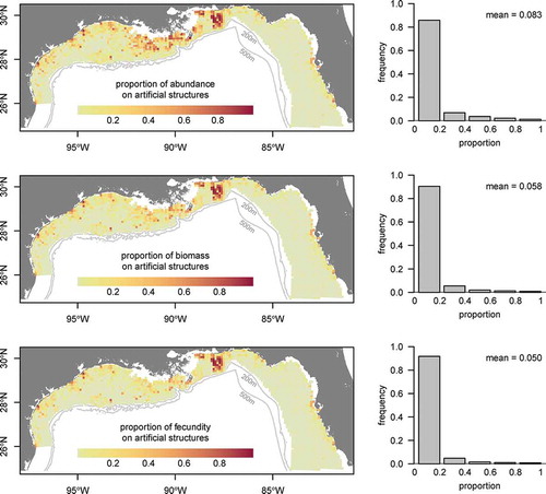
The inclusion of artificial structures had a notable effect on the distribution, biomass, and fecundity maps due to the high catch rates observed on those structures (Figure 7). We estimated that 13.3% (by number) of the northern GOM population of Red Snapper was present on artificial structures (Table 3; Figure 8). Because artificial structures attracted younger age-classes of Red Snapper, estimates of biomass and fecundity on artificial structures were lower—about 7.8% and 6.4%, respectively (Table 3). Among 1–2-year-olds, 15.9% of individuals were estimated to occur on artificial structures, 3.3% were estimated to occur on platforms, and 12.6% were estimated to occur on artificial reefs (Table 4). These percentages declined for older age-classes, and less than 5% of age-7 and older individuals occurred on artificial structures (Table 4). Estimated numerical, biomass, and fecundity contributions were relatively robust to high uncertainty around the actual number of artificial structures (Table 3).

TABLE 3. Total contribution of natural habitats and artificial structures to the Gulf of Mexico Red Snapper population in terms of number, biomass, and fecundity (see Methods). Values in parentheses are results from the sensitivity analysis representing uncertainty in the number of artificial reefs.

Habitat type	% Number	% Biomass	% Fecundity
Natural
All natural	86.72 (77.14)	92.22 (84.55)	93.65 (86.23)
Sand and mud	14.47 (12.87)	19.88 (18.22)	21.35 (19.66)
Rock and gravel	72.25 (64.27)	72.34 (66.33)	72.3 (66.57)
Artificial structures
All artificial	13.28 (22.86)	7.79 (15.46)	6.35 (13.78)
Platforms	2.31 (2.05)	0.44 (0.40)	0.11 (0.10)
Reefs	10.97 (20.80)	7.35 (15.06)	6.24 (13.68)

TABLE 4. Percentage of individuals from each Red Snapper age-class that were estimated to occur on natural habitats or artificial structures, calculated across the entire northern Gulf of Mexico.

Habitat type	Ages 1–2	Age 3	Age 4	Age 5	Age 6	Age 7+
Natural
All natural	84.10	92.71	89.53	91.27	93.79	95.23
Sand and mud	12.30	13.92	14.11	24.64	27.40	20.24
Rock and gravel	71.80	78.80	75.42	66.64	66.39	74.99
Artificial structures
All artificial	15.90	7.29	10.47	8.73	6.21	4.77
Platforms	3.31	0.56	0.06	0.02	0.02	0.03
Reefs	12.59	6.73	10.41	8.71	6.19	4.74

FIGURE 7. Maps of predicted relative abundance, biomass, and fecundity (see Methods) for Red Snapper in the northern Gulf of Mexico based on the generalized linear model and abundance estimates for artificial structures.

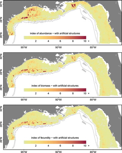
FIGURE 8. Maps of the proportion of Red Snapper relative abundance, biomass, and fecundity occurring on artificial structures in the northern Gulf of Mexico. Histograms show the distribution of the data points in each map.

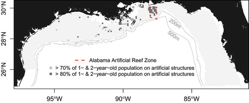
In some locations, particularly off the coast of Louisiana (where platform densities can be almost 1 platform/km²), platforms harbored substantial numerical abundances of Red Snapper. Because natural habitat is limited along the shallow Louisiana coast, platforms can provide the majority of structure for age-1 and age-2 Red Snapper (Figure 9). The AARZ also contributed substantially to the abundance of Red Snapper, attracting not only young fish but also high numbers of 3-, 4-, and 5-year-olds. Note that platform sampling was not carried out across the entire area where platforms occurred, and artificial reef sampling was restricted to the small area of the AARZ. Thus, areas outside the sampling zone were extrapolated with the assumption that the ratios of catch rates on platforms and artificial reefs relative to natural reefs were the same as the ratios in the sampled areas.

FIGURE 9. Influence of artificial structures on age-1 and age-2 Red Snapper abundance in the northern Gulf of Mexico. Grid cells highlight areas where at least 70% or 80% of the age-class is estimated to occur on artificial structures.

DISCUSSION

Our modeling approach was able to predict Red Snapper spatial distribution by age based on broad metrics, such as longitude and depth, while accounting for differential catchability with different gears. Gear type was one of the more influential variables in the statistical model for the probability of presence, reflecting the complexity of surveying reef-associated fish with differential vulnerability based on gear type, habitat, or ontogeny. Estimation of the gear effect by age allowed for survey gears with differential selectivity to be combined into a consistent estimator. Clearly for Red Snapper and likely for other reef-associated species, maps of relative abundance based upon a single gear type miss large components of the stock and may not reflect the spatial distribution of the stock as a whole. Other important factors in the model were longitude and depth, indicating a general westward cline in relative abundance and differential depth utilization over ontogeny. The age × depth interaction (i.e., older ages occurred more frequently in deeper waters) reflected the ontogenetic shifts displayed by the species (Gallaway et al. 2009; Ajemian et al. 2015). In general, the model results highlighted the importance of accounting for age and size selectivity when making population-level inferences.

Our modeling approach explicitly reveals the spatial precision of the maps—a measure that unfortunately is rarely reported in spatial mapping studies based upon predictive models. We feel that any spatial map should be accompanied by estimates of precision, without which the reliability of the model predictions cannot be evaluated. As model-based estimates, variance estimates from the GLM derive their utility and unbiasedness from the degree to which the underlying models and assumptions thereof are correct (Cassel et al. 1977). Generalized linear models generally assume that the data are representative of the population. Because there was no existing comprehensive survey of platforms and artificial reefs in the GOM, it was necessary for us to assume that the sampled artificial structures were representative of the entire population of artificial structures in the GOM—a caveat that was noted above. Greater sampling of these structures outside of the northern GOM could address this assumption. Generalized linear models further assume that the data are independent and identically distributed; in this case, given the opportunistic sampling of the CSSP, true independence of the data was unlikely. The practical implications of a lack of independence would be that the variances likely represent underestimates of the true variance. Note that the results of the logistic model indicated the presence of underdispersion, which also suggests that variation in the data is less than would be predicted under the model assumptions. Hence, the spatial variances are likely to be underestimates of the true variability one might find in repeated observations at the same location; however, they are useful for providing an indication of the model’s reliability over the prediction space. Overall, the maps showed relatively high spatial precision except in certain areas of the west Texas shelf, from which few samples were available.

As an additional measure of the adequacy of our predictive modeling, we calculated the spatial autocorrelation of the residuals and plotted interpolated estimates of the residual abundance. Autocorrelation was present only for the residuals of the LL predictions, and evidence of residual hot spots indicated that the models missed some spatial structure at scales of 30 km or less. This indicates the occurrence of spatial patchiness that was unaccounted for by the model at scales slightly coarser than the 10-km² resolution of the predictions. Such residual variation could be due to the fact that (1) the samples used in modeling may not be entirely independent or (2) Red Snapper respond to finer-resolution habitat characteristics than are captured by the resolution of available habitat data, a common issue in the marine realm (Lecours et al. 2015). In a previous study of GOM snappers and groupers, Saul et al. (2013) reported that spatial autocorrelation of species abundances occurred at scales less than 1 km and that patches of habitat were autocorrelated at ranges between 1 and 6 km (Saul et al. 2013); those scales are much finer than the resolution of our predictions. Furthermore, Saul et al. (2013) could not detect spatial autocorrelation in Red Snapper, even at the fine scales they examined. Residuals of the model predictions from our full data set did not display spatial autocorrelation, likely because the sampling was carried out at scales larger than those relevant to the habitat.

One limitation of our predictions was the low amount of overall variance explained by the GLMs, which begs the question of whether habitat factors could have been better incorporated into the model. First, habitat type was already accounted for in the sampling design, as several of the surveys occurred on known (and ground-truthed) hard substrate (VLind), platform habitat (VLplat), or artificial habitat (VLart); hence, they only had inference over those areas. Second, although the resolution of interpolated sediment databases (e.g., usSEABED; Buczkowski et al. 2006) is excellent for defining broad habitat metrics and for survey design and stratification, it is of limited utility for identifying the exact spatial locations of reef fish habitat. Because many hard-bottom reefs can be quite small, there is a high potential for mismatch between a fishing location and the habitat predicted by the coarse usSEABED database. A coral reef situated in the middle of a wide sandy area could harbor many reef fish but could easily be classified as “sand” according to the usSEABED database. Previous studies that have assigned interpolated habitat type have had predictive success ranging from “high” for a trawl survey (Drexler and Ainsworth 2013) to “limited” for reef fish sampling (Farmer and Karnauskas 2013). This variable success was likely a function of the relatively coarse resolution of the usSEABED database and the differences in how a trawl survey integrates over a wide spatial area, whereas a handline or trap samples a very specific location. Identification of higher-resolution habitat features (e.g., rugosity, slope, or benthic species composition) could be derived from ongoing side-scan sonar or multiple-beam sonar mapping efforts (e.g., Gledhill et al. 1996) and may improve the capacity for predicting reef fish abundance. However, multiple-beam sonar mapping surveys are relatively costly and limited in spatial extent (Lecours et al. 2015), thus preventing prediction across the entire GOM.

Despite the predictive capabilities of our combined approach, several limitations remain. First, the approach can produce only relative abundances that are scaled to the maximum catchability for any gear type by age-class. Second, there are limitations regarding the comparison of petroleum platforms to natural habitats, particularly in relation to several critical assumptions that rely upon published values in the literature. For example, we used the platform area of influence as estimated by Reynolds (2015) to define the spatial extent of a platform, but we note that any increase or decrease in this estimate would change the resulting percent contribution of platforms. Furthermore, although survey methodologies were consistent between platforms and natural habitats, the surveys were carried out in different years. Adjusting for this difference necessitated the use of age-specific abundances that were derived from the most recent stock assessment as a “bridge” across years. Furthermore, we had to assume that for a given gear type, (1) effort was proportional to abundance and (2) catchability did not differ between habitats. As experimental estimates of differential catchability of the same gear in different habitat types become available (Bacheler et al. 2014), they could be incorporated into the modeling framework we have proposed, perhaps as Bayesian priors. The addition of other paired gears to the survey design (e.g., cameras) could provide further information on catchability or detection rates for the different gears. Finally, the platform sampling and artificial reef sampling were carried out only over a limited spatial domain, and we had to extrapolate the abundance ratios beyond the domain of sampling. We assumed that the abundance ratios PLATFORM : NATURAL and ARTIFICIAL : NATURAL differed based on Red Snapper age and depth but necessarily remained constant across longitudes.

The numbers reported here represent our best estimates based on the most updated literature and available data sets; however, the spatial distribution of the Red Snapper stock will likely change as the population ages and exhibits concomitant ontogenetic movements, as natural mortality and spatial fishing mortality deplete the population, and as other population processes take place. Additionally, we note that presence of anthropogenic material in the marine environment is a dynamic process, as material is deposited by storms, from vessel debris, and via stakeholders’ attempts to improve fishing opportunities. Conversely, material is removed by degradation and sedimentation. Our static sensitivity analysis, in which the distribution with respect to depth and location was kept constant, indicates a direct response to increasing the number of artificial structures—that is, doubling the number of artificial structures approximately doubles the number of fish that inhabit artificial structures. However, the actual population-level response is unknown and is unlikely to be linear, as destruction or removal may take place across different depth strata or geographical locations over time. Furthermore, due to density-dependent effects, the relationship between the number of artificial structures in an area and the abundance of Red Snapper may also be nonlinear (Campbell et al. 2011). Note that with the appropriate survey—for example, simultaneous sampling of natural habitats versus artificial structures in areas of varying densities, across a range of depths and longitudes, and with a comprehensive mapping of habitats—our model could be updated, obviating some of the strong assumptions that were necessary in this analysis.

Contribution of Artificial Structures

Previous estimates of platform contributions based on observations of oil rig explosions have suggested that platforms hold the majority (70–80%) of age-2 Red Snapper in the GOM (Gallaway et al. 2009). In contrast, we estimated that platforms currently hold substantially fewer (~3.3%) 1- and 2-year-old Red Snapper. These discrepancies can be explained largely by the fact that Gallaway et al. (2009) derived the fraction of Red Snapper on oil rigs by dividing the assumed population of Red Snapper at the time. Gallaway et al. (2009) used population size estimates from an earlier stock assessment (SEDAR 2005) that reported substantially lower natural mortality rates for ages 1 and 2 (0.6 and 0.1 year^–1, respectively; SEDAR 2005) compared to values from the current assessment (1.6 and 0.7 year^–1, respectively; SEDAR 2013). In subsequent years, estimates of natural mortality for young Red Snapper were revised upward based on studies indicating that natural mortality is likely higher than previously assumed (Gazey et al. 2008). Consequently, the total number of age-1 and age-2 fish estimated to be present in the early 1990s at the time Gallaway et al. (2009) made their calculations is now estimated to be substantially higher to support the same number of removals. The most recent estimates of 1- and 2-year-old Red Snapper abundance in only the western GOM at the beginning of the year in 1992 are approximately 30.0 and 4.3 million fish, respectively (SEDAR 2013). Using the same logic as Gallaway et al. (2009) and based on the numbers from Gitschlag et al. (2003), we would estimate a substantially lower fraction (7–25%) of age-1 and age-2 Red Snapper on platforms. We note that the number of platforms has declined as older ones are removed or repurposed; the estimates are approximately 2,000 platforms in 2011 versus 4,000 platforms in 1992. If we apply our calculations to the number of extant platforms in 1992 while assuming that all other factors were relatively constant (e.g., depth, platform locations, and the ratio of catch rates between the areas), the fraction of the Red Snapper population occurring on platforms would double to approximately 7%.

Our findings confirm other notions regarding habitat usage by Red Snapper in the GOM. First, our statistical model estimated that age-1 and age-2 Red Snapper preferentially inhabit high-relief structures, both natural and artificial, and that the preference for deeper, less-structured habitats increases with age, which is consistent with the current body of knowledge (Gallaway et al. 2009). Our calculations also show that in comparison with natural habitats, artificial structures indeed harbor greater densities of Red Snapper: in deeper waters, the abundance of 1–2-year-olds at artificial structures was up to 26 times the abundance in natural habitats. Other authors have highlighted that a large portion of Red Snapper landings comes from artificial reefs in some parts of the GOM (Gallaway et al. 2009; Shipp and Bortone 2009), and our distribution maps would suggest that this is accurate for some localized areas, particularly the AARZ, where artificial structures are estimated to contain approximately 80% of the total Red Snapper biomass. However, given the low fraction of the population associated with artificial structures overall, the potential for population-level impacts (either positive or negative) from artificial structures is relatively low. Recent studies have suggested that Red Snapper living on platforms possess lower reproductive potential than Red Snapper on natural habitats (Glenn 2014; Schwartzkopf 2014), which could be linked to differential diet characteristics (Simonsen et al. 2014). However, given the small influence of platforms in supporting spawning biomass (a mere 0.11% of the total), it is unlikely that lowered reproductive potential on platform habitats would markedly alter population dynamics.

Platform structures in particular may harbor greater abundances per unit of sea floor because they provide more three-dimensional habitat space on a given footprint of the sea floor (Martin and Lowe 2010). However, unlike the apparent situation in the study by Claisse et al. (2014), wherein platforms appeared to increase the actual level of fish production, the production versus attraction debate is still unresolved for GOM Red Snapper. The analyses presented here provide only static estimates of Red Snapper relative abundance on various natural habitats and artificial structures; however, they do not lend insights into the relative productivity of different sectors of the population, and we cannot speculate upon the dynamic response of the population to increases or decreases in artificial structures. We found that artificial structures harbored substantial numbers of young Red Snapper, particularly in areas with high densities of artificial structures and little natural reef habitat. Indeed, in those areas, artificial structures harbored the majority of the 1–2-year-old fish. However, when calculated across the entire GOM—much of which is devoid of artificial reefs and platforms—artificial structures make up only a small proportion of the total available habitat. Additionally, although the contribution of artificial structures was relatively large for young Red Snapper, their importance decreased for older age-classes. Therefore, in terms of biomass and fecundity, the influence of artificial structures was minimal, as they harbored just over 6% of the total spawning potential for the GOM Red Snapper population.

Conclusions

One of the greatest challenges to assessment and management of marine resources is the effective incorporation of spatial processes. The current assessment of Red Snapper (SEDAR 2013) uses a coarse, two-area model that divides the population at the mouth of the Mississippi River. However, stakeholders are increasingly calling for finer-scale spatial management, and there is a growing recognition of the importance of spatial and habitat type variability in key biological parameters (Glenn 2014; Schwartzkopf 2014; Simonsen et al. 2014) and very likely in fishing mortality and removals. Developing a spatial map of the population, such as that presented here, represents a critical first step in addressing these processes.

The spatial mapping of marine populations is a particularly difficult task that is complicated by several factors—most notably the substantial movement exhibited by fish and secondarily the fact that obtaining a synoptic sampling of the population across the spatial domain is rarely possible. Our statistical approach represents a novel contribution that allows for the generation of spatial distribution maps across multiple habitats by combining multiple gear types and surveys. Despite the extremely comprehensive nature of the CSSP, it still did not deliver very precise estimates of Red Snapper spatial distribution in the GOM. This may have been due to the coarse nature of available habitat data, the data collection by the CSSP, or (more likely) a mismatch between the two. It would be easy to suggest that the answer to meeting the needs of spatial management is to simply collect more samples; however, the reality is that the CSSP represented the most comprehensive single-year survey of Red Snapper in the GOM to date, yet our analysis was still subject to a number of limitations. The realities of sampling resources, funding, and the logistics of conducting synoptic GOM-wide surveys are unlikely to allow for the substantially greater sampling effort that would be needed to fully map many fish populations. Hybrid mapping approaches that combine different gear types, as in the present study, likely represent the most practical means of providing information for spatial management in a cost- and time-effective manner.

ACKNOWLEDGMENTS

We acknowledge the numerous data providers, analysts, and contributors to the SEDAR 31 Red Snapper stock assessment (SEDAR 2013) and the 2014 update assessment (Cass-Calay et al. 2015). Robert Allman and the NMFS Panama City aging team provided much of the age data. Funding for the major survey data used in this work was from the CSSP. Funding for the artificial reef sampling was provided by NMFS SEAMAP via a subcontract from the Alabama Department of Conservation and Natural Resources, Marine Resources Division. Nate Bacheler, Xinsheng Zhang, Gary Fitzhugh, Clay Porch, Alex Chester, and several anonymous reviewers provided many helpful comments that improved the manuscript. George Bosarge assisted with the artificial reef structure estimation.

REFERENCES

- Ajemian, M. J., J. J. Wetz, B. Shipley-Lozano, J. D. Shively, and G. W. Stunz. 2015. An analysis of artificial reef fish community structure along the northwestern Gulf of Mexico shelf: potential impacts of “Rigs-to-Reefs” programs. PLOS (Public Library of Science) ONE [online serial] 10(5):e0126354.
- Allman, R., B. Barnett, H. Trowbridge, L. Goetz, and N. Evou. 2012. Red Snapper (Lutjanus campechanus) otolith ageing summary for collection years 2009–2011. Southeast Data, Assessment, and Review, SEDAR31-DW05, North Charleston, South Carolina.
- Allman, R. J., and G. R. Fitzhugh. 2007. Temporal age progressions and relative year-class strength of Gulf of Mexico Red Snapper. Pages 311–328 in W. F. Patterson III, J. H. Cowan Jr., G. R. Fitzhugh, and D. L. Nieland, editors. Red Snapper ecology and fisheries in the U.S. Gulf of Mexico. American Fisheries Society, Symposium 60, Bethesda, Maryland.
- Ault, J. S., S. G. Smith, J. A. Bohnsack, J. Luo, D. E. Harper, and D. B. McClellan. 2006. Building sustainable fisheries in Florida’s coral reef ecosystem: positive signs in the Dry Tortugas. Bulletin of Marine Science 78:633–654.
- Bacheler, N. M., D. J. Berrane, W. A. Mitchell, C. M. Schobernd, Z. H. Schobernd, B. Z. Teer, and J. C. Ballenger. 2014. Environmental conditions and habitat characteristics influence trap and video detection probabilities for reef fish species. Marine Ecology Progress Series 517:1–14.
- Buczkowski, B. J., J. A. Reid, C. J. Jenkins, J. M. Reid, S. J. Williams, and J. G. Flocks. 2006. usSEABED: Gulf of Mexico and Caribbean (Puerto Rico and U.S. Virgin Islands) offshore surficial sediment data release. U.S. Geological Survey, Data Series 146, version 1.0, Reston, Virginia. Available: http://pubs.usgs.gov/ds/2006/146/. ( February 2014).
- Cadrin, S. X., and D. H. Secor. 2009. Accounting for spatial population structure in stock assessment: past, present and future. Pages 405–425 in R. J. Beamish and B. J. Rothschild, editors. The future of fishery science in North America. Springer, Dordrecht, The Netherlands.
- Campbell, M. D., A. G. Pollack, W. B. Driggers, and E. R. Hoffmayer. 2014. Estimation of hook selectivity of Red Snapper (Lutjanus campechanus) and Vermilion Snapper (Rhomboplites aurorubens) from fishery independent surveys of natural reefs of the northern Gulf of Mexico. Marine and Coastal Fisheries: Dynamics, Management, and Ecosystem Science [online serial] 6:260–273.
- Campbell, M. D., A. G. Pollack, T. A. Henwood, J. M. Provaznik, and M. Cook. 2012. Summary report of the Red Snapper (Lutjanus campechanus) catch during the 2001 Congressional Supplemental Sampling Program. Southeast Data, Assessment, and Review, SEDAR31-DW17, North Charleston, South Carolina.
- Campbell, M. D., K. A. Rose, K. Boswell, and J. H. Cowan Jr. 2011. Individual-based modeling of fish population dynamics of an artificial reef community: effects of habitat quantity and spatial arrangement. Ecological Modelling 222:3895–3909.
- Cass-Calay, S. L., C. E. Porch, D. R. Goethel, M. W. Smith, V. Matter, and K. J. McCarthy. 2015. Stock assessment of Red Snapper in the Gulf of Mexico 1872–2013, with provisional 2014 landings. Southeast Data, Assessment, and Review, Red Snapper 2014 Update Assessment Report, North Charleston, South Carolina.
- Cassel, C. M., C. E. Sarndal, and J. H. Wretman. 1977. Foundations of inference in survey sampling. Wiley, New York.
- Claisse, J. T., D. J. Pondella II, M. Love, L. A. Zahn, C. M. Williams, J. P. Williams, and A. S. Bull. 2014. Oil platforms off California are among the most productive marine fish habitats globally. Proceedings of the National Academy of Sciences of the USA 111:15462–15467.
- Cowan, J. H. Jr., C. B. Grimes, W. F. Patterson, C. J. Walters, A. C. Jones, W. J. Lindberg, D. J. Sheehy, W. E. Pine, J. E. Powers, M. D. Campbell, K. C. Lindeman, S. L. Diamond, R. Hilborn, H. T. Gibson, and K. A. Rose. 2010. Red Snapper management in the Gulf of Mexico: science- or faith-based? Reviews in Fish Biology and Fisheries 21:187–204.
- Cowen, R. K., G. Gawarkiewicz, J. Pineda, S. R. Thorrold, and F. E. Werner. 2007. Population connectivity in marine systems: an overview. Oceanography 20:14–21.
- Cowen, R. K., C. B. Paris, and A. Srinivasan. 2006. Scaling of connectivity in marine populations. Science 307:522–527.
- Drass, D. M., K. L. Bootes, G. J. Holt, J. Lyczkowski-Shultz, C. M. Riley, B. H. Comyns, and R. P. Phelps. 2000. Larval development of Red Snapper, Lutjanus campechanus, and comparisons with co-occurring snapper species. U.S. National Marine Fisheries Service Fishery Bulletin 98:507–527.
- Drexler, M., and C. H. Ainsworth. 2013. Generalized additive models used to predict species abundance in the Gulf of Mexico: an ecosystem modeling tool. PLOS (Public Library of Science) ONE [online serial] 8(5):e64458.
- Driggers, W. B., E. R. Hoffmayer, and M. D. Campbell. 2012. Feeding chronology of seven species of carcharhinid sharks in the western North Atlantic Ocean as inferred from longline capture data. Marine Ecology Progress Series 465:185–192.
- Farmer, N., and M. Karnauskas. 2013. Spatial distribution and conservation of Speckled Hind and Warsaw Grouper in the Atlantic Ocean off the southeastern U.S. PLOS (Public Library of Science) ONE [online serial] 8(11):e78682.
- Gaines, S. D., C. White, M. H. Carr, and S. R. Palumbi. 2010. Designing marine reserve networks for both conservation and fisheries management. Proceedings of the National Academy of Sciences of the USA 107:18286–18293.
- Gallaway, B. J., S. T. Szedlmayer, and W. J. Gazey. 2009. A life history review for Red Snapper in the Gulf of Mexico, with an evaluation of the importance of offshore petroleum platforms and other artificial reefs. Reviews in Fisheries Science 17:48–67.
- Gazey, W. J., B. J. Gallaway, J. G. Cole, and D. A. Fournier. 2008. Age composition, growth, and density-dependent mortality in juvenile Red Snapper estimated from observer data from the Gulf of Mexico penaeid shrimp fishery. North American Journal of Fisheries Management 28:1828–1842.
- Gitschlag, G. R., M. J. Schirripa, and J. E. Powers. 2003. Impacts of Red Snapper mortality associated with the explosive removal of oil and gas structures on stock assessments of Red Snapper in the Gulf of Mexico. Pages 83–94 in D. R. Stanley and A. Scarborough-Bull, editors. Fisheries, reefs, and offshore development. American Fisheries Society, Symposium 36, Bethesda, Maryland.
- Gledhill, C. T., J. Lyczkowski-Shulz, K. Rademacher, E. Kargard, G. Crist, and M. A. Grace. 1996. Evaluation of video and acoustic index methods for assessing reef-fish populations. ICES Journal of Marine Science 53:483–485.
- Glenn, H. 2014. Does reproductive potential of Red Snapper in the northern Gulf of Mexico differ among natural and artificial habitats? Master’s thesis. Louisiana State University, Baton Rouge.
- Gregalis, K. C., L. S. Schlenker, J. M. Drymon, J. F. Mareska, and S. P. Powers. 2012. Evaluating the performance of vertical longlines to survey reef fish populations in the northern Gulf of Mexico. Transactions of the American Fisheries Society 141:1453–1464.
- Gutherz, E. J., and G. J. Pellegrin. 1988. Estimate of the catch of Red Snapper, Lutjanus campechanus, by shrimp trawlers in the U.S. Gulf of Mexico. Marine Fisheries Review 50:17–25.
- Hamilton, S. L., J. E. Caselle, D. P. Malone, and M. H. Carr. 2010. Incorporating biogeography into evaluations of the Channel Islands marine reserve network. Proceedings of the National Academy of Sciences of the USA 107:18272–18277.
- Kleisner, K. M., J. F. Walter, S. L. Diamond, and D. J. Die. 2010. Modeling the spatial autocorrelation of pelagic fish abundance. Marine Ecology Progress Series 411:203–213.
- Lauretta, M. V., J. F. Walter, and M. C. Christman. 2015. Some considerations for CPUE standardization; variance estimation and distributional considerations. International Commission for the Conservation of Atlantic Tunas, SCRS/2015/029, Madrid.
- Lecours, V., R. Devillers, D. C. Schneider, V. L. Lucieer, C. J. Brown, and E. N. Edinger. 2015. Spatial scale and geographic context in benthic habitat mapping: review and future directions. Marine Ecology Progress Series 535:259–284.
- Martin, C., and C. Lowe. 2010. Assemblage structure of fish at offshore petroleum platforms on the San Pedro shelf of southern California. Marine and Coastal Fisheries: Dynamics, Management, and Ecosystem Science [online serial] 2:180–194.
- Mitchell, K. M., T. Henwood, G. R. Fitzhugh, and R. J. Allman. 2004. Distribution, abundance, and age structure of Red Snapper (Lutjanus campechanus) caught on research longlines in the U.S. Gulf of Mexico. Gulf of Mexico Science 22:164–172.
- Moser, J. G. Jr., A. G. Pollack, G. W. Ingram Jr., C. T. Gledhill, T. A. Henwood, and W. B. Driggers III. 2012. Developing a survey methodology for sampling Red Snapper, Lutjanus campechanus, at oil and gas platforms in the northern Gulf of Mexico. Southeast Data, Assessment, and Review, SEDAR31-DW26, North Charleston, South Carolina.
- Mueller, M. 2012. Artificial structure and hard-bottom spatial coverage in the Gulf of Mexico. Southeast Data, Assessment, and Review, SEDAR31-DW29, North Charleston, South Carolina.
- Porch, C. E., G. R. Fitzhugh, E. T. Lang, H. M. Lyon, and B. C. Linton. 2015. Estimating the dependence of spawning frequency on size and age in Gulf of Mexico Red Snapper. Marine and Coastal Fisheries: Dynamics, Management, and Ecosystem Science [online serial] 7:233–245.
- Reich, D. A., and J. T. DeAlteris. 2009. A simulation study of the effects of spatially complex population structure for Gulf of Maine Atlantic Cod. North American Journal of Fisheries Management 29:116–126.
- Reynolds, E. M. 2015. Fish biomass and community structure around standing and toppled oil and gas platforms in the northern Gulf of Mexico using hydroacoustic and video surveys. Master’s thesis. Louisiana State University, Baton Rouge.
- Saul, S. E., J. F. Walter III, D. J. Die, D. F. Naar, and B. T. Donahue. 2013. Modeling the spatial distribution of commercially important reef fishes on the west Florida shelf. Fisheries Research 143:12–20.
- Schwartzkopf, B. 2014. Assessment of habitat quality for Red Snapper, Lutjanus campechanus, in the northwestern Gulf of Mexico: natural vs. artificial reefs. Master’s thesis. Louisiana State University, Baton Rouge.
- SEDAR (Southeast Data, Assessment, and Review). 2005. Gulf of Mexico Red Snapper stock assessment report (SEDAR 7). SEDAR, North Charleston, South Carolina.
- SEDAR (Southeast Data, Assessment, and Review). 2013. Gulf of Mexico Red Snapper stock assessment report (SEDAR 31). SEDAR, North Charleston, South Carolina.
- Shipp, R. L., and S. A. Bortone. 2009. A prospective of the importance of artificial habitat on the management of Red Snapper in the Gulf of Mexico. Reviews in Fisheries Science 17:41–47.
- Simonsen, K. A., J. H. Cowan Jr., and K. M. Boswell. 2014. Habitat differences in the feeding ecology of Red Snapper (Lutjanus campechanus, Poey 1860): a comparison between artificial and natural reefs in the northern Gulf of Mexico. Environmental Biology of Fishes 98:811–824.
- Stephenson, R. L., G. D. Melvin, and M. J. Power. 2009. Population integrity and connectivity in northwest Atlantic Herring: a review of assumptions and evidence. ICES Journal of Marine Science 66:1733–1739.
- Syc, T. S., and S. T. Szedlmayer. 2012. A comparison of size and age of Red Snapper (Lutjanus campechanus) with the age of artificial reefs in the northern Gulf of Mexico. U.S. National Marine Fisheries Service Fishery Bulletin 110:458–469.