Two decades of fire activity over the PEEX domain: a look from space, with contribution from models and ground-based measurements

ABSTRACT

It has been suggested that forest fires will become more frequent/intense with changing climate, which would increase aerosol/gas emissions into the atmosphere. A better understanding of the relations between meteorological conditions, fires, and fire emissions will help estimate the climate response via forest fires. In this study, we use ERA5 meteorological products, including temperature, precipitation, and soil moisture, to explain the frequency of forest fires and the amount of radiant energy released per time unit by burning vegetation (fire radiative power, FRP). We explore the relationships between satellite-retrieved fire products and aerosol properties (aerosol optical depth, AOD), carbon monoxide (CO), formaldehyde (HCHO), and nitrogen dioxide (NO₂) concentrations over the PEEX domain, which covers different vegetation zones (e.g. croplands/grasslands, forest, arctic tundra) of Pan-Eurasia and China. We analyse the concentrations of black carbon and absorbing organic carbon using ground-based AErosol RObotic NETwork. The analysis covers the months of May to August from 2002 to 2022. We show positive temperature trends in the Northern zone (>65°N) in June and August (1.56°C and 0.64°C, respectively); all statistically significant trends for precipitation and soil moisture are negative. This can explain increased fire activity in Siberia over the recent years (2019–2022). Over the whole PEEX domain, FC and FRP trends remain insignificant or negative; a decrease in AOD may address those negative trends. We show that intra-summer variations exist for cropland/grassland fires, which occur most often in May and August, while Siberian forest fires occur more often in July and August. We show that CO concentration has been gradually decreasing in the last two decades in May and June. CO trends are negative in May, June, and over summer for all regions, in July in Europe, China, the Southern zone (<55°N), and the PEEX domain. HCHO trends are not significant in all regions. NO₂ trends are positive in May and negative in June in all zones. We calculated total column enhancement ratios for satellite observations influenced by wildfires. A common feature has been recognized with measurements and ratios utilized in SILAM (System for Integrated Modelling of Atmospheric Composition): AOD(or PM):CO and AOD(or PM):HCHO ratios for grass are clearly lower than for shrubs, opposite for AOD:NO₂. We showed that emission ratios are increasing towards South and are 2–3 times higher for high (>0.5) AOD. Using a 21-year satellite record of the AOD and CO, an 18-year record of NO₂, and a 16-year record of HCHO, we created background products of those variables over the PEEX domain. In the regions with low anthropogenic activity and conditions where long-range transport is not happening, anomalies in AOD, CO, and HCHO over biomass-burning areas may be assigned directly to the wildfire emissions.

KEYWORDS:

• PEEX
• wild fires
• satellite
• trend
• enhancement ratios

1. Introduction

Biomass burning is a violent source of atmospheric pollutants (Andreae, 2011; Andreae & Merlet, 2001). Emissions caused by forest fires dramatically change the atmospheric composition, especially in the case of long-lasting fires covering extended areas. Biomass burning pollutants can have significant health impacts by increasing respiratory ailments, eye irritation, and exacerbated asthma (Laumbach & Kipen, 2012). Several studies have shown that aerosols and other pollutants from biomass burning persist for weeks to months and can be transported over long distances, impacting not only air quality but also biogeochemical cycles, atmospheric chemistry, weather, and climate (Andreae, 1991; Crutzen & Andreae, 1990; Johnson et al., 2021; Lemprière et al., 2013; Lu & Sokolik, 2018; Mahowald et al., 2005). Therefore, characterising the emissions from biomass-burning sources more accurately is essential.

Smoke emitted by fires is composed of aerosol particulate matter (PM; note that all acronyms are summarized in Table S1, Supplement) and numerous gases. Aerosol optical depth (AOD), which describes atmospheric extinction in a vertical column of the atmosphere, is a measure of the aerosol amount in the atmosphere. Aerosol species contributing to AOD are formed from both natural and anthropogenic sources; they include, e.g., soot, sulphates, organics, dust, etc. (Andreae & Crutzen, 1997). Smoke PM includes mainly organic carbon (OC) and black carbon (BC), with numerous other PM species emitted in relatively smaller amounts. Carbonaceous aerosols affect the Earth’s radiative balance by absorbing and scattering light. While black carbon (BC) is highly absorbing, some organic carbon (OC) also has significant absorption, especially at near-ultraviolet and blue wavelengths (Chen & Bond, 2010). Due to its light absorption properties, BC can darken the snow/ice surface, affect the energy balance, and further lead to an acceleration of the melting of the cryosphere (e.g. glaciers, snow cover, and sea ice) (e.g. Gatebe et al., 2014; Meinander et al., 2020). The emitted long-life components, e.g. black carbon, might be transported to distant areas and measured at the surface far from the burnt regions.

Much of the atmospheric aerosol is formed from volatile organic compounds (VOCs), which can be released from vegetation and biomass burning. VOCs are hard to measure on large spatial scales. However, atmospheric formaldehyde (HCHO) can be measured with satellite remote sensing techniques (Zhang et al., 2019). The global atmospheric HCHO background originates mainly from the oxidation of methane (CH4) by the OH in most of the troposphere (Su et al., 2019). Additionally, local HCHO sources are the primary emission products from biomass burning (Gilman et al., 2015; Gonzi et al., 2011; Liao et al., 2022; Marbach et al., 2008; Zhang et al., 2022) and from fossil fuel combustion (Sun et al., 2021). Spatially, atmospheric HCHO is high over areas with dense vegetation, indicating the importance of vegetation emission of VOCs (Zhang et al., 2019). Due to the relatively short lifetime of HCHO of a few hours (Wong et al., 2008), HCHO is an essential indicator of tropospheric hydrocarbon emissions and photochemical activity (Stavrakou et al., 2015).

One type of pollutant emitted by wildfires and agricultural fires (Stavrakou et al., 2016) is nitrogen oxides (NOx = NO₂ + NO). The amount of nitrogen released by wildfires strongly depends on the type of fuel being consumed (fuel nitrogen content) and the burning phase represented by the relative amounts of flaming and smouldering combustion (Griffin et al., 2021; Lin et al., 2021). Wildfire emissions of NOx exhibit large intra-year and year-to-year variability (e.g. Tanimoto et al., 2015) and, on average, account for approximately 15% of the global NOx budget (Denman et al., 2007). During the burning process, the nitrogen bound in the fuel is converted in part into oxides, and N present in amino acids is converted to NO (Schreier et al., 2015). NO₂ participates in the formation of ozone (O₃) and reacts with OH to produce aerosols and acid rain, which are harmful to both buildings and human health (e.g. Seinfeld & Pandis, 2006). Carbon monoxide (CO), a poisonous, colourless, and odourless gas, is a trace gas produced by methane oxidation, fossil fuel consumption (emitted from factories and cars), and biomass burning (from wildfires and agricultural burning). It is one of the longest-lived, naturally occurring atmospheric carbon compounds. It is the primary sink for the OH radical and thus strongly influences the oxidative capacity of the atmosphere. HCHO, NO₂, and CO are essential atmospheric trace gases that play a significant role in atmospheric chemical processes (Tan et al., 2018).

Several dedicated satellite products can characterise wildfires’ frequency, size, and intensity. Fire pixel counts from satellite observations (FC), and the fire radiative energy release rate (fire radiative power, FRP) are proxies for biomass burning events. Both are increasingly used to estimate burned biomass and smoke emissions and for related scientific research. For instance, using satellite measurements of FRP and aerosols coupled with meteorological wind fields, Ichoku and Kaufman (2005) demonstrated a direct linear relationship between FRP and smoke-aerosol or PM emission rates for various regions worldwide. However, those quantities appear to suffer from significant uncertainty, almost certainly in the direction of underestimation. This is due to the massive omission (both in space and time) of fires that are (i) too small relative to the satellite-sensor footprint, (ii) active only between satellite overpasses or measurements, or (iii) obstructed from satellite sensor view by clouds, thick smoke, large tree canopies, mountains, or other large features (Ichoku et al., 2008). Satellite wildfire detection also suffers from false detections caused by anthropogenic heat sources such as gas flares and some extensive industrial facilities (Giglio et al., 2016).

Weather and climate are the most important environmental factors influencing fire activity, and these factors are changing due to human-caused climate change (e.g. Urbieta et al., 2015; Venäläinen et al., 2020). Temperature change across Northern Eurasia has accelerated in Siberia and the continental interior (Groisman & Soja, 2009) and especially in the Arctic (Rantanen et al., 2022). The evidence shows that fires in the far North are becoming wider, hotter, and more frequent (Halofsky et al., 2020; Mack et al., 2021). Tomshin and Solovyev (2022) showed a significant (10 kha year⁻¹) positive trend in burnt regions in Eastern Siberia during 2001–2020. Extending the study period by two more years (2021 and 2022), Bondur et al. (2023) reported that the burnt regions in Russia decreased from 2001 to 2022, while the average annual values of the FRP increased.

Forest fires lead to ecosystem changes (Mack et al., 2021). Older conifers are giving space to younger deciduous trees. Torched trees release carbon, along with soils rich in dead plant matter burning more deeply than in the past (Witze, 2020). A study by Hugelius et al. (2020) shows that northern peatlands could eventually shift from a net sink for carbon to a net source, further accelerating climate change. As these releases fuel further warming, climate change is causing more climate change, which affects the entire planet. Over the past few years, climatic anomalies in temperature and precipitation have increased fire events (Kim et al., 2020; Liu et al., 2014; Saarikoski & Hillamo, 2012).

Smoke constituents have different degrees of relevance to air quality and climate, depending on their spatial and temporal distribution and physical, chemical, and optical characteristics (Ichoku et al., 2012). Trace gases have a wide range of lifetimes. For instance, nitric oxide (NO) and nitrogen dioxide (NO₂) last a few hours to a day, carbon monoxide (CO) a few weeks, carbon dioxide (CO₂) ~100 years, and nitrous oxide (N₂O) even longer. Thus, for example, CO has practically no greenhouse effect and is therefore much less important for the climate than CO₂, CH₄, and N₂O, whose greenhouse effects are significant. For instance, although CO₂ is emitted in much higher proportions than CO (about 15:1 for many types of fires, e.g. Andreae and Merlet (2001)), the latter is probably the more critical for air quality because, even though CO from fire is generally lower than the typical pollution standard, it is important as a marker for pollution and is also an ozone precursor (e.g. Pfister et al. (2008)).

Besides being successfully used for mapping concentrations of pollutants, satellite remote sensing of air pollutants helps evaluate the validity of emissions inventories and estimate emissions from various anthropogenic sources of greenhouse gases and air pollutants. Zhang et al. (2022) evaluated the consistency and uncertainty of four gridded CO₂ emission inventories using GOSAT (Greenhouse gases Observing SATellite) and OCO-2 (Orbiting Carbon Observatory-2) satellite observations of atmospheric column-averaged dry-air mole fraction of CO₂ and showed that predicted emissions in China are generally lower than the inventories, especially in megacities. Szymankiewicz et al. (2021) demonstrated a significant improvement in modelling results over regions with large NO₂ overestimations in the control run for which the original emission fluxes were used. Tropospheric Monitoring Instrument (TROPOMI) observations reveal a large CO emission discrepancy from industrial point sources over China (Tian et al., 2022). Silva and Arellano (2017) used satellite measurements of CO₂, NO₂, and CO to show a correlation between the dominant forms of combustion and both NO₂:CO and CO:CO₂ enhancement ratios in 14 regions worldwide. Tanimoto et al. (2015) provided space-based constraints on NOx emission factors for Siberian and Alaskan fires and concluded that although the associated uncertainty is relatively large, the derived emission factors fall into within a reasonably agreeable range with those previously determined by in situ ground-based and airborne observations over these regions.

Environmental satellites have a significant advantage over ground-based measurements regarding global coverage. However, limitations in satellite data exist for several reasons. Firstly, instrument characteristics often limit gas detection based on gas optical properties. Secondly, because of the spatially discrete nature of remote sensing data acquisition, only instantaneous measurements can be taken directly from satellites. Third, existing cloud cover limits fires, aerosols, and gas detection (Elvidge et al., 2013; Hawbaker et al., 2008; Sogacheva et al., 2020).

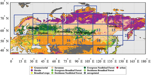
The current study focuses on fire activity in the Pan-Eurasian Experiment (PEEX) domain, covering thousands of kilometres from North Eurasian to China (Figure 1). PEEX program (https://www.atm.helsinki.fi/peex/) is a multi-scale, multi-disciplinary research initiative focusing on understanding biosphere–ocean–cryosphere–climate–society interactions and feedback to advance our understanding of interlinked grand challenges in the Arctic–boreal context/Northern Eurasia/Silk Road Region (Kulmala et al., 2015; Lappalainen et al., 2014, 2016, 2022; Petäjä et al., 2021). PEEX has introduced a concept design for a modelling platform and ground-based in situ observation systems for detecting land-atmosphere and ocean–atmosphere interactions. However, significant gaps remain over the PEEX domain, where little or no ground-based observational information is available (e.g. Vasileva et al., 2017). The gap can be partly filled by satellite remote sensing, which offers (to some degree) relevant parameters regarding atmospheric composition and land and water surface properties.

Figure 1. PEEX domain, selected areas, and selected locations. Background – land types map (https://lpdaac.usgs.gov/products/mcd12c1v006/, last access 25.08.2023). Coordinates of the selected areas are provided in the supplement (Table S2).

Aerosols emitted by forest fires are a special case in the PEEX domain since the strength of this source type depends on both climate change and human behaviour and since particles emitted by these fires have potentially significant radiative effects over the domain (PEEX science plan). In the current work, we examine monthly meteorological parameters (MP, namely temperature, precipitation, and soil moisture) by utilising ERA5 (European Centre for Medium-Range Weather Forecasts atmospheric reanalysis) modelled data to study possible links between weather/climate and fire activity for the summer months, May to August, for 2002–2022, in the PEEX domain. We study the spatial and temporal distribution of the fire activity indicators (FC and FRP) and aerosol/gas emissions (AGE), including AOD, CO, HCHO, and NO₂, to reveal how fire activity influences atmospheric composition. For a better understanding of the spatial features (e.g. response from the different vegetation zones, areas with different anthropogenic activity), selected cities, larger areas, and different latitudinal zones are considered. We introduce background values for selected variables (AOD, CO, HCHO, and NO₂) and analyse anomalies that exceed the background values. We calculate trends (over summers 2002–2022) for MP, fire indicators, and AGE over the PEEX domain and selected regions. For different land types, we estimate AOD:CO, AOD:HCHO, and AOD:NO₂ enhancement ratios (ER) and inter-compare satellite-derived ER with modelled (Akagi et al., 2011) and those utilized in SILAM (System for Integrated Modeling of Atmospheric Composition, Sofiev et al., 2009) model. For fire products that cannot be measured directly from satellites like BC, we utilise ground-based data from the AErosol RObotic NETwork (AERONET, Giles et al., 2019). This allows studying the temporal evolution of BC over selected cities over the PEEX domain where AERONET data are available. Our versatile approach, including analysis of the modelled climate data, atmospheric products retrieved from different satellite instruments, and ground-based products, reveals a complex picture of fire activity, its precursors, and consequences for the atmosphere.

The paper is structured as follows. In Sect. 2, we specify the PEEX domain. In Sect. 3, we introduce modelled, satellite and ground-based products utilised in the current study. Methods applied in the analysis are listed in Sect. 4. Fire activity in the PEEX domain (results from the modelled and satellite data analysis, including trends) is discussed in Sect. 5. Satellite-derived enhancement ratios over fire events are introduced in Sect. 6. Results from the analysis of the ground-based data are shown and discussed in Sect. 7. Conclusions are summarised in Sect. 8.

2. PEEX domain

PEEX domain (Figure 1) covers a wide range of land types and uses, environment conditions, population density, and thus air quality (PEEX science plan).

The northern part of the PEEX domain is in the Arctic zone. A defining feature of the arctic tundra, explained by permafrost and low precipitation, is the distinct lack of trees. Landscape diversity in arctic regions is poor due to the young age of surfaces, climate extremes, and, correspondingly, poor biota scope. The vegetation cover is noted for absolute domination of spore plants, algae, lichens, liverworts, and mosses. This biome has a short growing season. The Subarctic tundra has patchy, low-to-ground vegetation consisting of small shrubs, grasses, mosses, sedges, and lichens (Huemmrich et al., 2013).

The region south of the Arctic zones is occupied by boreal coniferous forests (dark-coniferous taiga). The boreal forest is the largest continuous land ecosystem in the world, covering about 14% of the Earth’s vegetated surface. It forms a “green belt” roughly between 45°N and 70°N. This biome is common in Scandinavia, European Russia, and Siberia. Its monotonous vegetation layer consists of 2–3 tree species: spruce, fir, cedar, pine tree, or larch (Grebner et al., 2013). In the direction to the South, forest dominants are oak, maple, linden, and ash tree species. Pine trees are spread over the driest sections with sandy and stony soils throughout the forest-steppe and steppe geographic range.

Boreal forest fires, in particular, Siberian, are known to be a major extra-tropical source of CO, as well as a significant source of BC (Lavoué et al., 2000) and other climate-relevant species to the atmosphere, dominating biomass burning sources at high latitudes (Paris et al., 2009).

Fires in the boreal forest region are widespread and extensive and produce a lot of smoke (Reisen et al., 2015). Boreal areas have been burning regularly for thousands of years and are often adapted to fires between May and October. In boreal ecosystems, future increases in air temperature may lengthen the fire season and increase the probability of fires, leading some to hypothesise positive feedback between warming, fire activity, carbon loss, and future climate change (Innes et al., 2000). Boreal fires burn into carbon-rich organic soils, releasing large quantities of trace gases and aerosols that influence atmospheric composition and climate. In the boreal forest, after CO2, CO, and CH4, the largest emission factors for individual gaseous species were HCHO, followed by methanol and NO₂ (Simpson et al., 2011).

Over the PEEX domain, we chose three latitudinal zones (the Northern Zone (NZ, 65ºN–73ºN), the Middle Zone (MZ, 55ºN–65ºN), the Southern Zone (SZ, 45ºN–55ºN) and 23 geographical areas (Figure 1, Table S2 in the supplement) characterized by different biodiversity, population density, and economic activity to study the influence of fire activity on atmospheric composition. Area 1 covers Scandinavia. Areas 2 to 20 are of 10º latitude by 20º longitude size. Areas 2–7 (numbering goes from west to east), 8–13, and 14–20 (except 19) cover three latitudinal zones from the north to south. Area 19 is central China (with Beijing in the centre). Areas 21–23 cover Kamchatka, the Russian Far East, and Taimyr (the most northern area). Analysis has been performed for all areas, while some results will be shown and discussed only for the selected areas (1-Scandinavia, 11-central Siberia, 19-central China).

Scandinavia (Area 1), with predominant pine and evergreen needleleaf forest, can be, in general (excluding the long-range pollution, e.g. dust, or forest fire emissions), considered a clean background area. With low population density and strict emissions policies, Finland has been rated among the world’s leading countries in many international comparisons of environmental protection standards, such as the Global Economic Forum’s regularly compiled Environmental Sustainability Index. The Finnish Forest Centre (https://www.metsakeskus.fi/en, last access 25.08.2023) maintains a network of multiple actors sharing knowledge, data, and maps to enable effective responses to forest fires.

Central Siberia (Area 11) is covered mainly by the deciduous needleleaf, mixed forest, and savannas. The population is concentrated mainly in a few industrial cities (e.g. Tomsk and Krasnoyarsk). Many wildfires are burning in eastern Siberia, creating massive smoke (Ponomarev et al., 2016). Wildfire is a critical environmental disturbance affecting forest dynamics, succession, and the carbon cycle in Siberian forests.

Mixed forest, grassland, and cropland are the main vegetation types in central China (Area 19). Note that in Areas 18 and 20, the results may be influenced by the transport of anthropogenic emissions from central China (e.g. Oh et al., 2015; Song et al., 2023).

Since the PEEX domain covers a wide range of land types and uses, environment conditions, population density, and thus air quality, the results obtained for different regions of the PEEX domain can be applied to similar regions around the globe.

3. Data

3.1. Satellite data

3.1.1. Fire count, fire radiative power, and aerosol optical depth from MODIS

Daily FC, FRP, and monthly mean AOD products are obtained from the Moderate Resolution Imaging Spectroradiometer (MODIS) satellites. The MODIS sensors (Salomonson et al., 1989) aboard NASA’s Terra and Aqua satellites (launched in December 1999 and May 2002, respectively) has been flying in a near-polar Sun-synchronous circular orbit for more than 20 years, observing the Earth–atmosphere system. MODIS/Terra crosses the Equator at 10:30 local time (descending node), and MODIS/Aqua crosses the Equator at 13:30 (ascending node). Both instruments have a viewing swath of 2330 km (cross-track) and provide near-global coverage daily.

The MODIS Terra Thermal Anomalies and Fire Daily (MOD14A1) Version 6 data are generated every 8 days at 1º×1º spatial resolution (user guide: http://modis-fire.umd.edu/files/MODIS_C6_Fire_User_Guide_B.pdf, last access 25.08.2003). The Science Dataset layers include the fire mask, pixel quality indicators, maximum FRP, and the position of the fire pixel within the scan (Justice et al., 2002). The fire mask is the principal component of the Level 2 MODIS fire product. Detailed information on climate modelling grid for the fire products and their estimation methodology can be found in, e.g., Kaufman (2002) and Giglio et al. (2016).

Cloud screening quality in the fire detection algorithm is critical. Dense cloud cover during the burning season may hinder the detection of small fires, and, hence, the observed FC may be smaller than the actual FC. Due to the fire being obscured by clouds and smoke or not burning actively during the satellite overpass, about one-third of all fires in Siberia had no active fire points detected (de Groot et al., 2013). Information about the background brightness temperature, required for FRP calculations (e.g. Giglio et al. (2003)), is sometimes unavailable in neighbourhoods of thick cloud cover and extensive fires. Thus, the mean FRP calculations do not include fire pixels in the abovementioned cases and those detected at scan angles above 40°.

Apart from dense cloud cover, other limitations to the fire detection process from the MODIS observations also exist (Giglio et al., 2003, 2016). Many small agricultural fires are missed in the detection process because they are too small to raise the brightness temperature of the pixel. Satellite wildfire detection also suffers from false detections caused by anthropogenic heat sources such as gas flares and some large industrial facilities (Giglio et al., 2016).

The Terra MODIS active fire product has primarily been validated using coincident, high-resolution fire masks derived from Advanced Spaceborne Thermal Emission and Reflection Radiometer (ASTER) imagery. The MOD14 Collection 6 daytime global commission error was 1.2% (Giglio et al., 2016).

Measurements of MODIS FRP have an uncertainty of 26.6% at the one sigma level; the fire location drives uncertainties in MODIS FRP within the point spread function and does not depend on scan angle (for more details, see Freeborn et al., 2011, 2014). The FRP dependence on the view zenith angle has been reported by Li et al. (2018).

Cumulative over-month FRP and FC have been calculated and utilised in the analysis. Fires classified as 8 or 9 (nominal or high quality, respectively) have been considered (Justice et al., 2002). Because FC and FRP vary across a wide range of values and are distributed in a non-linear pattern (Figure 2), some analyses were conducted at logarithmic (lnFC and lnFRP) scales.

Figure 2. Cumulative FRP (MW, 10⁶) over the summer season (May to August) over the PEEX domain for 2002–2022 obtained from the MODIS instrument.

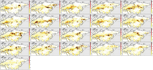
As shown later in the analysis, FRP footprints closely follow the fire distributions or fire counts; the spatial correlation between FC and FRP is relatively high (0.7–0.9). Thus, when discussing the spatial distribution of fires, we show results for the FRP only. When calculating statistics, both FC and FRP are considered.

In this paper, MODIS/Terra AOD at 550 nm from the C6.1 Dark Target Deep Blue merged monthly product (MOD08_M3, 2002–2022, https://ladsweb.modaps.eosdis.nasa.gov/, last access 25.08.2023), referred hereunder as AOD, are used. Monthly AOD product shows a good performance globally with a slight positive bias, though regional differences in the performance exist (e.g. Sogacheva et al., 2018, 2020; Wei et al., 2019).

3.1.2. CO (MOPITT)

Measurement of Pollution in the Troposphere (MOPITT, 2018, https://terra.nasa.gov/about/terra-instruments/mopitt, last access 25.08.2023; Deeter et al., 2022) on board Terra is a nadir viewing infrared radiometer with a specific focus on the monitoring of distribution, transport, sources, and sinks of carbon monoxide in the troposphere. MOPITT is one of the earliest satellite sensors to use gas correlation spectroscopy to obtain information on CO profiles. MOPITT measurements yield atmospheric profiles of CO volume mixing ratio and CO total column values using near-infrared radiation at 2.3 µm and thermal-infrared radiation at 4.7 µm (Edwards et al., 2004; Liu et al., 2011). MOPITT’s spatial resolution is 22 km at nadir, and it “sees” the Earth in swaths that are 640 km wide.

In this work, MOPITT CO gridded monthly means (MOPITT user guide) have been utilized (https://eosweb.larc.nasa.gov/project/mopitt/mop03jm_v008, last access 20.08.2023). V8 products have been validated; a summary of validation results can be found at https://www.acom.ucar.edu/mopitt/validation/val-retr.shtml (last access 20.08.2023).

3.1.3. HCHO and NO₂ (OMI)

Tropospheric NO₂ and HCHO products utilised in the current study are obtained from the Ozone Monitoring Instrument (OMI), launched in July 2004 onboard the National Aeronautics and Space Administration (NASA) Aura satellite (Levelt et al., 2006). It is an imaging spectrometer covering the wavelength range from 270 to 500 nm to monitor, e.g. ozone, NO₂, and other trace gas column densities with a spatial resolution of about 13 × 24 km² (at nadir). OMI is operated on a sun-synchronous orbit, with an overpass time of about 13:45 local time, and it reaches global coverage in one day. Since early 2008, OMI has suffered from a so-called “row anomaly” and lost several cross-track position data (Boersma et al., 2007, 2008, 2011). The row anomaly affects data quality (e.g. He et al., 2020). Therefore, pixels with row anomaly are excluded, which reduces the amount of data available from the instrument despite global coverage.

In this study, monthly mean tropospheric column densities of NO₂ and HCHO from the EU Seventh Framework Programme (FP7) Quality Assurance for Essential Climate Variables (QA4ECV) project for the years 2005–2020 were used. This project aimed to provide a consistent long-term time series and fully traceable quality assurance for the global satellite NO₂ and HCHO column densities, including the OMI instrument (e.g. Zara et al., 2018). The QA4ECV data are available as Level 3 daily and monthly data via the TEMIS website (http://www.temis.nl/qa4ecv/no2.html and https://www.temis.nl/qa4ecv/hcho/hcho_month.php). The validation study by Compernolle et al. (2020) shows that the QA4ECV OMI NO₂ vertical column densities tend to be negatively biased (from −1 × 10¹⁵ to −4 × 10¹⁵ molec/cm²) to ground-based MAX-DOAS observations. Also, for QA4ECV HCHO product, a negative bias of about −25% is found at high HCHO concentrations (de Smedt et al., 2021), which can partly be explained by low OMI spatial resolution (Kramer et al., 2008).

As the QA4ECV data are available only until the end of 2020, Level 3 NO₂ and HCHO Tropospheric column observations from OMI for the two latter years included in this study were obtained from NASA OMNO2d V3 (Krotkov et al., 2017) and OMHCHOd (González Abad et al., 2015; Sun et al., 2018) data products. Level 3 monthly means of these observations were obtained via the NASA Giovanni tool (https://gpm.nasa.gov/data/sources/giovanni, last access 25.08.2023). Krotkov et al. (2017) show that in an urban environment, NASA version 3 NO₂ tends to have a systematically negative bias compared to ground-based measurements. A validation study by Zhu et al. (2020) showed that the NASA OMI HCHO tend to be also negatively biased (<20%) at high HCHO concentrations but positively biased (>60%) at low concentrations. A detailed comparison of the QA4ECV and NASA fitting approaches showed small (<4%) differences between NO₂ QA4ECV and OMNO2d V3 (Compernolle et al., 2020; Zara et al., 2018).

3.2. Ground-based data – AERONET

AERONET is a ground-based, internationally federated, globally distributed network of well-calibrated sun photometers (Holben et al., 1998). It has provided measurements of aerosol optical, microphysical, and radiative properties in high temporal resolution for over two decades. AERONET locations, primarily continental, are not representative of the global mean, but they can be used for characterising local and areal aerosol conditions and properties. AERONET aerosol optical depth (AOD) is derived from direct beam solar measurements from ultraviolet to infrared.

Ground-based sun photometers provide accurate measurements of AOD (uncertainty ~0.01–0.02, e.g. Eck et al., 1999; Sinyuk et al., 2020) because they directly observe the attenuation of solar radiation without interference from land surface reflections in the spectral range 340–1640 nm.

Spectral AOD can be obtained from AERONET direct sun measurements. AERONET inversion product offers other aerosol optical properties, such as single scattering albedo (SSA), refractive indices, and the column-integrated aerosol size distributions at the sky radiance wavelengths (Holben et al., 1998). Imaginary indices and volume size distributions can be further applied to estimate the concentration of absorbing components (e.g. Arola et al., 2011; Schuster et al., 2016). In our study, we estimated the concentrations of absorbing organic and black carbon concentrations at selected AERONET sites.

3.3. Modelled data from ERA5

ERA5 is the fifth generation European Centre for Medium-range Weather Forecast (ECMWF) atmospheric global climate reanalysis. It provides a consistent view of the water and energy cycles at the surface level over several decades. In this work, we use monthly averaged skin temperature (temperature of the surface of the Earth, called here down temperature), soil moisture (volume of water in soil layer 1 (0–7 cm)), and monthly cumulative precipitation (total precipitation) aggregated to 1º×1º spatial resolution. ERA5 products can be downloaded from the Copernicus Climate Data Store (https://cds.climate.copernicus.eu/#!/home, last access 21.08.2023).

4. Methods

4.1. Temporal and spatial resolution

Let $\mathit{X}\left(\mathit{i},\mathit{m},\mathit{n}\right)$ be a variable in Area i, for month m in year n. The spatial index, i, goes through all nominal resolution (1º×1º) grid cells (or larger areas). The month index, m, varies from 1 to 4, covering the four calendar months (May, June, July, and August) in the fire season. The time index, n, varies from 1 to 21, covering years 2002–2022. In the following analysis, each calendar month is treated separately (to remove different seasonal effects on different variables). Each subset of data covers a period of 21 years (for a single calendar month). The variables are FRP (or lnFRP), FC, AOD, HCHO, CO, NO₂, temperature, precipitation, and soil moisture.

4.2. Absolute and relative anomalies

Anomaly for a variable $\mathit{X}\left(\mathit{i},\mathit{m},\mathit{n}\right)$ is obtained by subtracting the corresponding median value:

(1) $\mathit{Xanom}\left(\mathit{i},\mathit{m},\mathit{n}\right)=\mathit{\hspace{0.17em}}\mathit{X}\left(\mathit{i},\mathit{m},\mathit{n}\right)-\tilde{X}\left(\mathrm{i},\mathrm{m}\right)$(1)

where the median $\tilde{X}\left(\mathrm{i},\mathrm{m}\right)$ (Figure S1, Supplement) is obtained from the subset of years from the period 2005–2017 for the considered pixel $\mathit{i}$.

The anomaly values are used to highlight better the connections between different variables with different ranges of actual values.

The relative anomaly $\mathit{Xrel}\left(\mathit{i},\mathit{m},\mathit{n}\right)$ is obtained by scaling the anomalies by the median values:

(2) $\mathit{Xrel}\left(\mathit{i},\mathit{m},\mathit{n}\right)=\frac{\mathit{X}\left(\mathit{i},\mathit{m},\mathit{n}\right)-\tilde{X}\left(\mathrm{i},\mathrm{m}\right)}{\tilde{X}\left(\mathrm{i},\mathrm{m}\right)}$(2)

The relative anomaly makes comparing different variables with varying ranges of variance easier.

4.3. Background AOD, HCHO, CO, and NO₂

The background (BG) value $X_{\mathit{BG}}\left(\mathit{i},\mathit{m}\right)$ for each pixel, i, and each calendar month m is taken as the minimum value over the years:

(3) $X_{\mathit{BG}}\left(\mathit{i},\mathit{m}\right)=\mathit{mi}{n}_{\mathit{n}=1\dots 21}\mathit{X}\left(\mathit{i},\mathit{m},\mathit{n}\right)$(3)

The background value can be considered a proxy for the anthropogenic and natural emissions that are unrelated to wildfires. A local value is used since we assume that the background signal, e.g. anthropogenic activities, is spatially highly variant. It can be further assumed that removing local background from the signal would make the wildfire response better comparable between different areas and make conclusions on a larger scale possible.

4.4. Scaled anomalies

Instead of using the median values to scale the data, we tested another method. First, the background value $X_{\mathit{BG}}\left(\mathit{i},\mathit{m}\right)$ is subtracted from the variable. The background (minimum) value can better represent the background independent of wildfires. In contrast, the median values used for the anomaly data $\mathit{Xanom}\left(\mathit{i},\mathit{m},\mathit{n}\right)\mathit{\hspace{0.17em}}$ may contain the contribution of fires, although averaged over the years. These anomalies are scaled from 0 to 1 to allow better comparison between variables of different absolute scales. The scaling is done by dividing with the local maximum value over the years for the month considered:

(4) $X_{\mathit{max}}\left(\mathit{i},\mathit{m}\right)=\mathit{ma}{x}_{\mathit{n}=1\dots 21}\mathit{X}\left(\mathit{i},\mathit{m},\mathit{n}\right)$(4)

The scaled anomaly $X_{\mathit{SA}}\left(\mathit{i},\mathit{m}\right)$ for variable X is defined as

(5) $X_{\mathit{SA}}\left(\mathit{i},\mathit{m}\right)\mathit{\hspace{0.17em}}=\frac{\mathit{X}\left(\mathit{i},\mathit{m},\mathit{n}\right)-{\mathit{X}}_{\mathit{BG}}\left(\mathit{i},\mathit{m}\right)}{X_{\mathit{max}}\left(\mathit{i},\mathit{m}\right)}$(5)

4.5. Trend analysis

Decadal trends of the FC, FRP, AOD, atmospheric gases (CO, HCHO, NO₂) and meteorological parameters (T, P, SM) were calculated using the Climate Data Toolbox for Matlab (https://chadagreene.com/CDT/CDT_Getting_Started.html, Greene et al., 2019).

4.6. Aggregation

For the 23 areas (subsets of the PEEX domain, Figure 1), three latitudinal zones (NZ, MZ, and SZ; for details, see Sect. 2), and the whole PEEX domain, the original values were first aggregated over the area and then processed as described above (e.g. for the anomalies and scaled values). The result would differ if the nominal resolution (1º×1º) values were first processed and then aggregated into the area.

5. Results

5.1. Fire activity in the PEEX domain over the last two decades

Cumulative lnFRP over the summer season (May–August) for the PEEX domain for years 2002–2022 is shown in Figure 2. Although some hotspots of fires can be recognised almost every year (e.g. Siberia, Eastern Europe), the location and energy release from fires change from year to year and from month to month (Figure S2, Supplement).

The distribution of fire characteristics over the area is far from homogenous. The fire frequency is higher in the populated regions of the European part of Russia, Southern Siberia, and the south of the Russian Far East. The spatial extent of fires is significantly higher in less populated central Siberia and the northern Far East, where fire protection is also lower (https://efi.int/sites/default/files/files/publication-bank/2020/efi_wsctu_11_2020.pdf, last access 21.08.2023). Among climate domain subregions, boreal forests in Eurasia and North America have the largest absolute area of forest loss due to fire and, along with subtropical forests of Australia and Oceania, the highest percentage of forest loss due to fire from the total 2001–2019 forest loss area (Tyukavina et al., 2022).

It is important to note that while forest fires are generally considered a natural phenomenon in boreal forests, the fire ignitions in Russia are often human-induced (Frédéric et al., 2008). Jones et al. (2022) suggest that lightning plays a key role as a fire ignition source throughout the boreal forest zone. While the ignitions play an important role in the complex fire activity system, climate variables significantly affect the environmental conditions (e.g. drought) that define how severe fires will develop.

Some of the most extensive burning episodes in the PEEX domain have been widely investigated. During the 2003 fire season, blazes in the taiga forests of Eastern Siberia were part of a vast series of fires across Siberia and the Russian Far East, northeast China, and northern Mongolia. More than 200,000 km² were burned from 14 March to 8 August 2003, of which 71.4% was forest, 9.5% humid grassland, and 2.15% bogs or marshes. From 1996 to 2003, 32.2% of the forested area and 23.36% of the total area were burned, and 13.9% of the total area was affected by fires at least twice. Direct carbon emissions from these fire events in 2003 were around 400–640 Tg (Huang et al., 2009).

During the summer of 2010, central European Russia endured the driest and hottest July and August ever recorded. Witte et al. (2011) reported anomalously high temperatures (35º–41°C, compared to average temperatures of 15º–20°C usually observed in the summer season) and low relative humidity (9–25%) from mid-June to mid-August 2010. The intense heat and drought were favourable conditions for hundreds of wildfires within European Russia. They burned forests, grasslands, croplands, fields, and urbanised areas across a massive region around Moscow (Shvidenko et al., 2011), severely affecting the air quality (Elansky et al., 2011; Fokeeva et al., 2011; Golitsyn et al., 2012) and causing strong aerosol radiative effects (Chubarova et al., 2012). Based on the information retrieved from different environmental satellites, significant emissions of aerosols and trace gases such as CO, HCHO, NO₂, NH₃, and HCOOH have been reported (Huijnen et al., 2012; R’Honi et al., 2013; Yurganov et al., 2011). These smoke plumes drifted a thousand kilometers away to Finland (Mielonen et al., 2012) and Ukraine (Zvyaginstev et al., 2011).

In 2012, 2013, 2015, and 2017, most fires burned through taiga in the remote parts of eastern and central Siberia. Since the area has a low population density, less interest in those fires has been shown in both media and scientific publications. However, the burnt regions cover thousands of square kilometres, and emissions to the atmosphere have been enormous. In 2019, the total extent of burned-out areas and the emissions of harmful gases and fine aerosols in Siberia were abnormally high. Wildfires affected an area of 72.4 thousand km² in Siberia, which constituted 42% of the area of wildfires that occurred this year throughout Russia (Voronova et al., 2020).

Bondur et al. (2023) reported that overall, the burnt regions in Russia decreased from 2001 to 2022, while the average annual values of FRP increased, indicating that during the 20 years’ fires have become more intense. The largest areas of wildfires in Russia within a month were in the Siberian Federal District in May 2003, in the European part of Russia and the Ural Federal District in April 2009, in central European Russia in July–August 2019, and in the Far Eastern Federal District in July and August 2021.

Within the summer season, the temporal occurrence of fires has spatial dependence (Figures S2 and S3, Supplement). Eastern Europe, where fires are mainly due to the reckless burning of agricultural residues that often spread and become large-scale forest fires, is burning more often in May (e.g. Leino et al., 2014; Markowicz et al., 2016; Stohl et al., 2007). Early to mid-summer is the primary season for fires in the far North (above 65ºN), but the active fire season in middle latitudes can have a second peak in August and occasionally in September after agricultural harvests in the fall (Voronova et al., 2020). A typical fire season in Russia starts in the south around March after the snow melts in the spring (indicating field preparation) and gradually moves to the north as the weather warms and the snow melts (Romanenkov et al., 2014). The earliest fires are in steppe regions along the Chinese-Mongolian border. Many of these are relatively short-lived agricultural fires; others may be extensive. Thus, following the intra-summer fire frequency variation, the analysis was performed in monthly resolution.

5.2. Background monthly values for aerosol/gas emissions

Having up to 21 years’ records of satellite data (2002–2022 AOD and CO, 2005–2020 for HCHO and 2005–2022 for NO₂), which includes periods of different anthropogenic activity (e.g. de Leeuw et al., 2022; Sogacheva et al., 2018) and natural variations (e.g. biomass burning, dust transport, e.g. Proestakis et al., 2018), we created background database for AOD, CO, HCHO, and NO₂ over the PEEX domain. The background signal presumably has high spatial variation and some seasonal variation; thus, the months of May to August are treated separately. Wildfire signals could be considered of sporadic nature and might then show up more clearly in the data.

Utilising the 1º×1º monthly resolution products, we extracted the monthly minimum (for the whole satellite parameter measurement period) and combined them into the product, which we called a background (BG, see Sect. 4.3 for details). We could not decompose the background into the natural and anthropogenic components with the tools available for this research. Nevertheless, this product can reveal a temporal variation from the minimum concentration measured at 1º×1º resolution over the last two decades. Using a local minimum for each grid cell, we attempt to remove the effect of the local background and stationary emissions, including both anthropogenic and natural sources, which have high spatial variation and possibly seasonal variation but some interannual temporal consistency. Removal of the BG allows us to focus on the effects of wildfire emissions, presumably more sporadic, on a larger spatial scale.

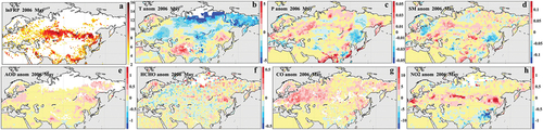
BG monthly values for AOD, HCHO, CO, and NO₂ for May to August are shown in Figure 3. For regions where the anthropogenic activity remained nearly constant during 2002–2022 (which is not valid for, e.g., China (e.g. de Leeuw et al., 2022; Sogacheva et al., 2018)), variations in the variables between the months can be assigned to the natural variations.

Figure 3. For AOD, HCHO, CO, and NO₂ (panels left-right), background monthly values (May to August, panels top-down) obtained from 2002–2022 (for AOD and CO; 2005–2020 for HCHO; 2005–2022 for NO₂) monthly products.

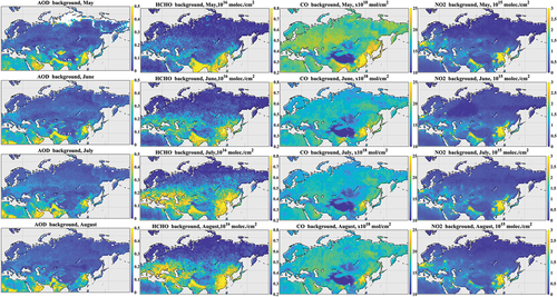
AOD BG over Russia in May is about 0.1, with some increase towards July and a subsequent decrease in August. A similar temporal tendency is observed for HCHO, which also shows a gradual latitudinal increase towards July in the direction to the north. CO shows clear maxima in the background in May and a second maxima in August. In June and July, CO is lower. NO₂ shows intense anthropogenic activity in China and central Russia, with a high AOD, HCHO, and CO background.

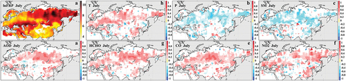
An example of how removal of the pixel-level monthly background values (as defined by eq.3 and shown in Figure 3) changes the spatial distribution of the monthly variables is presented in Figure 4. The actual mean values for T, P, SM, AOD, HCHO, CO, and NO₂ are shown in the upper panel, whereas the lower panel shows the spatial distributions after the background value has been removed from the monthly mean data. Note that the FRP background is 0.

Figure 4. For July 2002–2022, mean actual values (upper panel) for lnFRP (a), T (b), P (c), SM (d), AOD (e), HCHO (f), CO (g), and NO₂ (h) and mean monthly values (lower panel) for the same variables after removal of the background values (except for lnFRP, which remains unchanged).

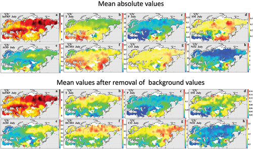
The temperature deviation from the background steadily increases towards the north and reaches its highest values in the north of central Russia and the Russian Far East. A similar tendency is shown by soil moisture. Variation in precipitation anomaly (deviation from the background) in the boreal area is moderate compared with southeast Russia and China.

AOD is deviating more (0.4–0.5) from the background over Siberia, which is characterised by the highest fire activity in the PEEX domain. A footprint from the high lnFRP over cropland/grasslands is not recognised in the distribution of the AOD. This confirms our previous conclusion about the low response of the AOD to the cropland fires. Other than Siberian, a high deviation of the AOD from the background values is in China, where anthropogenic particles contribute strongly to the AOD. CO shows a spatial distribution similar to AOD.

HCHO shows behaviour similar to temperature (latitudinal increase in the direction to the north). However, forest fires in central Siberia can be recognised in the highest (above 3.5 × 10¹⁵ molec/cm²) HCHO anomalies. As with actual monthly mean values, regions with a high level of anthropogenic pollution can be recognised in the spatial distribution of NO₂ anomalies after removing the BG values. The response of the NO₂ on forest fires is not so clear and considerably lower than the industry’s contribution to the total NO₂ concentration.

5.3. Spatial and temporal correlation between FRP, meteorological parameters, and atmospheric composition

5.3.1. PEEX domain

The correlation coefficients (R) between the lnFRP and T, P, SM, AOD, HCHO, CO, and NO₂ have been calculated from monthly mean data for each 1°× 1° grid (using 3°× 3° moving window) for 2002–2022 (2005–2022 and 2005–2020 for NO₂ and HCHO, respectively). The spatial distribution of the correlation coefficients for the actual values for July is shown in Figure 5.

Figure 5. Mean lnFRP for July 2002–2022. (a) Spatial distribution of the correlation coefficients (p-value < 0.05) between lnFRP and temperature, T (b), precipitation, P (c), soil moisture, SM (d), AOD (e), HCHO (f), CO (g), and NO₂ (h) for July 2002–2022.

Over the PEEX domain, lnFRP shows a negative correlation to precipitation (P) and soil moisture (SM) (R is −0.28 and −0.30, respectively). The correlation between lnFRP and temperature (T) is positive (0.28) reaching values of 0.4–0.8 over the areas with high FRP. As expected, higher temperatures, lower precipitation, and soil moisture are favourable for a more intensive fire activity. Also, AOD, CO, HCHO, and NO₂ show positive responses to the increased fire activity (0.27, 0.29, 0.33, and 0.29 respectively) (Table 1).

Table 1. For July, for the whole PEEX domain and different land types, the mean statistically significant (p < 0.05) correlation coefficients between lnFRP and T, P, SM, AOD, CO, HCHO, and NO₂.

	T	P	SM	AOD	CO	HCHO	NO2
PEEX domain	0.28	−0.28	−0.30	0.27	0.29	0.33	0.29
Land type
grass	0.27	−0.25	−0.25	0.12	0.25	0.27	0.25
shrubs	0.38	−0.32	−0.36	0.28	0.21	0.30	0.35
broadleaf crops	0.29	−0.26	−0.25	0.20	0.21	0.25	0.38
forest	0.24	−0.29	−0.33	0.32	0.34	0.34	0.22
savannas	0.27	−0.28	−0.31	0.32	0.30	0.36	0.33

AOD, CO, and HCHO responses on the lnFRP are stronger for forest and savannas (tundra). NO₂ response on the lnFRP is stronger for shrubs, broadleaf crops, and savannas. Removal of the background (BG) increases the correlation of the lnFRP with AOD (from 0.12 to 0.21) for grass and with NO₂ (from 0.22 to 0.28) for forest (Table 1).

5.3.2. Case studies over latitudinal zones

As discussed above, the seasonality of wildfires within the PEEX domain depends on the location (Figures S2, S3). The study area can be roughly divided into three major latitudinal vegetation types: croplands in the southern part of the study area, Siberian boreal forest in the middle, and open shrubland and savannas in the northern part (approx. SZ, MZ, and NZ, respectively, as defined in Sect. 2). Fires in the cropland regions are typically agricultural and occur most frequently in May before the growing season starts, and in August–September, at the end of the growing season (post-harvesting). In contrast, fires in the Siberian boreal forest region occur most frequently in July and August. The fire occurrence in the northern part is notably lower than in the two other regions. Since open biomass burning varies widely in terms of ignition processes, size, intensity, spread rate, duration, seasonality, frequency of recurrence, and emission characteristics depending on ecosystem type, location, prevailing weather, and fuel characteristics (Ichoku et al., 2012; Wan et al., 2023), the results for different land types are discussed separately.

As an example of cropland fires, we consider May 2006, when intensive fires in southern Russia and Kazakhstan occurred. Figure 6 shows a monthly spatial distribution of the lnFRP and anomalies of meteorological parameters (temperature, precipitation, and soil moisture), AOD, and trace gases (CO, HCHO, and NO₂). Over the region, meteorological conditions over burning areas were close to the median over the study period; no apparent anomalies in the AOD, HCHO, and CO were observed, while the NO₂ anomaly was positive. Cropland fires have also been observed in August 2013. For those fires, the conclusions made for the dependence of the lnFRP from the meteorological parameters, AOD, and trace gases are similar to those from May 2006 (Figure 6).

Figure 6. For May 2006 (intense cropland fires in southern Russia and Kazakhstan), satellite lnFRP and ERA5 anomalies of meteorological parameters (T, P, and SM), satellite AOD and gas emission (HCHO, CO, NO₂) calculated with respect to median (2005–2017) values.

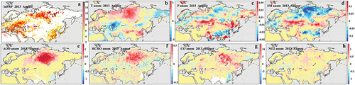
For the Siberian boreal forest region (MZ), results indicate that anomalies in the meteorological parameters appeared to be more critical to the occurrence of the fires than for the cropland fires (Figure 7). August 2013 was chosen for a more detailed investigation as it is one of the most intense fire months of the study period in the Siberian boreal forest. The results show a clear positive temperature anomaly (up to 5°C) and a negative soil moisture anomaly (below −0.1 m³/m³) for this region. The precipitation anomaly was slightly negative (up to 0.05 m). AOD, HCHO, and CO positive anomalies (>1, up to 0.5 and above 10, respectively) mimic the footprint of the burnt region, while the NO₂ anomaly was minor (around 0.1).

Figure 7. For August 2013 (intense fires in Siberia and eastern Europe), same as Figure 6.

For August 2013, we also show scatter plots (for actual values, as in Figure 8, and anomalies, as in Figure 9) between monthly cumulative lnFRP and meteorological parameters, aerosol and gas concentrations, with colour reflecting the latitude (vegetation zone).

Figure 8. For August 2013, scatter plots of lnFC versus lnFC(a), meteorological parameters (temperature, (b); precipitation, (c); soil moisture, (d)), AOD (e), HCHO (f), CO (g), and NO₂ (h) with colour showing the latitude dependence (colourbar, latitudinal zones). Red dots correspond to the Sakha (Russia) area; magenta dots correspond to Jinan (China) area.

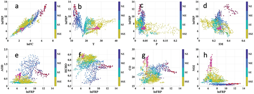
Figure 9. As Figure 8, scatter plot for anomalies.

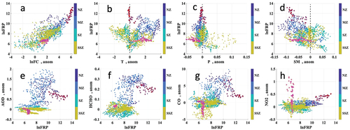
The response of meteorological variables, as well as trace gas and aerosol concentrations on fire radiative power follows closely the distribution of the vegetation types (SZ, cropland; MZ, forest; NZ, tundra (see Sect. 4.1), and SSZ – grassland zone south of SZ, outside the PEEX domain). The maximum value of the monthly accumulated 1º×1º grid lnFRP remained below 8 in the SSZ, while in the SZ, MZ, and NZ, the lnFRP was as high as 10, 13, and 11, respectively. Thus, fires are most intensive in the MZ based on the energy release.

A clear linear relation exists between lnFC and lnFRP (Figure 8(a), Table 2). Correlation between lnFC and lnFRP is highest in the MZ (0.91, boreal forest) and decreases towards the South. lnFRP positively correlates with the lnFC anomalies (Figure 9(a)) in the MZ (R = 0.79). The correlation is lower in the NZ and SSZ, while in the SZ, the correlation between lnFC and lnFRP is negative.

Table 2. For August 2013, correlation coefficients between different variables (Var1, Var2, actual values, and anomalies) for four zones (NZ, MZ, SZ, and SSZ) defined in Sect. 2. Statistically not significant values are replaced with *.

	Zones	NZ	MZ	SZ	SSZ	NZ	MZ	SZ	SSZ
Var1	Var2	for actual values				for anomalies
lnFC	lnFRP	0.88	0.91	0.85	0.56	0.35	0.79	−0.41	0.10
T	lnFRP	*	−0.62	0.42	0.40	−0.24	0.70	−0.44	−0.43
P	lnFRP	0.17	0.15	−0.62	−0.59	0.18	−0.24	−0.13	−0.10
SM	lnFRP	*	−0.43	−0.59	−0.66	*	−0.65	*	*
lnFRP	AOD	0.22	0.68	*	−0.44	0.24	0.69	0.10	0.15
lnFRP	HCHO	0.39	0.53	0.25	−0.49	0.26	0.58	0.11	0.25
lnFRP	CO	0.45	*	0.48	−0.08	0.34	0.73	*	−0.16
lnFRP	NO2	*	−0.60	−0.30	−0.41	0.35	0.57	−0.37	−0.11

lnFRP shows a negative correlation with actual T in the MZ and positive correlation in the SZ and SSZ. Temperature anomalies show the opposite (in sign) to actual values correlation. LnFRP is more sensitive to P and SM in SZ and SSZ.

The difference between zones in the response of AOD and trace gases to the lnFRP is more evident. As shown earlier, the AOD background is considerably higher in the SSZ, which is more populated and where the industry is distributed more densely and evenly compared to the MZ. However, the actual AOD values for the forest burning events (MZ) were considerably higher than the AOD over the cropland fires (SSZ) (Figure 8(e)). We can suggest several reasons for this difference. First, cropland fires are often less intensive; thus, fewer aerosol particles are emitted into the atmosphere (e.g. Hall et al., 2024). Second, particles emitted from cropland fires are smaller and can be below the detection limit for satellite retrieval (e.g. Reid et al., 2005). Third, smouldering from forest fires is often more intensive and lengthier (e.g. Rein & Huang, 2021). AOD response to lnFRP is positive in the MZ (R = 0.68) and negative (R = −0.44) in the SSZ. This implies that the AOD values in the SSZ are unrelated to wildfires.

Two “clouds” of points, marked with red and magenta circles in Figures 8 and 9, often show behaviour that is unexpected for their latitudinal zones. A set of red dots has been allocated to Sakha (63º–68º N, 110º–120º E), Russia. lnFRP was very high in this region, while temperature and precipitation anomalies were close to 0. AOD, HCHO, and CO anomalies were decreasing with increasing lnFRP. NO₂ anomaly was exceptionally high, which may indicate sporadic intensive anthropogenic activity (mining, forestry) in this region. A set of magenta dots is allocated to Jinan (34º–40º N, 112º–122º E), China. In this region, CO and NO₂ values were exceptionally high, deviating much from the similar lnFRP values (of ca. 6.5). Deviation of anomalies was also high (from 0.5 to −4.5 and from −0.2 to 1.2 for CO and NO₂, respectively). Because of the different relation to lnFRP, those points were excluded from the statistical analysis performed in this section. One of the reasons for the exceptional behaviour can be the fact that MODIS fire detection false alarms are possible (https://modis-fire.umd.edu/files/MODIS_C6_Fire_User_Guide_C.pdf). The other possible reason is chemical transformations of the emitted gases and mixing with other particles of both anthropogenic and natural origin (e.g. Péré et al., 2009).

Similar (as in Figure 6) anomaly patterns for cropland fires (in, e.g., May and August 2008, Figure S4, supplement) and for forest fires (as in Figure 7 in, e.g., August 2017 and July 2019, Figure S5, supplement) can be recognised. This allows us to draw general conclusions on the difference between cropland/grassland and forest fires on the FRP response on MP anomalies and AGE response on the lnFRP. Temperature, precipitation, and soil moisture are more critical for the occurrence of forest fires, while other factors than meteorological factors (e.g. anthropogenic activity, post-harvest burning) often cause cropland fires (e.g. Hall et al., 2021; Jung & Kang, 2021). Cropland fires are not the main reason for positive AOD, HCHO, and CO anomalies in more populated and economically active zones. This supports the hypothesis that anthropogenic emissions contribute most to the AOD, HCHO, and CO concentration measures from satellites in those areas. AOD, HCHO, and CO anomalies closely follow biomass burning in relatively clean areas. The fire signal in NO₂ concentration is also low compared to the anthropogenic emissions, though this signal from fires is more pronounced in the South compared to the much less populated North.

The differences between cropland/grassland fires and forest fires in the lnFRP response on MP anomalies and AGE response on lnFRP shown for selected cases (Figures 6–9) are confirmed by the latitudinal analysis applied to available data. Since the general distribution of the vegetation zones in the PEEX domain is close to latitudinal (Figure 1), we, using the same approach as in Sect. 5.3 (applied there to the whole PEEX domain), calculated the correlation coefficients between variables for three latitudinal zones, defined in Sect. 4.4: SZ, MZ, and NZ (predominantly cropland and forest, forest, and tundra, respectively).

The difference between zones in the lnFRP response on MP anomalies and AGE response on lnFRP is clear (Table 2). MZ shows the highest response of the lnFRP on the MP (R is 0.70, −0.24, −0.65, for T, P, and CM, respectively) and the highest AGE response on the lnFRP (R is 0.58, 0.73, 0.57 for HCHO, CO, and NO₂). In the MZ, AOD anomalies may be as high as two during the fire events, with a correlation of R = 0.58 with lnFRP.

5.3.3. Areal analysis

Local warming and vegetation change patterns are variable across the Arctic (Post & Mack, 2022) and Siberia. Having shown the difference between the latitudinal zones in the (i) FRP response on the meteorological conditions (temperature, precipitation, soil moisture) and (ii) response of the AOD and emitted gases (HCHO, CO, NO₂) on the FRP (Sect. 5.5), we look deeper into a longitude dependence between the logFRP and other variables for more homogeneous (as regarding vegetation cover and anthropogenic activity) areas and, by looking at the averaged over each area separately data, consider a possible long-range transport of the atmospheric constituents from the emission sources (in our study – burnt regions, e.g. Jaffe et al., 2004; Ngoc Trieu et al., 2023).

Twenty-three selected areas (Figure 1; Table S1, supplement, Sect. 2) were defined. The FRP and precipitation were accumulated, while temperature, soil moisture, AOD, HCHO, CO, and NO₂ were averaged over each selected area. Since the difference in seasonality (difference between the summer months, in our case) has been revealed in the fire activity between different latitudinal zones, results are shown monthly. Note that Area 1 is bigger; thus, cumulative FRP and cumulative precipitation in this area cannot be compared directly to the same variables in the other areas.

5.3.3.1. Matrix plots for actual values and scaled anomalies

For the 23 areas (Figure 1), the temporal distributions of the monthly variables are shown as matrix plots (Figure 10). Each row on the plot (along the x-axis) represents a time series for one area, denoted by a number on the y-axis. Top-down placement of the areas allows tracking possible variations from the North to the South. These matrix plots allow us to study the temporal evolution of burning periods (FRP, FC) following the behaviour of other variables (MP, AGE). At the same time, this kind of visualisation allows checking if an increase in, e.g. AOD and/or trace gases, is following burning activity or not (which shows the predominant origin of the pollutions: natural or anthropogenic).

Figure 10. Temporal and spatial distribution of FRP, temperature (T), precipitation (P), soil moisture (SM) (upper panel), and AOD, HCHO, CO, and NO₂ (lower panel) for July. The Y-axis shows the Areas (1–23) defined in Figure 1, while the X-axis shows the time (years). Vertical black dashed lines separate 5-year periods (e.g. 2006–2010 from 2011–2015), whereas horizontal green lines divide different latitudinal zones. Values for the variables are shown as a colorbar. The colorbar comprises of four primary colours (blue-green-magenta-orange, from low to high values). Each colour (e.g. blue) is divided into sub-classes of different intensities, increasing from lower to higher (inside sub-class) values.

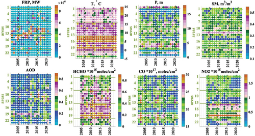
For June, matrix plots for spatial and temporal distribution of the FRP, meteorological parameters (temperature, precipitation, and soil moisture), AOD, and emitted gases (HCHO, CO, and NO₂) are shown in Figure 10. Matrix plots for 4 months (May to August) are shown in Figure S6 (for T, P, SM, FRP, and FC) and Figure S7 (for FRP, AOD, HCHO, CO, and NO₂).

Naturally, the FRP and FC show similar patterns. Before 2010, more fires had been observed in May in central and southern Russia. June looks like a month with the most minor fire activity. Fire activity increases in July in Eastern Europe and Siberia and remains relatively high in August.

Matrix plots show fire activity has increased in Siberia in the last decade. With the temperature growth (especially in May and June) at lower precipitation, northern Siberia (Areas 5–7) has been burning widely and intensively in years 2013 and 2018–2021 in July and August. With those two factors (high T and low P), this area’s increased number of fires can be explained. The increase in AOD nicely follows the burning.

Central China (Area 19) has been burning much less than Eastern Europe, South Russia, and Siberia. Pollutants associated with forest fires are more concentrated in the northeast and south regions than in the west and central regions (Jin et al., 2022). However, the highest AOD, HCHO, CO, and NO₂ values are observed in this area. Possible transport of the long-lived pollutants (HCHO, CO) from Area 19 to Areas 18 and 20 can be seen. For a short-lived NO₂, the concentration in the neighbouring areas with lower economic activity remains low.

Eastern Europe (Area 14) is the second highest in the HCHO area. The NO₂ values are also high in Eastern Europe and central Russia (Areas 8 and 9), where fires happen more often than in China. However, AOD and CO levels are considerably lower than in China (He et al., 2018).

An interesting tendency has been observed for CO. In May and June, CO concentrations have been gradually decreasing during the last two decades. This tendency has been observed for all selected areas. With this, two exceptions also exist in the whole PEEX domain – higher than in neighbouring years’ concentration in June–July 2003 and maximum concentration in August 2021 (Hayasaka, 2021). Those maxima have been explained in Yurganov and Rakitin (2022) by occasional mega-fires, likely due to long-lasting blockages in high-pressure systems (heat waves) and severe droughts.

Although general conclusions can be drawn from matrix plots when operating with the actual values, the high difference in ranges between variables and the contribution of the background values may disturb the analysis. To avoid this and to make variables more closely inter-comparable, the approach described in Sect. 4.4 (scaled anomalies) has been applied. For the FRP (with 0 background value), a logarithm has been taken from the areal average before scaling from 0 to 1. This type of visualisation shows the temporal variation of variables within the areas but makes classifying areas based on the level of pollutants or meteorological conditions impossible.

The matrix plot for scaled anomalies for July is shown in Figure 11 (for all months see Supplement, Figures S8 and S9).

Figure 11. As Figure 10, for scaled anomalies.

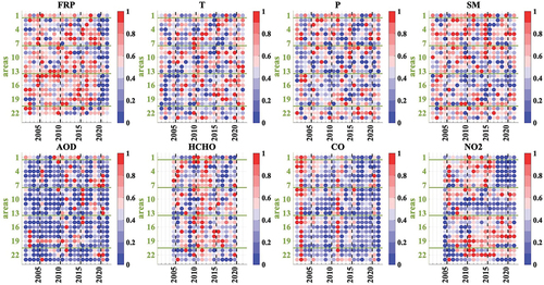
Besides the positive tendency in temperature in northern Siberia, we see a general tendency that temperature is rising in the 2010s, and soil moisture is decreasing in most areas. Interestingly, FRP in 2020–2022 has been lower in a significant part of the PEEX domain (except heavy burning in eastern and north-eastern Siberian Arctic, Areas 6, 7, and 13), while FC has not decreased. This indicates that fires have been smaller in these areas (especially in May), but intensity (energy release) has increased.

A decrease in AOD has been observed in the last two decades, especially in May and June. Maximum AOD in Areas 16–22 correlates well with the strongest fires in Areas 17 and 18 in 2003 (e.g. Huang et al., 2009; Wang et al., 2022; Zhang et al., 2022), which confirms the long-range transport of aerosol particles and emitted long-lived gases. In most of the less polluted areas, a drop in NO₂ was observed in May starting from 2017 and June–July starting from 2018. Opposite, NO₂ is higher in August in the last decade. This month, an increase in the number of fires in Siberia may have contributed to the NO₂ concentration.

5.3.3.2. Correlation of relative and scaled anomalies

To reveal if a dependence exists between meteorological parameters and fire activity and between fire activity, AOD, and emitted gases, we calculated Pearson correlation coefficients (and corresponding p-values) between different parameters, represented by actual values, values above background, anomalies, and relative anomalies. The results are summarised in Table 3.

Table 3. For different domains, correlation coefficients between lnFRP and temperature (T), precipitation (P), soil moisture (SM), AOD, CO, HCHO, NO₂ for actual values (actual), anomalies (anom), relative anomalies (rel. anom), and scaled anomalies (scaled anom). Same after background values (BG) have been removed. Values are replaced with * if the corresponding p-value is >0.05.

		T	P	SM	AOD	CO	HCHO	NO2
Whole domain	actual	*	0.26	*	0.50	0.23	0.41	0.27
	BG removed	−0.39	0.23	0.34	0.47	0.41	0.30	*
	anom	−0.28	*	*	0.41	0.40	0.14	0.25
	rel.anom	0.16	−0.06	−0.10	0.19	0.21	0.21	0.16
	scaled anom	−0.17	−0.07	0.03	0.56	0.30	0.35	0.34
Zones:
SZ (45 º N–55º N)	actual	0.16	*	*	0.34	*	0.26	*
	BG removed	*	*	*	0.34	0.31	0.23	*
	anom	*	−0.27	*	0.31	0.27	0.23	*
	rel.anom	*	−0.27	*	0.33	0.29	0.26	*
	scaled anom	0.02	−0.28	−0.22	0.36	0.34	0.35	0.16
MZ (55 º N–65º N)	actual	0.34	*	−0.43	0.57	*	0.55	0.48
	BG removed	*	*	*	0.54	0.37	0.41	0.31
	anom	*	−0.31	−0.28	0.45	0.40	0.26	0.34
	rel.anom	*	−0.30	−0.28	0.49	0.40	0.30	0.39
	scaled anom	*	−0.31	−0.37	0.64	0.35	0.28	0.40
NZ (65 º N–73º N)	actual	0.73	0.42	−0.74	0.45	*	0.28	0.30
	BG removed	*	0.35	0.32	0.44	*	*	*
	anom	0.36	−0.33	−0.40	0.43	0.29	*	0.24
	rel.anom	*	−0.29	−0.38	0.43	0.26	*	*
	scaled anom	0.40	−0.23	−0.40	0.27	*	*	*
Areas:
Area 1, Scandinavia	actual	0.21	*	−0.48	*	*	0.37	0.15
	BG removed	0.32	−0.35	−0.30	*	0.28	0.31	0.15
	anom	0.32	−0.41	−0.51	*	0.35	0.32	*
	rel.anom	0.32	−0.43	−0.51	*	*	0.37	0.25
	scaled anom	0.46	−0.54	−0.54	*	*	0.47	*
Area 11, Central Siberia	actual	0.24	−0.47	−0.52	0.53	0.29	0.52	0.25
	BG removed	0.45	−0.49	−0.52	0.53	0.38	0.47	0.24
	anom	0.43	−0.56	−0.71	0.53	0.35	0.49	0.19
	rel.anom	0.29	−0.56	−0.71	0.54	0.35	0.58	*
	scaled anom	0.39	−0.43	−0.43	0.58	0.26	0.57	0.36
Area 19, Central China	actual	*	*	−0.45	*	*	*	*
	BG removed	0.26	−0.35	−0.37	*	*	0.65	0.26
	anom	0.24	−0.26	−0.34	0.21	0.02	0.60	0.23
	rel.anom	0.32	*	−0.30	*	*	0.43	*
	scaled anom	0.34	−0.29	−0.27	*	*	0.30	*

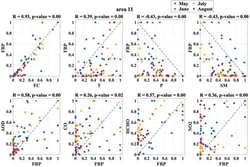
For central Siberia (Area 11), scatter plots for relative anomalies for T, P, SM, and lnFRP, as well as for lnFRP and AOD, CO, HCHO, and NO₂ for the months May–August are shown in Figure 12. Correlation coefficients between variables and corresponding p-values were calculated for the whole summer period (May–August), while markers in the legend allow the separation of data into separate months. Relative anomalies of lnFRP often follow the sign of the T anomaly. Although the correlation between these two variables was not high (R = 0.29), the fraction of the expected responses (ERF) for temperature and lnFRP anomalies is high (68%, wherein 33% of both anomalies are positive, while in 35%, they are negative).

Figure 12. For central Siberia (Area 11), upper panel: scatterplots for lnFC, temperature (T), precipitation (P), and soil moisture (SM) monthly relative anomalies (x-axis) for years 2002–2022 and FRP relative anomalies (y-axis). Lower panel: scatterplots for different combinations of lnFRP relative anomalies (x-axis) and AOD, CO, HCHO, and NO₂ (y-axis) relative anomalies. Pearson correlation coefficient R is given on top of each panel; the p-value is provided. Percentages of points (from the total number of points) are shown in the “expected” quarters (e.g. for precipitation and soil moisture “expected” quarters are sector 90º–180º (T< 0or p < 0, and FRP > 0, coloured light yellow) and sector 270º–360º (T> 0 or p > 0, FRP < 0, coloured light orange); for other variables “expected” quarters are sector 0º–90º (anomalies are positive for both variables, coloured light red) and sector 180º–270º (anomalies are negative for both variables,coloured light blue)). The colour of the dots shows the month (see the legend).

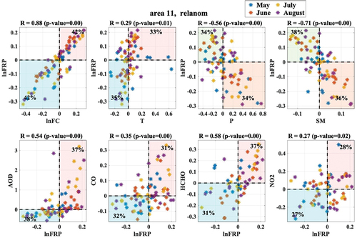
The lnFRP response to precipitation and soil moisture is of the opposite sign. The ERF between lnFRP and precipitation and soil moisture (68% and 74%, respectively) were similar to the ERF between lnFRP and temperature. In contrast, the correlation coefficients between lnFRP relative anomalies and precipitation and soil moisture relative anomalies were considerably higher (−0.56 and −0.71, respectively). For AOD, CO, HCHO, and NO₂, correlation coefficients with lnFRP (0.54, 0.35, 0.58, 0.27, respectively) and ERF (75%, 63%, 68%, and 55%, for AOD, CO, HCHO, and NO₂, respectively) were high.

In Scandinavia (Figure S10) and central China (Figure S11), lnFRP relative anomalies show a similar response to the temperature relative anomalies as in central Siberia. lnFRP response to the precipitation and soil moisture is less clear (−0.43, −0.51) in Scandinavia and even smaller in China (−0.15, −0.30). In Scandinavia, a weaker response of the AOD, CO, HCHO, and NO₂ of lnFRP (0.16, 0.15, 0.37, 0.25, respectively) can be explained by much less intensive forest fires compared to Siberia. In China, where an atmospheric composition is strongly influenced by anthropogenic emissions (e.g. Li et al., 2017; Shen et al., 2019; Tong et al., 2020; Wang et al., 2017; Wang et al., 2022a; Zhang et al., 2022) and biomass burning of croplands and grasses exceed forest fires (Randerson et al., 2012; Xia et al., 2013), no response of CO and NO₂ on lnFRP was revealed. The correlation between the AOD and the lnFRP and HCHO was 0.21 and 0.43, respectively.

For scaled anomalies (Figure 13), correlation coefficients between lnFRP and other variables were improved compared to relative anomalies (Figure 12) in central Siberia for T (from 0.29 to 0.39), and AOD (from −0.54 to −0.58), remained similar for HCHO and slightly lowered for P, SM, and CO.

Figure 13. For central Siberia (Area 11), upper panel: scatterplots of scaled lnFC, T, P, SM (x-axis), and scaled FRP (y-axis). Lower panel: scatterplots scaled FRP (x-axis) and scaled AOD, CO, HCHO, and NO₂ (y-axis). The Pearson correlation coefficient R is shown on top of each panel. The color of each fit shows the month (see the legend).

For the whole PEEX domain (Table 3, Figures S14–S17), the correlation with ln(FRP) scaled anomalies increased compared to relative anomalies from 0.19 to 0.56 for AOD, from 0.21 to 0.30 for CO, from 0.21 to 0.35 for HCHO, from 0.16 to 0.34 for NO₂.

5.4. Trend analysis

As shown in Figure 2, there is a variation in fire activity between the summer months; thus, we performed trend analysis (as in Sect. 4.5) for each month separately and for the whole summer. Statistically significant trends are shown in Figure 14 for the whole PEEX domain (Figure 1, Sect. 2), zones NZ, MZ, and SZ and for Scandinavia, Central Siberia, and China (Areas 1, 11 and 19, respectively).

Figure 14. Decadal trends of FC, FRP, meteorological parameters, AOD, and atmospheric gases for the whole PEEX domain, zones NZ, MZ, and SZ, and Areas 1, 11, and 19. Units are as in Figure 10.

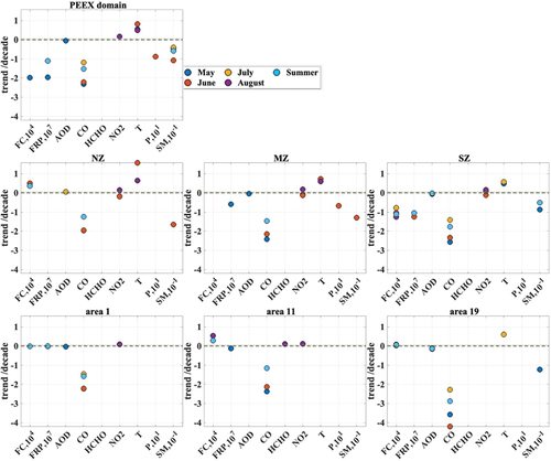
Positive T trends in the NZ in June and August (1.56°C and 0.64°C, respectively) contribute most to the positive T trends in the whole PEEX domain, where, besides June and August, positive T trend in May is also significant. All statistically significant trends of P and SM are negative.

In the PEEX domain, FC is decreasing in May, and the FRP trend is negative also in May and for the whole summer. The decrease in AOD in May addresses the negative trends in FC and FRP.

The decrease in CO concentration, which we discussed in Sect. 5.5.1, is confirmed by the trends analysis. CO trends are negative in May, June, and over summer for all regions; in July in Europe, China, SZ, and the PEEX domain. However, in August, CO trends were not significant in all regions. HCHO trends are not significant in all regions. NO₂ trends are positive in May and negative in June in all zones.

6. Satellite-derived enhancement ratios AOD:CO, AOD:HCHO and AOD:NO₂

To determine AOD:CO, AOD:HCHO, and AOD:NO₂ satellite-derived enhancement ratios (satER) for wildfire emissions, we extracted locations with monthly cumulative FRP above 0 and combined locations based on the land type (as in Figure 1, whole area). To interpret our results, we utilized emission factors from the experimental dataset (Akagi et al., 2011) and emission factors of the IS4FIRES fire information system (Soares et al., 2015; Sofiev et al., 2009). The IS4FIRES coefficients are identified via a top-down approach involving the SILAM atmospheric composition model for estimating the plume dispersion. IS4FIRES-SILAM system utilizes regional emission factors.

We chose three land types from the experimental dataset, savanna, crop residual, and boreal forest, which are close to the land types considered in our study; grass, shrub, crop residual, and boreal forestland types are chosen from the IS4FIRES model. AOD is not available in the experimental and model datasets. Instead, we used PM (particulate matter; PM_2.5 from the experimental dataset and a fire-induced particulate matter PM_FRP, which is a sum of primary and secondary aerosols induced by fires in SILAM) and calculated experimental (expER) and modelled (modER) enhancement ratios. Note that SatER, with units of 1/var_units (AOD is unitless; var_units are units for CO, HCHO, or NO₂), cannot be compared directly to the expER or modER, which are both unitless; moreover, the relation between AOD and PM mass is generally non-linear. However, we can compare the relative distribution of the ERs between land type classes in each dataset (sat, exp, and mod) and compare those results between datasets.

Large territories considered resulted in various conditions within each land-use class. For all matchups (Figure 15), satER AOD:CO is within 0.12 (for Deciduous Needleleaf forest) and 0.18 (for Broadleaf crops). AOD:CO varies between 0.13 and 0.15 for the other land types. However, the standard deviations of satER AOD:CO for all land types are high (0.05–0.13), and all are overlapping. Thus, no statistically significant difference in satER AOD:CO between land types can be reported.

Figure 15. Top panel: AOD:CO ratios of monthly satellite data for pixels with FRP>0 (left); PM_2.5:CO from Akagi et al. (2011) (middle); PM_FRP:CO as in SILAM (right). Middle panel: same for AOD(or PM):HCHO. Lower panel: same for AOD(or PM):NO₂(or NO, NOx).

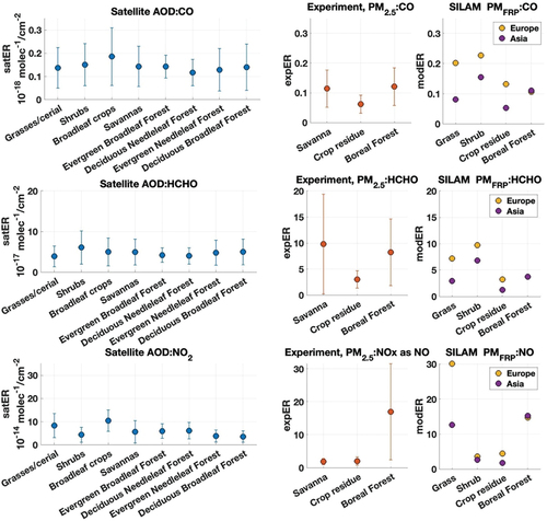
For expER, PM_2.5:CO is decreasing from crop (0.65) to savanna (0.121) and boreal forest (0.123); error bars for three land types are also overlapping, as for satER. SILAM PM_FRP:CO in Asia is close to the experimental dataset for crops and boreal forest, whereas for crops, grass, and shrubs in Europe, the modER is higher (by 0.07–1.2).

SatER AOD: HCHO shows similar to satER AOD:CO distribution, with wider (about two orders of magnitude) compared to AOD:CO spread between the land types. For expER, the AOD:HCHO ratio and spread between land types is also two orders of magnitude wider (from 3.5 for crops to 10 for savanna), with higher standard deviation for savanna and boreal forest. Regional offsets of modER PM_FRP:HCHO are generally of the same order of magnitude as expER and higher for Europe, as it was for modER PM_FRP:CO.

SatER AOD: NO₂ is the lowest for grass (4.2), is around 5 for different types of forests and savannas, and reaches the highest number (5.8) for shrubs. ExpER PM_2.5:NOx ratio for savanna and crop residual is close to each other (2 and 2.5, respectively), while for boreal forest, the ratio is ~8.5 times higher (17); the corresponding standard deviations are high (ca.60–80% of the provided ratios) for all experimental land types. As satER, modER PM(FRP)/NO is higher for grass compared to boreal forests (in Europe).

A common feature has been recognised for all three datasets: AOD(PM):CO and AOD(PM):HCHO ratios for grass are clearly lower than for shrubs. Shrubs, burning more intensively, release more soot and less gas-phase pollutants. For AOD(PM):NOx, the relation between ratios for grass and shrubs is opposite since burning grass releases more nitrogen pollution than burning shrubs (https://escholarship.org/content/qt390342gw/qt390342gw_noSplash_5ecc4d52443cc55eb4f147847a7ef546.pdf, last access 02.11.2023).

In NZ, there is no significant difference in the Ers for grass and shrubs, while in the direction to the south, AOD:CO and AOD:HCHO ER are higher for shrubs (Figure 16). South from 55° N, the highest ER is revealed for broadleaf crops. AOD:NO₂ Ers are approximately twice as high in the SZ for grass, shrubs, savannas, and evergreen needleleaf forests.

Figure 16. For three latitudinal zones (>65°N, 55°N–65°N, <55°N, columns left to right), satER for AOD:CO, AOD:HCHO, AOD:NO₂ (panels top-down).

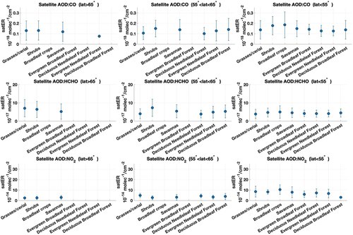
The difference in Ers is statistically significant (error bars are not overlapping) for the low (<0.5) and the high (>0.5) AOD (Figure 17). Since about 90% of AOD values are low (Sogacheva et al., 2020), Ers for low AOD are close to Ers obtained for all AOD ranges. AOD:CO Ers are about three times higher, while AOD:HCHO are about twice higher for the high AOD. For grass and broadleaf crops, AOD:NO₂ Ers are 1.5–2 times higher for the high AOD, while the difference is not significant for other land types.

Figure 17. For different AOD ranges (all AOD, AOD ≤0.5, AOD ≥0.5, columns left to right), satER for AOD:CO, AOD:HCHO, AOD:NO₂ (panels top-down).

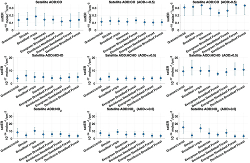
7. Ground-based analysis: OC/BC from AERONET

Wildfires can emit substantial amounts of BC and light-absorbing OC, known as brown carbon (BrC), into the atmosphere. Being emitted, BC can be transported over thousands of kilometers (e.g. May et al., 2023). Since BC and BrC concentrations are not available from satellite data products but can be estimated by using AERONET inversion product, we also included an analysis of light-absorbing carbonaceous aerosols in selected AERONET stations.

A method to estimate columnar black carbon (BC) concentrations from AERONET-retrieved imaginary indices was first suggested by Schuster et al. (2005). This approach was then extended to include the absorption by organic carbon (OC), often called Brown Carbon, in Arola et al. (2011). In their method, the possible influence of dust absorption was essentially excluded with the required minimum threshold for fine mode fraction (FMF). Although this approach has been further developed by Schuster et al. (2016) to include dust absorption, in our study, we used the approach by Arola et al. (2011) and a threshold for FMF of 0.6 to estimate columnar BC over selected AERONET stations covering our area of interest.

We used imaginary indices from the AERONET V3 Level 1.5 inversion product to estimate the columnar BC concentrations. This was done to get better temporal data coverage than from the Level 2 data product, which restricts the good quality measurement for cases when AOD at 440 nm is larger than 0.4. However, we applied an AOD threshold 0.2 at 440 nm to include good-quality data (Sinyuk et al., 2020).

Figure 18 shows the retrieved seasonal mean black carbon column concentration (in mg m⁻²) in May–August for six AERONET sites in the PEEX-relevant domain. Although good temporal data coverage were searched for, there are years of missing or small amounts of data in some stations. These plots show 4-month means and medians, so very strong episodic cases are necessarily smoothed out. For instance, from Figures 10 and 11, it is evident that the record high AOD in the Moscow region (Area 8) was in August 2010, which does not become equally evident in the multi-month data set shown here. However, even with these seasonal plots, substantial inter-annual variability is apparent. Moreover, these results suggest that there would be a clear decreasing trend of BC concentrations in Beijing.

Figure 18. Boxplot of seasonal (May–August) columnar BC concentrations inferred from AERONET measurements for the following sites: Helsinki, Moscow, Yekaterinburg, Tomsk, Yakutsk, and Beijing. Boxplots give the seasonal medians (with 5^th/95^th percentiles) of BC concentrations, and red points provide the mean values in addition. The numbers below the boxes indicate the total number of measurements included in the seasonal means/medians in each year.

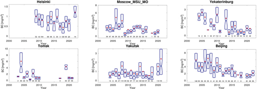
8. Conclusions

The overall goal of this study was to improve an understanding of the effects of forest fires on gas and particle emissions, and how these might change with increasing temperature in the Pan-Eurasian Experiment (PEEX) domain, which covers different vegetation zones (e.g. croplands/grasslands, forest, arctic tundra) of Pan-Eurasia and China. Satellite, modelled, and ground-based data were utilised to find the response of the fire activity on the meteorological parameters (temperature, precipitation, and soil moisture) and response of the AOD and emitted gases (CO, HCHO, and NO₂) on the fire activity.

By utilising 21 years of satellite AOD and emitted gases data, we estimated the background for the AOD and CO, HCHO, and NO₂ concentrations over the PEEX domain. AOD deviates most (0.4–0.5) from the background over Siberia, characterised by the highest fire activity in the PEEX domain. Outside Siberia, a high deviation of the AOD from the background values has been observed in China, where anthropogenic emissions contribute strongly to AOD. CO shows a spatial distribution similar to AOD. HCHO shows a general tendency to increase towards the North. Forest fires in central Siberia can be recognised by the highest (above 3.5 × 10¹⁵ molec/cm²) HCHO anomalies. As with actual values, regions with high anthropogenic pollution can be recognised in the spatial distribution of NO₂ anomalies.

By combining the information on the vegetation type with fire activity, we showed that intra-summer variation of the fire activity depends on the vegetation type, which, in turn, has a latitudinal dependence on, e.g. temperature and precipitation. Cropland/grassland areas are burning predominantly in May and August, which corresponds to seasonality in agricultural activity. Extended Siberian forests are burning mainly in July and August, when the temperature is the highest, while precipitation and soil moisture are the lowest. Siberian fires show closer dependence on anomalies of the meteorological parameters. lnFRP was less sensitive to temperature, precipitation, and soil moisture in the grassland and least sensitive in the cropland zone. Thus, atmospheric composition is more sensitive to biomass-burning events in forest areas than in cropland areas, where the contribution of anthropogenic pollution to the atmosphere is often high. Anomaly data shows that in industrialised areas, high anthropogenic emissions dominate the atmospheric composition and mask the response of aerosols and trace gases to wildfires.

We showed that central China, where anthropogenic activity is high, has been burning much less compared to Eastern Europe, South Russia, and Siberia; however, the highest AOD, HCHO, CO, and NO₂ values are observed in this area. Possible transport of the long-lived pollutants (HCHO, CO) from central China to northern neighbouring areas can be seen. For a short-lived NO₂, the concentration in the neighbouring areas with lower economic activity remains low.

Over the PEEX domain, lnFRP shows a negative correlation to precipitation and soil moisture (−0.28 and −0.30, respectively). The correlation between lnFRP and temperature is positive (0.28) reaching values of 0.4–0.8 over the areas with high FRP. As expected, higher temperatures, lower precipitation, and soil moisture are favourable for a more intensive fire activity.

We showed positive T trends in the NZ in June and August (1.56°C and 0.64°C, respectively); all statistically significant trends of P and SM are negative. This finding may suggest favourable conditions for an increase in fire activity. Indeed, the FC trend is positive; an increase in fire activity in Siberia for the recent years (2019–2022) is also seen on the matrix plots. Over the PEEX domain, FC and FRP trends remain insignificant or negative; a decrease in AOD in May may address those negative trends.

AOD, CO, HCHO, and NO₂ show positive responses on the increased fire activity (correlation coefficients are 0.27, 0.29, 0.33, and 0.29 respectively). AOD, CO, and HCHO responses on the lnFRP are stronger for forest and savannas (tundra). NO₂ response on the lnFRP is stronger for shrubs, broadleaf crops, and savannas. We showed that in May and June, CO concentration has gradually decreased in the last two decades (except for 2021). A trend analysis has confirmed this observed decrease. CO trends are negative in May, June, and over summer for all regions; in July in Europe, China, SZ, and PEEX domain. HCHO trends are not significant in all regions. NO₂ trends are positive in May and negative in June in all zones.

We calculated AOD:CO, AOD:HCHO, and AOD:NO₂ satellite-derived enhancement ratios for wildfire emissions for different land types. To interpret our results, we utilized emission factors from the experimental dataset and emission factors of the IS4FIRES fire information system. A common feature has been recognized for all three datasets: AOD(PM):CO and AOD(PM):HCHO ratios for grass are clearly lower than for shrubs. Shrubs, burning more intensively, release more soot and less gas-phase pollutants. For AOD(PM):NOx, the relation between ratios for grass and shrubs is opposite since burning grass releases more nitrogen pollution than burning shrubs. We showed that AOD:CO and AOD:HCHO emission ratios are increasing towards South and are 2–3 times higher for high (>0.5) AOD. Thus, we show that it is feasible to attempt obtaining emission factors using satellite data. However, it is beyond the scope of this study to provide exact numbers. We find promising results for remote locations with no in-situ data (e.g. Siberian forest), but further work is required to obtain emission factors or inventories to be used in climate models.

We analysed AERONET-based estimates for absorbing carbonaceous aerosols at selected AERONET stations within the PEEX domain. Substantial inter-annual variability in BC concentrations was apparent, probably the most due to the inter-annual variability in fire activities. However, it is to be emphasized that the method we used (Arola et al., 2011) separates BC and BrC absorption and assumes that BC absorbs through the solar spectrum, while BrC has only low absorption in mid-visible but intensifies towards UV wavelengths. On the other hand, some recent studies have highlighted the importance of so-called dark brown carbon emitted by wildfires (e.g. Chakrabarty et al., 2023), which can have significant absorption also in visible wavelengths, in short-visible in particular.

While this study cannot provide improved coefficients to be used in climate models, it points to the observed differences between the responses under different conditions. We show that a complex approach, including analysis of the modelled climate data, atmospheric products retrieved from different satellite instruments, and ground-based products, allows for obtaining a complex picture of the fire activity, its precursors, and consequences for the atmosphere and revealing spatial differences related to the distribution of vegetation types and anthropogenic activity.

Acknowledgements

This study is realised within the frameworks of the PEEX Programme Science Plan as well as with financial support from the Academy of Finland grant No 337549 (Atmosphere and Climate Competence Centre, ACCC).

Data availability statement

Larisa Sogacheva (2023). Satellite-retrieved AOD, CO, HCHO, and NO₂ background over the PEEX domain [Data set]. Finnish Meteorological Institute. https://doi.org/10.23728/FMI-B2SHARE.003652E36B1B4FABA14283DE53C50B61

Disclosure statement

No potential conflict of interest was reported by the author(s).

Supplementary material

Supplemental data for this article can be accessed online at https://doi.org/10.1080/20964471.2024.2316730

Additional information

Notes on contributors

Larisa Sogacheva

Larisa Sogacheva works as a senior scientist at Atmospheric Radiation Group, Atmospheric Research Centre of Eastern Finland, Climate Research Programme, Finnish Meteorological Institute. Her research focuses on satellite remote sensing of aerosols, aerosol products validation and inter-comparison, climate data records. She is a member of Sentinel-3 Next Generation (Optical) Mission Advisory Group (MAG) and vice-chair for AEROSAT

Timo H. Virtanen

Timo H. Virtanen works as a senior scientist at the Finnish Meteorological Institute (Atmospheric Radiation Research Group, Climate Research Programme). His research focuses on satellite remote sensing of atmospheric aerosols, and he is experienced in algorithm development and verification. He has worked on volcanic ash retrieval, observation geometry issues for dual-view satellite instruments, and collocation mismatch uncertainties in satellite retrievals. Recently, he has worked on aerosol-cloud-interactions and atmospheric correction for satellite SIF and XCO2 retrievals

Anu-Maija Sundström

Anu-Maija Sundström works as a senior scientist at Atmospheric Remote Sensing Group, Space and Earth Observation Centre, Finnish Meteorological Institute. Her research focuses on satellite remote sensing of atmospheric composition and aerosols, as well as air quality. She also contributes to several joint training activities by EUMETSAT, Copernicus, and ESA on satellite remote sensing.

Pekka Kolmonen

Pekka Kolmonen, PhD in physics, is a senior research scientist at the Finnish Meteorological Institute, Helsinki, Finland. He has done research on in situ measurement and satellite remote sensing of aerosols. He is concentrating mostly on developing and testing satellite aerosol retrieval algorithms for ESA ATSR2/AATSR/SLSTR, MERIS/OLCI, and OMI instruments. He is involved in aerosol–cloud interaction research. He is developing the atmospheric correction for the ESA FLEX mission.

Mikhail Sofiev

Mikhail Sofiev has worked in the field of atmospheric physics and chemistry concentrating on the development and application of the Eulerian and Lagrangian air pollution models for meso-to-global scales in the troposphere and the stratosphere, as well as operational air quality and accidental release dispersion forecasting. He is the coordinator of development of System for Integrated modeLling of Atmospheric coMposition (SILAM). His specific areas of interest include model development, verification and comparison with measurements, data assimilation, statistical methodology for model validation, analysis of the measurement data, inverse and adjoint dispersion modeling, computer experiments, etc. Compounds of interest are acidifying and toxic pollutants, ozone, radioactive and biological species, and atmospheric aerosols.

Hanna K. Lappalainen

Hanna K. Lappalainen is currently serving as the Pan-Eurasian Experiment (PEEX) Program Secretary General at the University of Helsinki, Institute for Atmospheric and Earth System Research (INAR) in Finland. She also holds the position of coordinator of the Atmosphere and Climate Competence Center (ACCC) Impact Program, and serves as a lead editor of the PEEX Science Plan. She has a long-term experience of coordinating large-scale research projects. In 2005, she received NASA Goddard Team Award EOS-AURA satellite OMI-Team, and in 2015, she was honoured with the Silver Medal from the International Eurasian Academy of Sciences (IEAS). She actively represents Finland in the Sustainable Sustaining Arctic Observing Networks (SAON) Data working group and serves as a national delegate of the International Science Initiative in the Russian Arctic (ISIRA). Additionally, she holds the position of Co-chair of the Arctic-GEOSS-High Mountain-Gold Regions HiMAC, starting from 2020. Dr Lappalainen is an esteemed member of the IEAS Academy and has been since her nomination in December 2016. She also co-leads the “Arctic-boreal Hub” network within the Universities of Arctic and collaborates closely with Academician M. Kulmala. Moreover, she serves on the SIOS Editorial Board and is a member of the SIOS Data Working Group. Lappalainen obtained her Ph.D. from the University of Helsinki, Finland. Her research has primarily focused on the analysis of atmospheric biogenic volatile organic compounds and plant phenology.

Antti Arola

Antti Arola is a Research Professor at the FMI. He is currently leading the Atmospheric Radiation Group at the FMI’s Atmospheric Research Centre of Eastern Finland. He is also Docent (Adj. Prof.) in Remote Sensing at the University of Eastern Finland. He has longstanding experience and expertise on aerosol radiative properties taking advantage of both satellite- and ground-based remote sensing measurements.

References

- Akagi, S. K., Yokelson, R. J., Wiedinmyer, C., Alvarado, M. J., Reid, J. S., Karl, T., Crounse, J. D., & Wennberg, P. O. (2011). Emission factors for open and domestic biomass burning for use in atmospheric models. Atmospheric Chemistry & Physics, 11(9), 4039–4072. https://doi.org/10.5194/acp-11-4039-2011
- Andreae, M. O. (1991). Biomass burning: Its history, use, and distribution and its impact on environmental quality and global climate. In J. S. Levine (Ed.), Global biomass burning: Atmospheric, climatic, and biospheric implications (pp. 3–21). MIT Press.
- Andreae, M. O. (2011). Emission of trace gases and aerosols from biomass burning – an updated assessment. Atmospheric Chemistry & Physics, 19(13), 8523–8546. https://doi.org/10.5194/acp-19-8523-2019
- Andreae, M. O., & Crutzen, P. J. (1997). Atmospheric aerosols: Biogeochemical sources and role in atmospheric chemistry. Science, 276, 1052–1058. https://doi.org/10.1126/science.276.5315.1052
- Andreae, M. O., & Merlet, P. (2001). Emission of trace gases and aerosols from biomass burning. Global Biogeochemical Cycles, 15(4), 955–966. https://doi.org/10.1029/2000GB001382
- Arola, A., Schuster, G., Myhre, G., Kazadzis, S., Dey, S., & Tripathi, S. N. (2011). Inferring absorbing organic carbon content from AERONET data. Atmospheric Chemistry & Physics, 11(1), 215–225. https://doi.org/10.5194/acp-11-215-2011
- Boersma, K. F., Eskes, H. J., Dirksen, R.J., van der A R. J., Veefkind, J. P., Stammes, P., Huijnen, V., Kleipool, Q. L., Sneep, M., Claas, J., Leitão, J., Richter, A., Zhou, Y., & Brunner, D. (2011). An improved tropospheric NO2 column retrieval algorithm for the Ozone Monitoring Instrument. Atmospheric Measurement Techniques, 4, 1905–1928. https://doi.org/10.5194/amt-4-1905-2011
- Boersma, K. F., Eskes, H. J., Veefkind, J. P., Brinksma, E. J., van der A, J. R. Sneep, M., van den Oord, G. H. J., Levelt, P. F., Stammes, P., Gleason, J. F., & Bucsela, E. J. (2007). Near-real time retrieval of tropospheric NO2 from OMI. Atmospheric Chemistry & Physics, 7, 2103–2118. https://doi.org/10.5194/acp-7-2103-2007
- Boersma, K. F., Jacob, D. J., Bucsela, E. J., Perring, A. E., Dirksen, R., van der A, J. R. Yantosca, R. M., Park, R. J., Wenig, M. O., Bertram, T. H., & Cohen, R. C. (2008). Validation of OMI tropospheric NO2 observations during INTEX-B and application to constrain NOx emissions over the eastern United States and Mexico. Atmospheric Environment, 42(19), 4480–4497. https://doi.org/10.1016/j.atmosenv.2008.02.004
- Bondur, V. G., Gordo, K. A., Voronova, O. S., Zima, A. L., & Feoktistova, N. V. (2023). Intense wildfires in Russia over a 22-year period according to satellite data. Fire, 6, 99. https://doi.org/10.3390/fire6030099
- Chakrabarty, R. K., Shetty, N. J., Thind, A. S., Beeler, P., Sumlin, B. J., Zhang, C., Liu, P., Wagner, K., Adachi, N. L., Schwarz, J. P., Ahern, A., Sedlacek, A., III, Lambe, J., Daube, A., Lyu, C., Liu, M., Herndon, C., Onasch, S., B, T., & Mishra, R. (2023). Shortwave absorption by wildfire smoke dominated by dark brown carbon. Nature Geoscience, 16(8), 683–688. https://doi.org/10.1038/s41561-023-01237-9
- Chen, Y., & Bond, T. C. (2010). Light absorption by organic carbon from wood combustion. Atmospheric Chemistry & Physics, 10, 1773–1787. https://doi.org/10.5194/acp-10-1773-2010
- Chubarova, N., Nezval’, Y., Sviridenkov, I., Smirnov, A., & Slutsker, I. (2012, summer). Smoke aerosol and its radiative effects during extreme fire event over Central Russia in summer 2010. Atmospheric Measurement Techniques, 5(3), 557–568. https://doi.org/10.5194/amt-5-557-2012
- Compernolle, S., Verhoelst, T., Pinardi, G., Granville, J., Hubert, D., Keppens, A., Niemeijer, S., Rino, B., Bais, A., Beirle, S., Boersma, F., Burrows, J. P., De Smedt, I., Eskes, H., Goutail, F., Hendrick, F., Lorente, A., Pazmino, A. … Lambert, J.-C. (2020). Validation of aura-OMI QA4ECV NO2 climate data records with ground-based DOAS networks: The role of measurement and comparison uncertainties. Atmospheric Chemistry & Physics, 20(13), 8017–8045. https://doi.org/10.5194/acp-20-8017-2020
- Crutzen, P. J., & Andreae, M. O. (1990). Biomass burning in the tropics: Impact on atmospheric chemistry and biogeochemical cycles. Science, 250(4988), 1669–1678. https://doi.org/10.1126/science.250.4988.1669
- Deeter, M., Francis, G., Gille, J., Mao, D., Martínez-Alonso, S., Worden, H., Ziskin, D., Drummond, J., Commane, R., Diskin, G., & McKain, K. (2022). The MOPITT version 9 CO product: Sampling enhancements and validation. Atmospheric Measurement Techniques, 15(8), 2325–2344. https://doi.org/10.5194/amt-15-2325-2022
- de Groot, W. J., Cantin, A. S., Flannigan, M. D., Soja, A. J., Gowman, L. M., & Newbery, A. (2013). A comparison of Canadian and Russian boreal forest fire regimes. Forest Ecology and Management, 294, 23–34. https://doi.org/10.1016/j.foreco.2012.07.033
- de Leeuw, G., Fan, C., Li, Z., Dong, J., Li, Y., Ou, Y., & Zhu, S. (2022). Spatiotemporal variation and provincial scale differences of the AOD across China during 2000–2021. Atmospheric Pollution Research, 13(4), 101359. ISSN 1309-1042. https://doi.org/10.1016/j.apr.2022.101359
- Denman, K. L., Brasseur, A., Chidthaisong, A., Ciais, P., Cox, P. M., Dickinson, R. E., Hauglustaine, D., Heinze, C., Holland, E., Jacob, D., Lohmann, U., Ramachandran, S., da Silva Dias, P. L., Wofsy, S. C., & Zhang, X.: Couplings between changes in the climate system and biogeochemistry, in: climate change 2007: the physical science basis, contribution of working group i to the fourth assessment report of the intergovernmental panel on climate change, Cambridge University Press, ISBN 978-0521705967, (2007).
- de Smedt, I., Pinardi, G., Vigouroux, C., Compernolle, S., Bais, A., Benavent, N., Boersma, F., Chan, K.-L., Donner, S., Eichmann, K.-U., Hedelt, P., Hendrick, F., Irie, H., Kumar, V., Lambert, J.-C., Langerock, B., Lerot, C., Liu, C. … Van Roozendael, M. (2021). Comparative assessment of TROPOMI and OMI formaldehyde observations and validation against MAX-DOAS network column measurements. Atmospheric Chemistry & Physics, 21(16), 12561–12593. https://doi.org/10.5194/acp-21-12561-2021
- Eck, T. F., Holben, B. N., Reid, J. S., Dubovik, O., Smirnov, A., O’Neill, N. T., Slutsker, I., & Kinne, S. (1999). Wavelength dependence of the optical depth of biomass burning, urban, and desert dust aerosol. Journal of Geophysical Research, 104(D24), 31333–31350. https://doi.org/10.1029/1999JD900923
- Edwards, D. P., Emmons, L. K., Hauglustaine, D. A., Chu, A., Gille, J. C., Kaufman, Y. J., Petron, G., Yurganov, L. N., Giglio, L., Deeter, M. N., Yudin, V., Ziskin, D. C., Warner, J., Lamarque, J.-F., Francis, G. L., Ho, S. P., Mao, D., Chen, J., Grechko, E. I., & Drummond, J. R. (2004). Observations of carbon monoxide and aerosols from the terra satellite: Northern Hemisphere variability. Journal of Geophysical Research, 109(D24), D24202. https://doi.org/10.1029/2004JD004727
- Elansky, N., Mokhov, I., Belikov, I., Berezina, E., Elokhov, A., Ivanov, V., Pankratova, N., Postylyakov, O., Safronov, A., Skorokhod, A., & Shumsky, R. (2011). Gas composition of the surface air in Moscow during the extreme summer of 2010. Doklady Earth Sciences, 437(1), 357–362. https://doi.org/10.1134/S1028334X11030020
- Elvidge, C. D., Zhizhin, M., Hsu, F.-C., & Baugh, K. E. (2013). VIIRS nightfire: Satellite pyrometry at night. Remote Sensing, 5(9), 4423–4449. https://doi.org/10.3390/rs5094423
- Fokeeva, E., Safronov, A., Rakitin, V., Yurganov, L., Grechko, E., & Shumskii, R. (2011). Investigation of the 2010 July–August fires impact on carbon monoxide atmospheric pollution in Moscow and its outskirts, estimating of emissions. Izvestiya, Atmospheric and Oceanic Physics, 47(6), 682–698. https://doi.org/10.1134/S0001433811060041
- Frédéric, A., Hugh, E., Mollicone, D., & Beuchle, R. (2008). The effect of climate anomalies and human ignition factor on wildfires in Russian boreal forests. Philosophical Transactions of the Royal Society of London, B363(1501), 2329–2337. https://doi.org/10.1098/rstb.2007.2203
- Freeborn, P. H., Wooster, M. J., & Roberts, G. (2011). Addressing the spatiotemporal sampling design of MODIS to provide estimates of the fire radiative energy emitted from Africa. Remote Sensing of Environment, 115(2), 475–489. https://doi.org/10.1016/j.rse.2010.09.017
- Freeborn, P. H., Wooster, M. J., Roy, D. P., & Cochrane, M. A. (2014). Quantification of MODIS fire radiative power (FRP) measurement uncertainty for use in satellite-based active fire characterization and biomass burning estimation. Geophysical Research Letters, 41(6), 1988–1994. https://doi.org/10.1002/2013GL059086
- Gatebe, C., Ichoku, C., Poudyal, R., Roman, M. O., & Wilcox, E. (2014). Surface albedo darkening from wildfires in northern sub-saharan Africa. Environmental Research Letters, 9(6), 065003. https://doi.org/10.1088/1748-9326/9/6/065003
- Giglio, L., Descloitres, J., Justice, C. O., & Kaufman, Y. (2003). J.: An enhanced contextual fire detection algorithm for MODIS. Remote Sensing of Environment, 87(2–3), 273–282. https://doi.org/10.1016/S0034-4257(03)00184-6
- Giglio, L., Schroeder, W., & Justice, C. O. (2016). The collection 6 MODIS active fire detection algorithm and fire products. Remote Sensing of Environment, 178, 31–41. https://doi.org/10.1016/j.rse.2016.02.054
- Giles, D. M., Sinyuk, A., Sorokin, M. G., Schafer, J. S., Smirnov, A., Slutsker, I., Eck, T. F., Holben, B. N., Lewis, J. R., Campbell, J. R., Welton, E. J., Korkin, S. V., & Lyapustin, A. I. (2019). Advancements in the Aerosol Robotic Network (AERONET) version 3 database – automated near-real-time quality control algorithm with improved cloud screening for sun photometer aerosol optical depth (AOD) measurements. Atmospheric Measurement Techniques, 12(1), 169–209. https://doi.org/10.5194/amt-12-169-2019
- Gilman, J. B., Lerner, B. M., Kuster, W. C., Goldan, P. D., Warneke, C., Veres, P. R., Roberts, J. M., de Gouw, J. A., Burling, I. R., & Yokelson, R. J. (2015). Biomass burning emissions and potential air quality impacts of volatile organic compounds and other trace gases from fuels common in the US. Atmospheric Chemistry & Physics, 15(24), 13915–13938. https://doi.org/10.5194/acp-15-13915-2015
- Golitsyn, G. S., Gorchakov, G. I., Grechko, E. I., Semoutnikova, E. G., Rakitin, V. S., Fokeeva, E. V., Karpov, A. V., Kurbatov, G. A., Baikova, E. S., & Safrygina, T. P. (2012). Extreme carbon monoxide pollution of the atmospheric boundary layer in Moscow region in the summer of 2010. Doklady Earth Sciences, 441(2), 1666–1672. https://doi.org/10.1134/S1028334X11120014
- González Abad, G., Liu, X., Chance, K., Wang, H., Kurosu, T. P., & Suleiman, R. (2015). Updated Smithsonian Astrophysical Observatory Ozone Monitoring Instrument (SAO OMI) formaldehyde retrieval. Atmospheric Measurement Techniques, 8, 19–32. https://doi.org/10.5194/amt-8-19-2015
- Gonzi, S., Palmer, P. I., Barkley, M. P., De Smedt, I., & Van Roozendael, M. (2011). Biomass burning emission estimates inferred from satellite column measurements of HCHO: Sensitivity to co-emitted aerosol and injection height. Geophysical Research Letters, 38(14), L14807. https://doi.org/10.1029/2011GL047890
- Grebner, D. L., Bettinger, P., & Siry, J. (2013). Introduction to forestry and natural resources. Academic Press.
- Greene, C. A., Thirumalai, K., Kearney, K. A., Delgado, J. M., Schwanghart, W., Wolfenbarger, N. S., Thyng, K. M., Gwyther, D. E., Gardner, A. S., & Blankenship, D. D. (2019). The climate data toolbox for MATLAB. Geochemistry Geophysics Geosystems, 20(7), 3774–3781. https://doi.org/10.1029/2019GC008392
- Griffin, D., McLinden, C. A., Dammers, E., Adams, C., Stockwell, C. E., Warneke, C., Bourgeois, I., Peischl, J., Ryerson, T. B., Zarzana, K. J., Rowe, J. P., Volkamer, R., Knote, C., Kille, N., Koenig, T. K., Lee, C. F., Rollins, D., Rickly, P. S. … Makar, P. (2021). Biomass burning nitrogen dioxide emissions derived from space with TROPOMI: Methodology and validation. Atmospheric Measurement Techniques, 14(12), 7929–7957. https://doi.org/10.5194/amt-14-7929-2021
- Groisman, P., & Soja, A. J. (2009). Ongoing climatic change in Northern Eurasia: Justification for expedient research. Environmental Research Letters, 4(4), 045002. 10.1088/1748-9326/4/4/045002
- Hall, J. V., Argueta, F., Zubkova, M., Chen, Y., Randerson, J. T., & Giglio, L. 2024. GloCAB: global cropland burned area from mid-2002 to 2020. Earth System Science Data discussion, 16, 867–885. 10.5194/essd-16-867-2024
- Hall, J. V., Zibtsev, S. V., Giglio, L., Skakun, S., Myroniuk, V., Zhuravel, O., Goldammer, J. G., & Kussul, N. (2021). Environmental and political implications of underestimated cropland burning in Ukraine. Environmental Research Letters, 16(6), 064019. https://doi.org/10.1088/1748-9326/abfc04
- Halofsky, J. E., Peterson, D. L., & Harvey, B. J. (2020). Changing wildfire, changing forests: The effects of climate change on fire regimes and vegetation in the Pacific Northwest, USA. Fire Ecology, 16, 4. https://doi.org/10.1186/s42408-019-0062-8
- Hawbaker, T. J., Radeloff, V. C., Syphard, A. D., Zhu, Z., & Stewart, S. I. (2008). Detection rates of the MODIS active fire product in the United States. Remote Sensing of Environment, 112(5), 2656–2664. ISSN 0034-4257. https://doi.org/10.1016/j.rse.2007.12.008
- Hayasaka, H. (2021). Rare and extreme wildland fire in Sakha in 2021. Atmosphere, 12(12), 1572. https://doi.org/10.3390/atmos12121572
- He, Q., Geng, F., Li, C., Mu, H., Zhou, G., Liu, X., Gao, W., Wang, Y., & Cheng, T. (2018). Long-term variation of satellite-based PM2.5 and influence factors over East China. Scientific Report, 8(1), 11764. https://doi.org/10.1038/s41598-018-29366-x
- He, Q., Qin, K., Cohen, J. B., Loyola, D., Li, D., Shi, J., & Xue, Y. (2020). Spatially and temporally coherent reconstruction of tropospheric NO2 over China combining OMI and GOME-2B measurements. Environmental Research Letters, 15(12), 125011. https://doi.org/10.1088/1748-9326/abc7df
- Holben, B. N., Eck, T. F., Slutsker, I., Tanré, D., Buis, J. P., Setzer, A., Vermote, E., Reagan, J. A., Kaufman, Y., Nakajima, T., Lavenu, F., Jankowiak, I., & Smirnov, A. (1998). AERONET — a federated instrument network and data archive for aerosol characterization. Remote Sensing of Environment, 66(1), 1–16. https://doi.org/10.1016/S0034-4257(98)00031-5
- Huang, S., Siegert, F., Goldammer, J. G., & Sukhinin, A. I. (2009). Satellite-derived 2003 wildfires in southern Siberia and their potential influence on carbon sequestration. International Journal of Remote Sensing, 30(6), 1479–1492. https://doi.org/10.1080/01431160802541549
- Huemmrich, K. F., Gamon, J. A., Tweedie, C. E., Campbell, P. K. E., Landis, D. R., & Middleton, E. M. (2013). Arctic tundra vegetation functional types based on photosynthetic physiology and optical properties. IEEE Journal of Selected Topics in Applied Earth Observations & Remote Sensing, 6(2), 265–275. https://doi.org/10.1109/JSTARS.2013.2253446
- Hugelius, G., Loisel, J., Chadburn, S., Jackson, R. B., Jones, M., MacDonald, G., Marushchak, M., Olefeldt, D., Packalen, M., Siewert, M. B., Treat, C., Turetsky, M., Voigt, C., & Yu, Z. (2020). Large stocks of peatland carbon and nitrogen are vulnerable to permafrost thaw. Proceedings of the National Academy of Sciences U S A, 117(34), 20438–20446. https://doi.org/10.1073/pnas.1916387117
- Huijnen, V., Flemming, J., Kaiser, J. W., Inness, A., Leitao, J., Heil, A., Eskes, H. J., Schultz, M. G., Benedetti, A., Hadji-Lazaro, J., Dufour, G., & Eremenko, M. (2012). Hindcast experiments of tropo-spheric composition during the summer 2010 fires over western Russia. Atmospheric Chemistry & Physics, 12(9), 4341–4364. https://doi.org/10.5194/acp-12-4341-2012
- Ichoku, C., Giglio, L., Wooster, M. J., & Remer, L. A. (2008). Global characterization of biomass-burning patterns using satellite measurements of fire radiative energy. Remote Sensing of Environment, 112(6), 2950–2962. https://doi.org/10.1016/j.rse.2008.02.009
- Ichoku, C., Kahn, R. A., & Chin, M. (2012). Satellite contributions to the quantitative characterization of biomass burning for climate modeling. Atmospheric Research, 111, 1–28. https://doi.org/10.1016/j.atmosres.2012.03.007
- Ichoku, C., & Kaufman, Y. (2005). J.: A method to derive smoke emission rates from MODIS fire radiative energy measurements. IEEE Transactions on Geoscience & Remote Sensing, 43(11), 2636–2649. https://doi.org/10.1109/TGRS.2005.857328
- Innes, J. L., Beniston, M., & Verstraete, M. M. (2000). Biomass burning and its inter-relationship with the climate system. Kluwer Acad.
- Jaffe, D., Bertschi, I., Jaegle, L., Novelli, P., Reid, J. S., Tanimoto, H., Vingarzan, R., & Westphal, D. L. (2004). Long-range transport of Siberian biomass burning emissions and impact on surface ozone in western North America. Geophysical Research Letters, 31(16), L16106. https://doi.org/10.1029/2004GL020093
- Jin, Q. F., Wang, W. W., Zheng, W. X., Innes, J. L., Wang, G. Y., & Guo, F. T. (2022). Dynamics of pollutant emissions from wildfires in China. Journal of Environmental Management, 318, 115499. https://doi.org/10.1016/j.jenvman.2022.115499
- Johnson, M. S., Strawbridge, K., Knowland, K. E., Keller, C., & Travis, M. (2021). Long-range transport of Siberian biomass burning emissions to North America during FIREX-AQ. Atmospheric Environment, 252, 118241. https://doi.org/10.1016/j.atmosenv.2021.118241
- Jones, M. W., Abatzoglou, J. T., Veraverbeke, S., Andela, N., Lasslop, G., Forkel, M., Smith, A. J. P., Burton, C., Betts, R. A., van der Werf, G. R., Sitch, S., Canadell, J. G., Santín, C., Kolden, C., Doerr, S. H., & Le Quéré, C. (2022). Global and regional trends and drivers of fire under climate change. Review of Geophysics, 60(3), e2020RG000726. https://doi.org/10.1029/2020RG000726
- Jung, J. S., & Kang, J. H. (2021). Postharvest burning of crop residues in home stoves in a rural site of Daejeon, Korea: Its impact to atmospheric carbonaceous aerosol. Atmosphere, 12, 257. https://doi.org/10.3390/atmos12020257
- Justice, C. O., Giglio, L., Korontzi, S., Owens, J., Morisette, J. T., Roy, D., Descloitres, J., Alleaume, S., Petitcolin, F., & Kaufman, Y. (2002). The MODIS fire products. Remote Sensing of Environment, 83(1–2), 244–262. https://doi.org/10.1016/S0034-4257(02)00076-7
- Kaufman, Y. (2002). The MODIS fire products. Remote Sensing of Environment, 83(1–2), 244–262. https://doi.org/10.1016/S0034-4257(02)00076-7
- Kim, J.-S., Kug, J.-S., Jeong, S.-J., Park, H., & Gabriela Schaepman-Strub, G. (2020). Arctic oscillation–induced temperature increase drives earlier snow melting and fire activity over southeastern Siberia. Science Advances, 6(2), eaax3308. https://doi.org/10.1126/sciadv.aax3308
- Kramer, L. J., Leigh, R. J., Remedios, J. J., & Monks, P. S. (2008). Comparison of OMI and ground-based in situ and MAX-DOAS measurements of tropospheric nitrogen dioxide in an urban area. Journal of Geophysical Research, 113(D16), D16S39. https://doi.org/10.1029/2007JD009168
- Krotkov, N. A., Lamsal, L. N., Celarier, E. A., Swartz, W. H., Marchenko, S. V., Bucsela, E. J., Chan, K. L., Wenig, M., & Zara, M. (2017). The version 3 OMI NO2 standard product. Atmospheric Measurement Techniques, 10, 3133–3149. https://doi.org/10.5194/amt-10-3133-2017 9
- Kulmala, M., Lappalainen, H. K., Petäjä, T., Kurten, T., Kerminen, V.-M., Viisanen, Y., Hari, P., Sorvari, S., Bäck, J., Bondur, V., Kasimov, N., Kotlyakov, V., Matvienko, G., Baklanov, A., Guo, H. D., Ding, A., Hansson, H.-C., & Zilitinkevich, S. (2015). Introduction: The Pan-Eurasian experiment (PEEX) – multidisciplinary, multiscale and multicomponent research and capacity-building initiative. Atmospheric Chemistry & Physics, 15(22), 13085–13096. https://doi.org/10.5194/acp-15-13085-2015
- Lappalainen, H. K., Kerminen, V.-M., Petäjä, T., Kurten, T., Baklanov, A., Shvidenko, A., Bäck, J., Vihma, T., Alekseychik, P., Andreae, M. O., Arnold, S. R., Arshinov, M., Asmi, E., Belan, B., Bobylev, L., Chalov, S., Cheng, Y., Chubarova, N. … Kulmala, M. (2016). Pan-Eurasian experiment (peex): towards a holistic understanding of the feedbacks and interactions in the land–atmosphere–ocean–society continuum in the northern Eurasian region. Atmospheric Chemistry & Physics, 16(22), 14421–14461. https://doi.org/10.5194/acp-16-14421-2016
- Lappalainen, H. K., Petäjä, T., Kujansuu, J., Kerminen, V.-M., Shvidenko, A., Bäck, J., Vesala, T., Vihma, T., de Leeuw, G., Lauri, A., Ruuskanen, T., Flint, M., Zaitseva, N., Spracklen, M., Arshinov, D., Lihavainen, S., Arnold, S., Juhola, H. … Kulmala, M. (2014). Pan-Eurasian Experiment (PEEX) – a research initiative meeting the grand challenges of the changing environment of the northern Pan-Eurasian arctic-boreal areas. J Geography Environment Sustainability, 7(2), 13–48. https://doi.org/10.24057/2071-9388-2014-7-2-13-48
- Lappalainen, H. K., Petäjä, T., Vihma, T., Räisänen, J., Baklanov, A., Chalov, S., Esau, I., Ezhova, E., Leppäranta, M., Pozdnyakov, D., Pumpanen, J., Andreae, M. O., Arshinov, M., Asmi, E., Bai, J., Bashmachnikov, I., Belan, B., Bianchi, F. … Kulmala, M. (2022). Overview: Recent advances in the understanding of the northern Eurasian environments and of the urban air quality in China – a pan-Eurasian experiment (PEEX) programme perspective. Atmospheric Chemistry & Physics, 22, 4413–4469. https://doi.org/10.5194/acp-22-4413-2022
- Laumbach, R. J., & Kipen, H. M. (2012). Respiratory health effects of air pollution: Update on biomass smoke and traffic pollution. The Journal of Allergy and Clinical Immunology, 129(1), 3–11. ISSN 0091-6749. https://doi.org/10.1016/j.jaci.2011.11.021
- Lavoué, D., Liousse, C., Cachier, H., Stocks, B., & Goldammer, J. (2000). Modeling of carbonaceous particles emitted by boreal and temperate wildfires at northern latitudes. Journal of Geophysical Research: Atmospheres, 105(D22), 26871–26890. https://doi.org/10.1029/2000JD900180
- Leino, K., Riuttanen, L., Nieminen, T., Dal Maso, M., Väänänen, R., Pohja, T., Keronen, P., Jarvi, L., Aalto, P., Virkkula, A., Kerminen, V.-M., Petaja, T., & Kulmala, M. (2014). Biomass-burning smoke episodes in Finland from eastern European wildfires. Boreal Environment Research, 19, 275–292. https://helda.helsinki.fi/server/api/core/bitstreams/8729c483-9866-49e4-a647-9cfdcefdab41/content
- Lemprière, T. C., Kurz, W. A., Hogg, E. H., Schmoll, C., Rampley, G. J., Yemshanov, D., McKenney, D. W., Gilsenan, R., Beatch, A., Blain, D., Bhatti, J. S., & Krcmar, E. (2013). Canadian boreal forests and climate change mitigation. Environmental Reviews, 21(4), 293–321. https://doi.org/10.1139/er-2013-0039
- Levelt, P. F., Oord, G. H. J., van den Dobber, M. R., Mälkki, A., Visser, H., Vries, J., de Stammes, P., Lundell, J., & Saari, H. (2006). The ozone monitoring instrument. IEEE Transactions on Geoscience and Remote Sensing, 44(5), 1093–1101. https://doi.org/10.1109/TGRS.2006.872333
- Liao, J., Wolfe, G. M., Hannun, R. A., Clair, J. M. S., Hanisco, T. F., Gilman, J., Lamplugh, A., Selimovic, V., Diskin, G. S., Nowak, J. B., Halliday, H., DiGangi, J. P., Hall, S. R., Ullmann, K., Holmes, C. D., Fite, C., Agastra, A., Ryerson, T. B. … Hornbrook, R. S. (2022). Brown. In eds S., Womack, C., Robinson, M., Washenfelder, R., Veres, P, & Neuman, J., A.: Formaldehyde evolution in US wildfire plumes during the fire influence on regional to Global Environments and air quality experiment (FIREX-AQ), atmospheric chemistry and physics. https://doi.org/10.5194/acp-21-18319-2021
- Li, M., Liu, H., Geng, G., Hong, C., Liu, F., Song, Y., Tong, D., Zheng, B., Cui, H., Man, H., Zhang, Q., & He, K. (2017). Anthropogenic emission inventories in China: A review. National Science Review, 4(6), 834–866. https://doi.org/10.1093/nsr/nwx150
- Lin, S., Huang, X., Gao, J., & Ji, J. (2021). Extinction of Wood Fire: A Near-Limit Blue Flame Above Hot Smoldering Surface. Fire Technology, 58(1), 415–434. https://doi.org/10.1007/s10694-021-01146-6
- Liu, C., Beirle, S., Butler, T., Liu, J., Hoor, P., Jöckel, P., Penning de Vries, M., Pozzer, A., Frankenberg, C., Lawrence, M. G., Lelieveld, J., Platt, U., & Wagner, T. (2011). Application of SCIAMACHY and MOPITT CO total column measurements to evaluate model results over biomass burning regions and Eastern China. Atmospheric Chemistry & Physics, 11, 6083–6114. https://doi.org/10.5194/acp-11-6083-2011
- Liu, Y., Scott, G., & Warren, H. (2014). Wildland fire emissions, carbon, and climate: Wildfire–climate interactions. Forest Ecology and Management, 317, 80–96. https://doi.org/10.1016/j.foreco.2013.02.020
- Li, F., Zhang, X., Kondragunta, S., & Csiszar, I. (2018). Comparison of fire radiative power estimates from VIIRS and MODIS observations. Journal of Geophysical Research: Atmosphere, 123(9), 4545–4563. https://doi.org/10.1029/2017JD027823
- Lu, Z., & Sokolik, I. N. (2018). The impacts of smoke emitted from Boreal Forest Wildfires on the High Latitude Radiative Energy Budget—A case study of the 2002 Yakutsk Wildfires. Atmosphere, 9, 410. https://doi.org/10.3390/atmos9100410
- Mack, M. C., Walker, X. J., Johnstone, J. F., Alexander, H. D., Melvin, A. M., Jean, M., & Miller, S. N. (2021). Carbon loss from boreal forest wildfires offset by increased dominance of deciduous trees. Science, 372(6539), 280–283. https://doi.org/10.1126/science.abf390
- Mahowald, N. M., Artaxo, P., Baker, A. R., Jickells, T. D., Okin, G. S., Randenson, J. T., & Townsend, A. R. (2005). Impacts of biomass burning emissions and land use change on Amazonian atmospheric phosphorus cycling and deposition. Global Biogeochemical Cycles, 19(4), GB4030. https://doi.org/10.1029/2005GB002541
- Marbach, T., Beirle, S., Liu, C., Platt, U., & Wagner, T.: Biomass burning emissions from satellite observations: Synergistic use of formaldehyde (HCHO), fire counts, and surface temperature, Proc. SPIE 7089, Remote Sensing of Fire: Science and Application, 70890J, https://doi.org/10.1117/12.793654. (2008).
- Markowicz, K. M., Chilinski, M. T., Lisok, J., Zawadzka, O., Stachlewska, I. S., Janicka, L., Rozwadowska, A., Makuch, P., Pakszys, P., Zielinski, T., Petelski, T., Posyniak, M., Pietruczuk, A., Szkop, A., & Westphal, D. L. (2016). Study of aerosol optical properties during long-range transport of biomass burning from Canada to Central Europe. Journal of Aerosol Sciences 101, 156–173. inJuly 2013. https://doi.org/10.1016/j.jaerosci.2016.08.006.
- May, N. W., Bernays, N., Farley, R., Zhang, Q., & Jaffe, D. A. (2023). Intensive aerosol properties of boreal and regional biomass burning aerosol at Mt. Bachelor observatory: Larger and black carbon (BC)-dominant particles transported from Siberian wildfires. Atmospheric Chemistry & Physics, 23, 2747–2764. https://doi.org/10.5194/acp-23-2747-2023
- Meinander, O., Kontu, A., Kouznetsov, R., & Sofiev, M. (2020). Snow samples combined with long-range transport modeling to reveal the origin and temporal variability of black carbon in seasonal snow in Sodankylä (67°N. Frontiers in Earth Sciences, Cryospheric Sciences, 8. https://doi.org/10.3389/feart.2020.00153
- Mielonen, T., Portin, H., Komppula, M., Leskinen, A., Tamminen, J., Ialongo, I., Hakkarainen, J., Lehtinen, K., & Arola, A. (2012). Biomass burning aerosols observed in EasternFinland during the Russian wildfires in summer 2010 –part 2. Remote Sensing of Atmospheric Environment, 47, 279–287. https://doi.org/10.1016/j.atmosenv.2011.07.016
- MOPITT user guide. 2018. https://www2.acom.ucar.edu/sites/default/files/documents/v8_users_guide_201812.pdf, last access 25.08.2023.
- Ngoc Trieu, T. T., Morino, I., Uchino, O., Tsutsumi, Y., Izumi, T., Sakai, T., Shibata, T., Ohyama, H., & Nagahama, T. (2023, April 1). Long-range transport of CO and aerosols from Siberian biomass burning over northern Japan during 18-20 May 2016. Environmental Pollutions, 322, 121129. https://doi.org/10.1016/j.envpol.2023.121129
- Oh, H. R., Ho, C. H., Kim, J., Chen, D., Lee, S., Choi, Y. S., Chang, L. S., & Song, C. K. (2015). Long-range transport of air pollutants originating in China: A possible major cause of multi-day high-PM10 episodes during cold season in Seoul, Korea. Atmospheric Environment, 109, 23–30. https://doi.org/10.1016/j.atmosenv.2015.03.005
- Paris, J.-D., Stohl, A., Nédélec, P., Arshinov, M. Y., Panchenko, M. V., Shmargunov, V. P., Law, K. S., Belan, B. D., & Ciais, P. (2009). Wildfire smoke in the Siberian Arctic in summer: Source characterization and plume evolution from airborne measurements. Atmospheric Chemistry & Physics, 9, 9315–9327. https://doi.org/10.5194/acp-9-9315-2009
- PEEX science plan, https://www.atm.helsinki.fi/peex/images/PEEX_Science_Plan.pdf, last access 25.08.2023.
- Péré, J. C., Mallet, M., Bessagnet, B., & Pont, V. (2009). Evidence of the aerosol core-shell mixing state over Europe during the heat wave of summer 2003 by using CHIMERE simulations and AERONET inversions. Geophysical Research Letters, 36(9), L09807. https://doi.org/10.1029/2009GL037334
- Petäjä, T., Ganzei, K. S., Lappalainen, H. K., Tabakova, K., Makkonen, R., Räisänen, J., Chalov, S., Kulmala, M., Zilitinkevich, S., Baklanov, P. Y., Shakirov, R. B., Mishina, N. V., Egidarev, E. G., & Kondrat’ev, I. I. (2021). Research agenda for the Russian far east and utilization of multi-platform comprehensive environmental observations in. International Journal of Digital Earth, 14(3), 311–337 27 p, 2021. https://doi.org/10.1080/17538947.2020.1826589
- Pfister, G. G., Emmons, L. K., Hess, P. G., Lamarque, J.-F., Thompson, A. M., & Yorks, J. E. (2008). Analysis of the Summer 2004 ozone budget over the United States using inter- continental transport experiment ozonesonde network study (ions) observations and model of ozone and related tracers (MOZART-4) simulations. Journal of Geophysical Research, 113(D23), D23306. https://doi.org/10.1029/2008JD010190
- Ponomarev, E. I., Kharuk, V. I., & Ranson, K. J. (2016). Wildfires dynamics in Siberian larch forests. Forests, 7(12), 125. https://doi.org/10.3390/f7060125
- Post, E., & Mack, M. C. (2022). Arctic wildfires at a warming threshold. Science, 378, 470–471. https://doi.org/10.1126/science.ade9583
- Proestakis, E., Amiridis, V., Marinou, E., Georgoulias, A. K., Solomos, S., Kazadzis, S., Chimot, J., Che, H., Alexandri, G., Binietoglou, I., Daskalopoulou, V., Kourtidis, K. A., de Leeuw, G., & van der A, J. R. (2018). Nine-year spatial and temporal evolution of desert dust aerosols over south and East Asia as revealed by CALIOP. Atmospheric Chemistry & Physics, 18, 1337–1362. https://doi.org/10.5194/acp-18-1337-2018
- Randerson, J. T., Chen, Y., van der Werf, G. R., Rogers, B. M., & Morton, D. C. (2012). Global burned area and biomass burning emissions from small fires. Journal of Geophysical Research: Biogeosciences, 117(G4), G04012. https://doi.org/10.1029/2012JG002128
- Rantanen, M., Karpechko, A. Y., Lipponen, A., Nordling, K., Hyvärinen, O., Ruosteenoja, K., Vihma, T., & Laaksonen, A. (2022). The Arctic has warmed nearly four times faster than the globe since 1979. Communications Earth & Environment, 3(1), 1–10. https://doi.org/10.1038/s43247-022-00498-3
- Reid, J. S., Koppmann, R., Eck, T. F., & Eleuterio, D. P. (2005). A review of biomass burning emissions part II: Intensive physical properties of biomass burning particles. Atmospheric Chemistry & Physics, 5, 799–825. https://doi.org/10.5194/acp-5-799-2005
- Rein, G., & Huang, X. (2021). Smouldering wildfires in peatlands, forests and the arctic: Challenges and perspectives. Current Opinion in Environmental Science & Health 24, 100296. ISSN 2468-5844. https://doi.org/10.1016/j.coesh.2021.100296.
- Reisen, F., Duran, S. M., Flannigan, M., Elliot, C., & Rideout, K. (2015). Wildfire smoke and public health risk. International Journal of Wildland Fire, 24(8), 1029–1044. https://doi.org/10.1071/WF15034
- R’Honi, Y., Clarisse, L., Clerbaux, C., Hurtmans, D., Duflot, V., Turquety, S., Ngadi, Y., & Coheur, P.-F. (2013). Exceptional emissions of NH3 and HCOOH in the 2010 Russian wildfires. Atmospheric Chemistry & Physics, 13(8), 4171–4181. https://doi.org/10.5194/acp-13-4171-2013
- Romanenkov, V., Rukhovitch, D., Koroleva, P., & McCarty, J. L. (2014). Estimating black carbon emissions from agricultural burning. In Mueller, L., Lischeid, G., & Saparov, A. (Eds.), Novel measurement and assessment tools for monitoring and management of land and water resources in agricultural landscapes of central Asia (pp. 347–364). Springer.
- Saarikoski, S., & Hillamo, R. (2012). Wildfires as a Source of Aerosol Particles transported to the northern European regions. In Viana M. (Ed.), Urban Air Quality in Europe. The handbook of environmental chemistry, Vol. 26. Springer. https://link.springer.com/chapter/10.1007/698_2012_169
- Salomonson, V. V., Barnes, W. L., Maymon, P. W., Montgomery, H. E., & Ostrow, H. (1989). MODIS: Advanced facility instrument for studies of the earth as a system. IEEE Transactions on Geoscience and Remote Sensing, 27(2), 145–153. https://doi.org/10.1109/36.20292
- Schreier, S. F., Richter, A., Schepaschenko, D., Shvidenko, A., Hilboll, A., & Burrows, J. P. (2015). Differences in satellite-derived NOx emission factors between Eurasian and North American boreal forest fires. Atmospheric Environment 121, 55–65. ISSN 1352-2310. https://doi.org/10.1016/j.atmosenv.2014.08.071.
- Schuster, G. L., Dubovik, O., & Arola, A. (2016). Remote sensing of soot carbon – part 1: Distinguishing different absorbing aerosol species. Atmospheric Chemistry & Physics, 16(3), 1565–1585. https://doi.org/10.5194/acp-16-1565-2016
- Schuster, G. L., Dubovik, O., Holben, B. N., & Clothiaux, E. E. (2005). Inferring black carbon content and specific absorption from aerosol robotic network (AERONET) aerosol retrievals. Journal of Geophysical Research, 110(D10), D10S17. https://doi.org/10.1029/2004JD004548
- Seinfeld, J. H., & Pandis, S. N. (2006). Atmospheric chemistry and physics: From air pollution to climate change (2nd ed.). John Wiley & Sons Inc.
- Shen, L., Jacob, D. J., Zhu, L., Zhang, Q., Zheng, B., Sulprizio, M. P., Li, K., De Smedt, I., González Abad, G., Cao, H., Fu, T. M., & Liao, H. (2019). The 2005–2016 Trends of Formaldehyde Columns over China observed by satellites: Increasing anthropogenic emissions of volatile organic compounds and decreasing agricultural fire emissions. Geophysical Research Letters, 46(8), 4468–4475. https://doi.org/10.1029/2019gl082172
- Shvidenko, A., Shchepashchenko, D., Vaganov, E., Sukhinin, A., Maksyutov, S., McCallum, I., & Lakyda, I. (2011). Impact of wildfire in Russia between 1998–2010 on ecosystems and the global carbon budget. Doklady Earth Sciences, 441(2), 1678–1682. https://doi.org/10.1134/S1028334X11120075
- Silva, S. J., & Arellano, A. (2017). Characterizing regional-scale combustion using satellite retrievals of CO, NO2 and CO2. Remote Sensing, 9, 744. https://doi.org/10.3390/rs9070744
- Simpson, I. J., Akagi, S. K., Barletta, B., Blake, N. J., Choi, Y., Diskin, G. S., Fried, A., Fuelberg, H. E., Meinardi, S., Rowland, F. S., Vay, S. A., Weinheimer, A. J., Wennberg, P. O., Wiebring, P., Wisthaler, A., Yang, M., Yokelson, R. J., & Blake, D. R. (2011). Boreal forest fire emissions in fresh Canadian smoke plumes: C1-C10 volatile organic compounds (VOCs), CO2, CO, NO2, NO, HCN and CH3CN. CO2, CO, NO2, NO, HCN and CH3CN, Atmospheric Chemistry and Physics, 11(13), 6445–6463. https://doi.org/10.5194/acp-11-6445-2011
- Sinyuk, A., Holben, B. N., Eck, T. F., Giles, D. M., Slutsker, I., Korkin, S., Schafer, J. S., Smirnov, A., Sorokin, M., & Lyapustin, A. (2020). The AERONET version 3 aerosol retrieval algorithm, associated uncertainties and comparisons to version 2. Atmospheric Measurement Techniques, 13(6), 3375–3411. https://doi.org/10.5194/amt-13-3375-2020
- Soares, J., Sofiev, M., & Hakkarainen, J. (2015). Uncertainties of wild-land fires emission in AQMEII phase 2 case study, atmospheric envinronment. Atmospheric Environment, 115, 361–370. https://doi.org/10.1016/j.atmosenv.2015.01.068
- Sofiev, M., Vankevich, R., Lotjonen, M., Prank, M., Petukhov, V., Ermakova, T., Koskinen, J., & Kukkonen, J. (2009). An operational system for the assimilation of the satellite information on wild-land fires for the needs of air quality modelling and forecasting. Atmospheric Chemistry & Physics, 9(18), 6833–6847. https://doi.org/10.5194/acp-9-6833-2009
- Sogacheva, L., de Leeuw, G., Rodriguez, E., Kolmonen, P., Georgoulias, A. K., Alexandri, G., Kourtidis, K., Proestakis, E., Marinou, E., Amiridis, V., Xue, Y., & van der A, J. R. (2018). Spatial and seasonal variations of aerosols over China from two decades of multi-satellite observations – part 1: ATSR (1995–2011) and MODIS C6.1 (2000–2017. Atmospheric Chemistry & Physics, 18, 11389–11407. https://doi.org/10.5194/acp-18-11389-2018
- Sogacheva, L., Popp, T., Sayer, A. M., Dubovik, O., Garay, M. J., Heckel, A., Hsu, N. C., Jethva, H., Kahn, R. A., Kolmonen, P., Kosmale, M., de Leeuw, G., Levy, R. C., Litvinov, P., Lyapustin, A., North, P., Torres, O., & Arola, A. (2020). Merging regional and global aerosol optical depth records from major available satellite products. Atmospheric Chemistry & Physics, 20(4), 2031–2056. https://doi.org/10.5194/acp-20-2031-2020
- Song, Y., Xing, C., Liu, C., Lin, J., Wu, H., Liu, T., Lin, H., Zhang, C., Tan, W., Ji, X., Liu, H., & Li, Q. (2023). Evaluation of transport processes over North China plain and yangtze river Delta using MAX-DOAS observations. Atmospheric Chemistry & Physics, 23(3), 1803–1824. https://doi.org/10.5194/acp-23-1803-2023
- Stavrakou, T., Müller, J.-F., Bauwens, M., De Smedt, I., Lerot, C., Van Roozendael, M., Coheur, P.-F., Clerbaux, C., Boersma, K. F., van der A, J. R., & Song, Y. (2016). Substantial underestimation of post-harvest burning emissions in the North China plain revealed by multi-species space observations. Science Report, 6(32307). https://doi.org/10.1038/srep32307
- Stavrakou, T., Müller, J.-F., Bauwens, M., De Smedt, I., Van Roozendael, M., De Mazière, M., Vigouroux, C., Hendrick, F., George, M., Clerbaux, C., Coheur, P.-F., & Guenther, A. (2015). How consistent are top-down hydrocarbon emissions based on formaldehyde observations from GOME-2 and OMI? Atmospheric Chemistry & Physics, 15(20), 11861–11884. https://doi.org/10.5194/acp-15-11861-2015
- Stohl, A., Berg, T., Burkhart, J. F., Fjǽraa, A. M., Forster, C., Herber, A., Hov, Ø., Lunder, C., McMillan, W. W., Oltmans, S., Shiobara, M., Simpson, D., Solberg, S., Stebel, K., Ström, J., Tørseth, K., Treffeisen, R., Virkkunen, K., & Yttri, K. E. (2007). Arctic smoke – record high air pollution levels in the European Arctic due to agricultural fires in Eastern Europe in spring 2006. Atmospheric Chemistry & Physics, 7, 511–534. https://doi.org/10.5194/acp-7-511-2007
- Su, W., Liu, C., Hu, Q., Zhao, S., Sun, Y., Wang, W., Zhu, Y., Liu, J., & Kim, J. (2019). Primary and secondary sources of ambient formaldehyde in the yangtze River Delta based on ozone mapping and profiler suite (OMPS) observations. Atmospheric Chemistry & Physics, 19, 6717–6736. https://doi.org/10.5194/acp-19-6717-2019
- Sun, Y., Yin, H., Liu, C., Zhang, L., Cheng, Y., Palm, M., Notholt, J., Lu, X., Vigouroux, C., Zheng, B., Wang, W., Jones, N., Shan, C., Qin, M., Tian, Y., Hu, Q., Meng, F., & Liu, J. (2021). Mapping the drivers of formaldehyde (HCHO) variability from 2015 to 2019 over eastern China: Insights from Fourier transform infrared observation and GEOS-Chem model simulation. Atmospheric Chemistry & Physics, 21(8), 6365–6387. https://doi.org/10.5194/acp-21-6365-2021
- Sun, K., Zhu, L., Cady-Pereira, K., Chan Miller, C., Chance, K., Clarisse, L., Coheur, P.-F., González Abad, G., Huang, G., Liu, X., Van Damme, M., Yang, K., & Zondlo, M. (2018). A physics-based approach to oversample multi-satellite, multispecies observations to a common grid. Atmospheric Measurement Techniques, 11(12), 6679–6701. https://doi.org/10.5194/amt-11-6679-2018
- Szymankiewicz, K., Kaminski, J. W., & Struzewska, J. (2021). Application of Satellite Observations and air quality modelling to validation of NOx anthropogenic EMEP emissions inventory over Central Europe. Atmosphere, 12(11), 1465. https://doi.org/10.3390/atmos12111465
- Tanimoto, H., Ikeda, K., Boersma, K. F., van der A, J. R. , & Garivait, S. (2015). Interannual variability of nitrogen oxides emissions from boreal fires in Siberia and Alaska during 1996-2011 as observed from space. Environmental Research Letters, 10, 065004. https://doi.org/10.1088/1748-9326/10/6/065004
- Tan, W., Liu, C., Wang, S., Xing, C., Su, W., Zhang, C., Xia, C., Liu, H., Cai, Z., & Liu, J. (2018). Tropospheric NO2, SO2, and HCHO over the East China Sea, using ship-based MAX-DOAS observations and comparison with OMI and OMPS satellite data. Atmospheric Chemistry & Physics, 18(20), 15387–15402. https://doi.org/10.5194/acp-18-15387-2018
- Tian, Y., Sun, Y., Borsdorff, T., Liu, C., Liu, T., Zhu, Y., Yin, H., & Landgraf, J. (2022). Quantifying CO emission rates of industrial point sources from tropospheric monitoring instrument observations. Environmental Research Letters, 17(1), 014057. https://doi.org/10.1088/1748-9326/ac3b1a
- Tomshin, O., & Solovyev, V. (2022). Spatio-temporal patterns of wildfires in Siberia during 2001–2020. Geocarto International, 37(25), 7339–7357. https://doi.org/10.1080/10106049.2021.1973581
- Tong, D., Cheng, J., Liu, Y., Yu, S., Yan, L., Hong, C., Qin, Y., Zhao, H., Zheng, Y., Geng, G., Li, M., Liu, F., Zhang, Y., Zheng, B., Clarke, L., & Zhang, Q. (2020). Dynamic projection of anthropogenic emissions in China: Methodology and 2015–2050 emission pathways under a range of socio-economic, climate policy, and pollution control scenarios. Atmospheric Chemistry & Physics, 20, 5729–5757. https://doi.org/10.5194/acp-20-5729-2020
- Tyukavina, A., Potapov, P., Hansen, M. C., Pickens, A. H., Stehman, S. V., Turubanova, S., Parker, D., Zalles, V., Lima, A., & Kommareddy, I. (2022). Global trends of forest loss due to fire from 2001. To 2019. Frontiers in Remote Sensing, 3, 825190. https://doi.org/10.3389/frsen.2022.825190
- Urbieta, I. R., Zavala, G., Bedia, J., Gutiérrez, J. M., San Miguel-Ayanz, J., Camia, A., Keeley, J. E., & Moreno, J. M. (2015). Fire activity as a function of fire–weather seasonal severity and antecedent climate across spatial scales in southern Europe and Pacific western USA, environmental research letters. 10(11), 114013. https://doi.org/10.1088/1748-9326/10/11/114013
- Vasileva, A., Moiseenko, K., Skorokhod, A., Belikov, I., Kopeikin, V., & Lavrova, O. (2017). Emission ratios of trace gases and particles for Siberian forest fires on the basis of mobile ground observations. Atmospheric Chemistry and Physics, 17(20), 12303–12325. https://doi.org/10.5194/acp-17-12303-2017
- Venäläinen, A., Lehtonen, I., Laapas, M., Ruosteenoja, K., Tikkanen, O.-P., Viiri, H., Ikonen, V. P., & Peltoa, H. (2020). Climate change induces multiple risks to boreal forests and forestry in Finland: A literature review. Global Change Biology, 26(8), 4178–4196. https://doi.org/10.1111/gcb.15183
- Voronova, O. S., Zima, A. L., Kladov, V. L., & Cherepanova, E. V. (2020). Anomalous wildfires in Siberia in Summer. Izvestiya Atmospheric and Oceanic Physics, 56(9), 1042–1052. https://doi.org/10.1134/S000143382009025X
- Wang, Z., Fang, K., & Yao, Q. (2022a). Fire history and its forcing in northeastern Asia boreal forests. Natural Hazards Research, 2(3), 166–171. https://doi.org/10.1016/j.nhres.2022.07.001
- Wang, C., Huang, X.-F., Han, Y., Zhu, B., & He, L.-Y. (2017). Sources and potential photochemical roles of formaldehyde in an urban atmosphere in South China. Journal of Geophysical Research Atmospheres, 112(21), 934–11,947. https://doi.org/10.1002/2017JD027266
- Wang, F., Maksyutov, S., Janardanan, R., Tsuruta, A., Ito, A., Morino, I., Yoshida, Y., Tohjima, Y., Kaise, J. W., Lan, X., Zhang, Y., Mammarella, I., Lavric, J. V., & Matsunaga, T. (2022). Atmospheric observations suggest methane emissions in north-eastern China growing with natural gas use. Science Report, 12(1), 18587. https://doi.org/10.1038/s41598-022-19462-4
- Wan, N., Xiong, X., Kluitenberg, G. J., Hutchinson, J. M. S., Aiken, R., Zhao, H., & Lin, X. (2023). Estimation of biomass burning emission of NO2 and CO from 2019–2020 Australia fires based on satellite observations. Atmospheric Chemistry & Physics, 23, 711–724. https://doi.org/10.5194/acp-23-711-2023
- Wei, J., Peng, Y., Mahmood, R., Sun, L., & Guo, J. (2019). Intercomparison in spatial distributions and temporal trends derived from multi-source satellite aerosol products. Atmospheric Chemistry & Physics, 19, 7183–7207. https://doi.org/10.5194/acp-19-7183-2019
- Witte, J. C., Douglass, A. R., da Silva, A., Torres, O., Levy, R., & Duncan, B. N. (2011). NASA A-Train and Terra observations of the 2010 Russian wildfires. Atmospheric Chemistry & Physics, 11, 9287–9301. https://doi.org/10.5194/acp-11-9287-2011
- Witze, A. (2020). The Arctic is burning like never before — and that’s bad news for climate change. Nature, 585(7825), 336–337. https://doi.org/10.1038/d41586-020-02568-y
- Wong, L. T., Mui, K. W., Chan, W. Y., & Hui, P. S. (2008). Residential Lifetime Exposure Risk of Formaldehyde in Residential Buildings in Hong Kong. Architectural Science Review, 51(1), 66–70. https://doi.org/10.3763/asre.2008.5109
- Xia, X., Zong, X., & Sun, L. (2013). Exceptionally active agricultural fire season in mid-eastern China in June 2012 and its impact on the atmospheric environment. Journal of Geophysical Research Atmospheres, 118(17), 9889–9900. https://doi.org/10.1002/jgrd.50770
- Yurganov, L., & Rakitin, V. (2022). Two decades of satellite observations of carbon monoxide confirm the increase in northern hemispheric wildfires. Atmosphere, 13, 1479. https://doi.org/10.3390/atmos13091479
- Yurganov, L. N., Rakitin, V., Dzhola, A., August, T., Fokeeva, E., George, M., Gorchakov, G., Grechko, E., Hannon, S., Karpov, A., Ott, L., Semutnikova, E., Shumsky, R., & Strow, L. (2011). Satellite- and ground-based CO total column observations over 2010 Russian fires: Accuracy of top-down estimates based on thermal IR satellite data. Atmospheric Chemistry & Physics, 11, 7925–7942. https://doi.org/10.5194/acp-11-7925-2011
- Zara, M., Boersma, K. F., De Smedt, I., Richter, A., Peters, E., van Geffen, J. H. G. M., Beirle, S., Wagner, T., Van Roozendael, M., Marchenko, S., Lamsal, L. N., & Eskes, H. J. (2018). Improved slant column density retrieval of nitrogen dioxide and formaldehyde for OMI and GOME-2A from QA4ECV: Intercomparison, uncertainty characterisation, and trends. Atmospheric Measurement Techniques, 11(7), 4033–4058. https://doi.org/10.5194/amt-11-4033-2018
- Zhang, L., Ding, S., Qian, W., Zhao, A., Zhao, S., Yang, Y., Weng, G., Tao, M., Chen, H., Zhao, S., & Wang, Z. (2022). The Impact of Long-Range Transport of Biomass Burning Emissions in Southeast Asia on Southern China. Atmosphere, 13(7), 1029. https://doi.org/10.3390/atmos13071029
- Zhang, S., Lei, L., Sheng, M., Song, H., Li, L., Guo, K., Ma, C., Liu, L., & Zeng, Z. (2022). Evaluating anthropogenic CO2 bottom-up emission inventories using satellite observations from GOSAT and OCO-2. Remote Sensing, 14(19), 5024. https://doi.org/10.3390/rs14195024
- Zhang, Y., Li, R., Min, Q., Bo, H., Fu, Y., Wang, Y., & Gao, Z. (2019). The controlling factors of atmospheric formaldehyde (HCHO) in Amazon as seen from satellite. Earth & Space Science, 6(6), 959–971. https://doi.org/10.1029/2019EA000627
- Zhang, C., Li, Z., Zhao, W., Yao, Q., Wang, H., & Boguang Wang, B. (2022). Open biomass burning emissions and their contribution to ambient formaldehyde in Guangdong province, China. Science of the Total Environment, 838, 155904. Part 1 ISSN 0048-9697. https://doi.org/10.1016/j.scitotenv.2022.155904
- Zhu, L., González Abad, G., Nowlan, C. R., Chan Miller, C., Chance, K., Apel, E. C., DiGangi, J. P., Fried, A., Hanisco, T. F., Hornbrook, R. S., Hu, L., Kaiser, J., Keutsch, F. N., Permar, W., Clair, S., M, J., & Wolfe, G. M. (2020). Validation of satellite formaldehyde (HCHO) retrievals using observations from 12 aircraft campaigns. Atmospheric Chemistry & Physics, 20(20), 12329–12345. https://doi.org/10.5194/acp-20-12329-2020
- Zvyaginstev, A. M., Blum, O. B., Glazkova, A. A., Kotel’nikov, S. N., Kuznetsova, I. N., Lapchenko, V. A., Lezina, E. A., Milller, E. A., Milyaev, V. A., Popikov, A. P., Semutnikova, E. G., Tarasova, O. A., & Shalygina, I. Y. (2011). Air pollution over European Russia and Ukraine under the hot summer conditions of 2010. Izvestiya Atmospheric and Oceanic Physics, 47(6), 699–707. https://doi.org/10.1134/S0001433811060168