Time-first approach for land cover mapping using big Earth observation data time-series in a data cube – a case study from the Lake Geneva region (Switzerland)

ABSTRACT

Accurate, consistent, and high-resolution Land Use & Cover (LUC) information is fundamental for effectively monitoring landscape dynamics and better apprehending drivers, pressures, state, and impacts on land systems. Nevertheless, the availability of such national products with high thematic accuracy is still limited and consequently researchers and policymakers are constrained to work with data that do not necessarily reflect on-the-ground realities impending to correctly capture details of landscape features as well as limiting the identification and quantification of drivers and rate of change. Hereafter, we took advantage of the Switzerland’s official LUC statistical sampling survey and dense time-series of Sentinel-2 data, combining them with Machine and Deep Learning methods to produce an accurate and high spatial resolution land cover map over the Lake Geneva region. Findings suggest that time-first approach is a valuable alternative to space-first approaches, accounting for the intra-annual variability of classes, hence improving classification performances. Results demonstrate that Deep Learning methods outperform more traditional Machine Learning ones such as Random Forest, providing more accurate predictions with lower uncertainty. The produced land cover map has a high accuracy, an improved spatial resolution, while at the same time preserving the statistical significance (i.e. class proportion) of the official national dataset. This work paves the way towards the objective to produce a yearly high resolution land cover map of Switzerland and potentially implement a continuous land change monitoring capability. However further work is required to properly address challenges such as the need for increased temporal resolution for LUC information or the quality of training samples.

KEYWORDS:

• Land cover
• Sentinel-2
• time-series
• SITS
• Arealstatistik

1. Introduction

The well-being of humanity is intricately tied to the Earth’s natural systems, yet human actions have altered approximately 80% of the Earth’s terrestrial land surface. Despite the agreed-upon objective of halting land degradation, projections indicate its increase in the twenty-first century across all development scenarios (UNCCD, 2022). Understanding the drivers of environmental change requires a comprehensive grasp of how people utilize land for socio-economic activities and the precise mapping of observed changes in (bio)physical cover and land use (e.g. Land Use and Cover – LUC) (Comber et al., 2005). LUC change serves both as a cause and a consequence of environmental shifts, thus representing fundamental information for characterizing the environment at all scales, from local to global (Marston et al., 2023). Consequently, LUC change stands as a major visible indicator of the human footprint and an essential element supporting the development of efficient environmental and territorial policies (Szantoi et al., 2020). Recognized as essential information to address major global challenges such as climate change, biodiversity conservation, food security, and sustainable management of ecosystem services, LUC is critical for informed decision-making (Radeloff et al., 2024). The significance of sustainable land resource management is underscored in regional and global policies, including the 2030 Agenda for Sustainable Development, which integrates land-related targets and indicators across 14 out of the 17 Sustainable Development Goals (SDGs) (Guo et al., 2020; Mushtaq et al., 2022). Given the diverse forms of LUC change and its consequential impacts on environmental conditions (e.g. pollution, climate change) and human activities (e.g. food security, economic development), there is an urgent need for accurate, timely, and systematic monitoring and analysis of LUC dynamics. Such efforts are crucial for informing stakeholders and decision-makers, facilitating responsible actions (Owers et al., 2021). Traditionally, information on LUC is obtained through field survey (d’Andrimont et al., 2021), visual interpretation of high-resolution images (Hadi et al., 2022), crowdsourcing (Fonte et al., 2019), multi-source data integration (Delgado Hernández & Valcárcel Sanz, 2022) or analysis of remotely sensed data (Friedl et al., 2022). In particular, Earth Observations (EO) data acquired by satellites since the 70s, is recognized as a reliable source for producing effective LUC information (Wulder et al., 2019) from national (Ban et al., 2015), regional such as the Coordination of Information on the Environment (CORINE) Land Cover (every 6 years, 44 classes, 100 m) (Steinmeier, 2013), and global scales like the European Space Agency (ESA) Climate Change Initiative (CCI) Land Cover (annual, 22 classes, 300 m) (Plummer et al., 2017), the Moderate Resolution Imaging Spectroradiometer (MODIS) Land Cover (yearly, 17 classes, 500 m) (Sulla-Menashe et al., 2019), GlobCover (2005–06 & 2009–10, 22 classes, 300 m) (Arino et al., 2007) and more recently DynamicWorld (Brown et al., 2022). However, national and regional LUC products with high thematic accuracy are still lacking and many regional or local studies are still relying on global data sets (Phan et al., 2022) despite the fact that accuracy reports of the global land cover products should not be used to infer conclusions about the applicability to specific regions (Tulbure et al., 2022). The accuracy of LUC products will directly influence the performance of downstream applications (e.g. ecosystem, hydrology, or climate models) since they rely on LUC data as primary input. Moreover, many LUC products have not been validated following the recommendations of the best practices (Olofsson et al., 2014). Therefore, it is critical to have accurate and consistent national/regional LUC products for adequately map and monitor LUC change (Foody, 2002).

In Switzerland, Land Use and Cover (LUC) data originate from two primary sources: (1) the Topographic Landscape Model (TLM), a high-resolution vector dataset portraying diverse landscape features (swissTLM3D and Primary surface (VECTOR25)), derived from aerial imagery by swisstopo; and (2) the Land Use Statistics (Arealstatistik) provided by the Federal Statistical Office (FSO), acquired through visual interpretation of aerial images and assigning both a Land Cover (LC) and Land Use (LU) category to the lower-left corner of each sample point within a regular 100 m grid cell, totalling over 4 million points across the country. These statistics follow three nomenclatures: standard (72 categories), land cover (27), and land use (46) across four-time periods (1979/85, 1992/97, 2004/09, 2013/18). While these datasets offer thematic precision surpassing common classifications, they are subject to various limitations for consistent environmental monitoring (Giuliani et al., 2022). For instance, some crucial classes may be undefined (e.g. grassland, agricultural) in swissTLM3D (Price et al., 2023), or their spatial (i.e. 1-hectare) and temporal (i.e. updated every 6 years) resolutions may be constrained, as in the case of Arealstatistik. Consequently, these survey-based methods impose restrictions on researchers and policymakers, necessitating the use of data that may not accurately reflect on-the-ground realities, thereby hindering the comprehensive capture of detailed landscape features, qualities, peculiarities, and configurations, as well as limiting the identification and quantification of drivers and rates of change (Thomas & Giuliani, 2023). The ability to comprehend these drivers and the dynamics of change would greatly benefit from a high-resolution annual LUC dataset.

Indeed, operational LUC monitoring requires timely, reliably, consistent and replicable mapping over regular time-steps at a spatial resolution relevant for policy and management purposes (Lucas & Mitchell, 2017; Owers et al., 2021; Wulder et al., 2018). Methods that allow seamless integration of new information at a high degree of confidence for accurately detect change are valued but still missing (Lucas et al., 2022; Owers et al., 2021). However, most of the available LUC information do not provide the necessary operational requirements for policy target setting and reporting at national level and they are often not comparable between countries (Metternicht et al., 2020). This restricts the comprehensive understanding of the gains and losses of LUC types, including the magnitudes, locations, and timings of transitions. To quantify LUC change across scales, it is critical to have (1) consistent high-resolution LUC time-series and (2) methods to determine LUC dynamics and identify patterns (e.g. trend, break, disturbance). Consequently, the lack of suitable LUC dataset at national scale together with the difficulties to integrate regional/global datasets threaten their effective and efficient use for environmental monitoring (that requires consistent and continuous information production) and limiting the support of governments adequately in making decisions about the impact of human activities on the environment, planning the use of natural resources, conserving biodiversity, and monitoring climate change.

In the last decade, relevant advances in EO data science are paving the way to enhanced and more accurate LUC maps production allowing envisioning the generation of yearly accurate and consistent, high spatial (10 m) and thematic resolution maps (Pandey et al., 2019; Venter et al., 2022). The big and constantly increasing amount of freely available EO data (i.e. Big Earth Data) with enhanced temporal, spatial and spectral resolution (Guo et al., 2020; Phiri et al., 2020; Simoes et al., 2021) together with rapid development in remote sensing data storage, handling, and processing technologies (e.g. Data Cube, Machine Learning, Cloud & High-Performance computing) offers new opportunities for LUC mapping at finer spatial, temporal, and thematic resolutions (Camara, 2020; Carlos et al., 2021; Loaiza et al., 2023; Price et al., 2023). These new techniques are significantly lowering the challenges associated with high-resolution LUC mapping (Owers et al., 2021; Planque et al., 2020) enabling dense time-series analysis, moving beyond simple diachronic comparison of a set of images, and therefore significantly improving capabilities to monitor LUC change by identifying spatiotemporal patterns of LUC types and by integrating distinct LUC maps (Simoes et al., 2021).

Bringing all these new methods and advancements together can support the development of innovative methods for extracting information and improving the accuracy of LUC classification (Chaves et al., 2020). Indeed, the traditional approach for LUC map production is to classify an image (or a set of images) at a specific data or to aggregate scenes (e.g. median) that will be then used for the classification procedure (Gómez et al., 2016). This approach, that is considering primarily the spatial dimension, has proven to be effective but a significant limitation is that it does not consider the natural intra-annual variability of many land cover classes (e.g. vegetation or snow phenology) (Boston et al., 2023; Myers et al., 2023; Pelletier et al., 2019). The space-first approach classified images separately that are generally temporally aggregated (e.g. annual) to reduce the volume of image collections and overcome data gaps caused by cloud contamination (Frantz et al., 2023; Lewińska et al., 2023). Then the results are compared in time and a transition matrix could be derived (Parmentier & Eastman, 2014). However, with the frequent revisit time of satellite (e.g. 3 to 5 days) (Sudmanns et al., 2019) and the use of Analysis Ready Data (ARD, i.e. calibrated, consistent and comparable measures of the same location on Earth at different times) (Baraldi et al., 2023a, 2023b), dense image time-series allow to fully benefit from the increased temporal resolution to capture significant gradual and abrupt LUC change (Camara et al., 2017; Cheng et al., 2023) such as forest disturbance (Hermosilla et al., 2018), ecological dynamics (Easdale et al., 2019), agricultural intensification (Pareeth et al., 2019), urbanization (Goldblatt et al., 2018) and deforestation monitoring (Flores-Anderson et al., 2023).

Consequently, we argue that with current available technologies and capabilities, alternative approach to LUC mapping can be adopted where all values of a time-series are inputs for analysis. This time-first, space-later approach proposed by Camara et al. (2016) associates each spatial location with a time-series data (e.g. spectral, indices) as input and uses either supervised or unsupervised classification methods to label individual pixels and later join results and apply spatial post-processing to capture surroundings information to get maps (Simoes et al., 2021). The underlaying hypothesis is that LUC classes of interest are distinguishable partly because of their temporal characteristics and can enhance their separability (Chaves et al., 2023), resulting in enhanced and more accurate LUC information and ultimately can be better suited to continuously track changes.

Based on these previous considerations and identified issues, the aim of this paper is to present initial results using a time-first approach, testing different Machine and Deep Learning (ML/DL) methods, for producing a land cover map based on time-series extracted from Sentinel-2 data available in a Data Cube and samples from the Arealstatistik over the Lake Geneva region (Switzerland). Such work could contribute to complement official national statistics by ultimately generating yearly accurate medium-high resolution LUC information at national scale.

2. Study area

The study area covers the western most part of Switzerland, between the latitudes of 46.0° and 46.8° North and the longitudes of 5.7° and 7.1° East. This region corresponds to the Sentinel-2 31TGM tile covering an area of 100 × 100 km (CRS: EPSG:32631–WGS 84/UTM zone 31N). According to the Switzerland’s biogeographical regions (Gonseth et al., 2001), the study area covers four (out of six) regions: Central Plateau, Jura, and Northern and Western Alps (Figure 1).

Figure 1. Localization of the study area with a Sentinel-2 RGB (B04-B03-B02) composite showing the extent of the 31TGM tile together with the biogeographical zones covered.

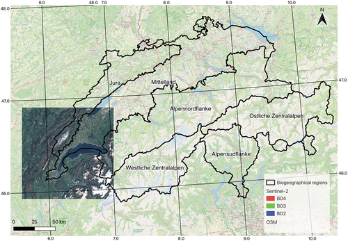
These areas cover a range of landscapes and ecological attributes distinguished by diverse climatic, geological, and vegetative characteristics. Segmented by altitude, they can be categorized into three primary zones: the Alps (North, Central, South), marked by high elevations covering 60% of the country’s total surface area, while the Plateau (30%) and the Jura (10%) feature lower elevations. Switzerland’s climate is significantly influenced by its proximity to the Alps and the Atlantic Ocean. Across the country, the climate is moderately continental on the plateau, alpine in mountainous regions, and relatively temperate in the Southern Alps. Switzerland experiences four distinct seasons, each exhibiting varying temperature and precipitation patterns aligned with these diverse climatic conditions (NCCS, 2018).

3. Methodology & implementation

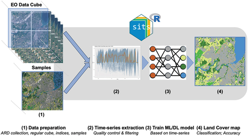
The applied time-first approach for land cover mapping follows the general workflow summarized in Figure 2. Collections of Big EO data are organized as data cubes on which spatial location is associated with a time-series. Samples with known labels train a Machine Learning (ML) or a Deep Learning (DL) algorithm that will classify unlabeled time-series of a data cube (Camara et al., 2016; Simoes et al., 2021). Hereafter, we used a time-series of Sentinel-2 data covering the whole 2018 year together with samples from the official Land Use Statistics (Arealstatistik) over the greater Geneva area (Switzerland). The workflow has been implemented in R (4.3.1) using Rstudio (2023.06.1 + 524) and the SITS package (version 1.4.1).

Figure 2. General workflow for the land cover map production using with the SITS package in R.

3.1. SITS – Satellite Image Time Series Analysis on Earth Observation Data Cubes

SITS is an R package (https://cran.r-project.org/web/packages/sits/index.html) for land use and land cover (LUC) classification from Big EO data made freely and openly available from Data Cubes (e.g. Brazil, Switzerland, Digital Earth Africa) (Ferreira et al., 2020; Giuliani et al., 2017; Sudmanns et al., 2022) or large image collections (e.g. Amazon Web Services, Microsoft Planetary Computer) (Gomes et al., 2020). It is a wall-to-wall integrated solution, through an Application Programming Interface (API) that provides effective tools for all steps of LUC classification workflow: sampling selection, time series clustering, machine learning model training and validation, classification, and maps post-processing (https://e-sensing.github.io/sitsbook/). Users usually follow a four-steps workflow that corresponds to dedicated functions of the SITS API (Table 1):

1. Data preparation

   • Select an analysis-ready data image collection: [sits_cube()]

   • Build a regular data cube using the selected image collection: [sits_regularize()]

   • Compute new bands and indices: [sits_apply()]

2. Time-series extraction

   • Extract time-series from samples and data cube that will be used as training data: [sits_get_data()]

   • Perform quality control, and filtering of noisy samples in the time series: [sits_reduce_imbalance(); sits_som_map(); sits_kfold_validate()]

3. ML/DL model training

   • Train a ML/DL model using the time series samples: [sits_train()]

4. Land cover map production

   • Classify the data cube using the model to get class probabilities for each pixel: [sits_classify()]

   • Post-process the probability cube to remove outliers: [sits_smooth()]

   • Produce a labeled map from the post-processed probability cube: [sits_label_classify()]

   • Evaluate the accuracy of the classification using best practices: [sits_accuracy()]

Table 1. SITS API main functions and their respective inputs and outputs (adapted from SITS book).

Step	API_function	Inputs	Output
1	sits_cube()	ARD image collection	Irregular data cube
	sits_regularize()	Irregular data cube	Regular data cube
	sits_apply()	Regular data cube	Regular data cube with new bands and indices
2	sits_get_data()	Data cube and sample locations	Time series
	sits_reduce_imabalance()	Time series samples	Balanced time-series
	sits_som_map()	Balanced time-series	Clean balanced time-series
	sits_kfold_validate()	Clean balanced time-series	Confusion matrix + F1 scores
3	sits_train()	Time series and ML method	ML classification model
4	sits_classify()	ML classification model and regular data cube	Probability cube
	sits_smooth()	Probability cube	Post-processed probability cube
	sits_label_classification()	Post-processed probability cube	Classified map
	sits_accuracy()	Classified map and validation samples	Accuracy assessment

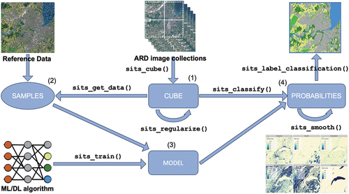
Figure 3 depicts the main functions of the SITS API and their respective interactions and links with the different steps from the data preparation to the production of the final LUC map.

Figure 3. Main functions of the SITS API and their respective interactions in the processing chain.

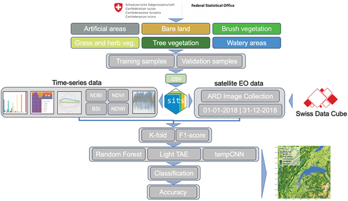
Following the general approach using SITS, the implemented workflow uses the Swiss Data Cube to access satellite Analysis Ready Data (ARD) and the Arealstatistik for the Reference data (Figure 4). The classification schema is the NOLC04 (https://www.bfs.admin.ch/bfs/de/home/statistiken/raum-umwelt/nomenklaturen/arealstatistik/nolc2004.html) for the 6 Principal Domains; the spectral time-series are complemented with spectral indices for enhancing the detection of vegetation (Normalized Difference Vegetation Index – NDVI), water (Normalized Difference Water Index – NDWI), built-up (Normalized Difference Built-up Index – NDBI) and bare areas (Bare Soil Index); finally one ML algorithm (Random Forest) and two DL algorithms (Light TAE, tempsCNN) have been tested. Each major steps of the workflow are further detailed in the following sub-sections.

Figure 4. General implementation of the workflow in SITS. Satellite Analysis Ready Data are provided by the Swiss Data Cube (https://www.swissdatacube.ch); samples are gathered from the Arealstatistik dataset provided by the Federal Statistical Office.

3.2. Data preparation

The first step consists in gathering (1) reference data (also referred as samples) and (2) multi-spectral data time-series provided by a Data Cube. They will then be used to extract time-series and for which label (i.e. classes) are known.

3.2.1. Satellite data

In SITS, satellite data are obtained from different cloud-based services that provides access to data are ready for analysis. According to the Committee on Earth Observation Satellites (CEOS), Analysis Ready Data (ARD) have been “processed to a minimum set of requirements and organized into a form that allows immediate analysis” (Dwyer et al., 2018; Lewis et al., 2018). In this work, satellite imagery is provided by the Swiss Data Cube (SDC – https://www.swissdatacube.ch). The SDC, operated jointly by the University of Geneva, the United Nations Environment Programme/GRID-Geneva, the University of Zurich, and the Federal Institute for Forest, Snow, and Landscape Research, aims to establish a consistent, dependable, and operational service. Leveraging satellite Earth Observations (EO), the SDC provides decision-ready products to empower policymakers, scientists, the private sector, and civil society to address social, environmental, and economic changes on a national scale. It fosters an ecosystem for innovation across sectors (Dhu et al., 2019; Giuliani et al., 2020; Obuchowicz et al., 2023; Poussin et al., 2021). This cloud-based analytical platform grants users’ access to over 40 years of optical (e.g. Sentinel-2; Landsat-5, -7, -8, -9) and radar (e.g. Sentinel-1) imagery (Chatenoux et al., 2021; Truckenbrodt et al., 2019). The archive is regularly updated, comprising approximately 80,000 scenes totalling 30 TB and encompassing over 3,000 billion observations/pixels.

Data have been downloaded using the sits_cube() function and the SpatioTemporal Asset Catalog (STAC) interface of the SDC (https://explorer.swissdatacube.org/stac/collections) allowing to access all available Sentinel-2 images (with 12 bands) for the year 2018 (to match with the latest data of the Arealstatistik) corresponding to a total amount of 113 scenes covering the tile 31TGM that corresponds to the area of interest (Drusch et al., 2012). A key requirement for effective classification using ML/DL techniques is that input data should be consistent in space, time, and bands. There should be no gaps or missing values, and therefore dimensionality of data used to train a model has to be the same of the data to be classified (Appel & Pebesma, 2019). The sits_regularize() function helps ensuring that all cells of the data cube have the same spatiotemporal extent, the same resolution, the same temporal interval and each cell contains a valid set of measures. Finally, to complement the spectral bands of the regular cube and enhance the separability of LUC classes, it is recommended to add different spectral indices, that is well-established practice in remote sensing (Chaves et al., 2023). Using the sits_apply() function we computed for each scene, the Normalized Difference Vegetation Index (NDVI), the Normalized Difference Water Index (NDWI), the Normalized Different Built-up Index (NDBI), and the Bare Soil Index (BSI) (Montero et al., 2023). This will help to discriminate between vegetation, water, built, and bare structures. At the end of this process, a regular data cube with the 12 spectral bands and 4 indices is available.

3.2.2. Reference data

The official source of LUC data maintained and made freely available by the Federal Statistical Office (FSO) (https://www.bfs.admin.ch/bfs/en/home/services/geostat/swiss-federal-statistics-geodata/land-use-cover-suitability/swiss-land-use-statistics.assetdetail.25885691.html) has been used as reference data. The Arealstatistik dataset is produced by visual interpretation of aerial photography and my assigning Land Cover (LC) and Land Use (LU) categories to 4 million sample points over the country from a regularly space 100 m grid (Beyeler et al., 2021; Swiss Federal Statistical Office, 2001). Gridded LC maps can then be obtained by rasterizing the sampling points of the Arealstatistik dataset and assigning a pixel value based on the lower-left corner point (Federal Statistical Office - FSO, 2007) (Figure 5).

Figure 5. Aerial view over an area in Geneva (left); the sample points from the arealstatistik with the different classes of the NOLC04 Principal Domains (middle); and the translation in gridded land cover map (right).

In this study, we used as reference data the samples from the latest survey period (2013–2018). A subset of reference data covering the study area includes around 410,000 features that are separated in training and validation data using the commonly agreed 70/30% separation threshold (Shetty et al., 2021) corresponding approximately to 287,000 samples for training and 123,000 for validation. For the LC classification, the NOLC04 classification schema has been used. It considers 27 “Basic Categories” but for better statistical reliability, especially for the use on a small scale, these categories are aggregated into 6 “Principal Domains” (Table 2). Consequently, it has been decided to consider the Principal Domains to test the time-first approach.

Table 2. Categories following the land cover NOLC04 classification separated in principal domains and basic categories.

Principal Domains	Basic Categories
10 – Artificial areas	15 – Lawns
	16 – Trees in artificial areas
20 – Grass and herb vegetation	21 – Gras and herb vegetation
30 – Brush vegetation	31 – Shrubs
	32 – Brush meadows
	33 – Short-stem fruit trees
	34 – Vines
	35 – Permanent garden plants and brush crops
40 – Tree vegetation	41 – Closed forest
	42 – Forest edges
	43 – Forest strips
	44 – Open forest
	45 – Brush forest
	46 – Linear woods
	47 – Cluster of trees
50 – Bare land	51 – Solid rock
	52 – Granular soil
	53 – Rocky areas
60 – Watery areas	61– Water
	62 – Glacier, perpetual snow
	63 – Wetlands
	64 – Reedy marshes

3.3. Time-series extraction and training samples improvements

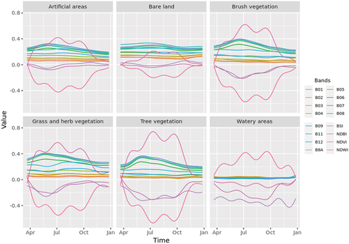
The second step of the workflow is aiming to extract time-series for the training samples from the regular data cube using the function sits_get_data(). At the end of the process, users obtain for each point of the reference data, time-series from the 12 spectral bands and 4 indices. This requires to deal with large time-series, and therefore to adequately capture the temporal variability of each class, patterns could be extracted with SITS using the time-weighted dynamic time warping for satellite image time series approach (dtwSat) (Maus et al., 2019). Using a Generalized Additive Model (GAM), single time-series can be approximated and giving insights over the time-series behavior and the separability of each class (Figure 6).

Figure 6. Patterns of the time-series for the six classes extracted using SITS. Each of six Principal Domains show different patterns that indicate potential good separability between the classes.

Based on these time-series, then a critical action requires selecting good training samples to achieve accurate results (Bratic et al., 2023; Hermosilla et al., 2022). It has been showed that number and quality of training samples are fundamental factors to obtain high-accuracy results (Maxwell et al., 2018). Ideally, large and accurate training datasets are preferable, independently of the algorithm used, while noisy training samples can significantly reduce classification performance (Frenay & Verleysen, 2014). Consequently, pre-processing methods to enhance the quality of training samples by removing those that are incorrectly labelled and present low discriminatory power, is an essential task before training any ML/DL model.

In SITS, this quality control and filtering of noisy samples can be done through three processes: (1) cross-validation of training samples; (2) sample quality control; and (3) reducing sample imbalance. The first step allows to estimate the inherent prediction error of a model using the k-fold validation method available in the sits_kfold_validate()function (Loew et al., 2017; Mayr et al., 2019; Olofsson et al., 2013). An important point to consider is that cross-validation is not an accuracy measure of the overall map, since it is difficult to collect random stratified training samples that cover all variations in land classes associated within a given ecosystem (Wadoux et al., 2021). Cross-validation only measures how good a model fits the training samples. Indeed, training samples are subject to various sources of errors (class representativity, noisy samples, labelling errors) and consequently cross-validation should not be considered as an accuracy estimation of the entire dataset but instead represents a measure of model performance. Quality control is achieved through a clustering technique based on Self-Organizing Maps (SOM), with the sits_som_map() function, that is a dimensionality reduction technique in which high-dimensional data is mapped into a two-dimensional map, while preserving the topological relations between data patterns. This approach has demonstrated to be an effective method to filter noisy samples and evaluate which spectral bands and indices are most suitable to enhance the separability of LUC classes (Santos et al., 2020). SOM map is composed of units, called neurons, that have weight factors with the same dimension as the training samples. The algorithm is trained by competitive learning and computes the distance of each sample to all neurons and identifies the nearest neuron to the inputs data, also referred to the best matching unit. The resulting output is a set of clusters, providing information on intra- and inter-class variability, allowing to detect noisy samples, and measuring confusion between labels. Good quality samples are assumed to have homogenous neurons (high frequency for one label), while heterogenous neurons (two or more labels with significant frequencies) contains probably noisy samples that could be removed with the sits_som_clean_samples() function. This function identifies which samples are noisy, clean, and those that needs to be further inspected by the user. Finally, the last process concerns the reduction of imbalance of training samples, since usually the distribution of EO-based training samples associated with each label is uneven. It has been recognized that such property can negatively influence classification accuracy (Johnson & Khoshgoftaar, 2019). The function sits_reduce_imbalance() implements the Synthetic Minority Over-sampling TEchnique (SMOTE) method to increase the number of samples of least frequent labels, and reduces the number of samples of most frequent labels (Chawla et al., 2002; Elreedy & Atiya, 2019).

At the end of this process, it ensures that training samples are of sufficient quality enhancing discrimination of classes, with less confusion to train ML/DL models efficiently and effectively. Figure 7 shows the confusion between the clusters produced by a SOM analysis for the training samples before and after undergoing the pre-processing (e.g. SOM cleaning and classes imbalance reduction) of training samples. This shows a significant improvement, with less confusion between the classes and an improved representativity of each class (Table 3). Nevertheless, it should be noted that the process led to an important reduction of the number of training samples. It is mostly caused by the imbalance reduction. The two most frequent labels (Grass and herb vegetation; Tree vegetation) represent 72% of all samples, while the two least frequent labels (Bare land; Brush vegetation) account for 0.5%. Such behavior is inadequate as ML algorithms are usually more accurate for classes with higher representativeness. Therefore, reducing imbalance can significantly enhance the classification accuracy, despite the significant reduction of training samples number. Sample size also affects the final LUC map accuracy, and a possible improvement is to use a higher number of synthetic samples generated by the SMOTE method (Elreedy & Atiya, 2019).

Figure 7. Confusion by cluster between the six different classes before (left) and after (right) pre-processing of the training samples.

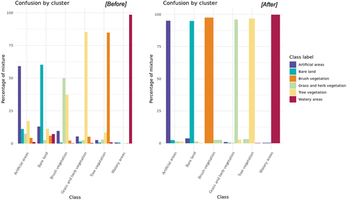
Table 3. Proportion of samples before and after the pre-processing of the training samples.

	Before pre-processing		After pre-processing
Label	Count	Proportion	Count	Proportion
Artificial areas	28884	0.10114862	1600	0.19314341
Bare land	7621	0.02668791	1150	0.13882183
Brush vegetation	9109	0.03189873	806	0.09729599
Grass and herb vegetation	120237	0.42105687	1600	0.19314341
Tree vegetation	86169	0.30175445	1600	0.19314341
Watery areas	33540	0.11745342	1528	0.18445196

3.4. ML/DL models training

SITS implements different machine learning methods that can be considered as supervised classification used to train an algorithm to predict which class an input data belongs to. It classifies individual time-series using the time-first approach mentioned in the introduction using two sets of methods: (1) Machine Learning (ML) techniques that do not explicitly consider the temporal structure of a given time-series such as Random Forest (RF) or Support Vector Machin (SVM) (Gislason et al., 2006; Maxwell et al., 2018; Thanh Noi & Kappas, 2017); and (2) Deep Learning (DL) methods where temporal relations between observed values of a time-series are considered like the Temporal Convolution Neural Network (tempCNN) or Lightweight Temporal Self-Attention Encoder (LTAE) (Cheng et al., 2023; Fawaz et al., 2018; Pelletier et al., 2019; Sainte Fare Garnot et al., 2020).

In the present work, it has been decided to compare the most frequently used ML method (i.e. Random Forest) to two emerging DL methods (i.e. tempCNN and LTAE) that are gaining interest in the community (Papoutsis et al., 2023). All these methods are available using the sits_train() function that provides a standardized interface to train various ML/DL algorithms. SITS provides a set of reasonable default values that help novice users to train their models, while expert users can fine-tune the model parameters using the sits_tuning() function.

3.5. Land cover map classification and accuracy measurements

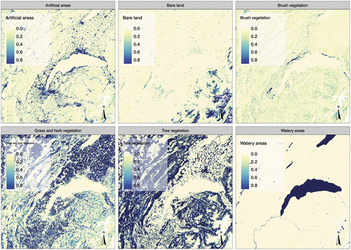
The final step of the workflow consists in using the trained model to classify the data cube with the time-series with the sits_classify() function. The result of this process is a data cube with a set of probability layers, one for each class, that determines how likely a give pixel belongs to a certain class (Figure 8).

Figure 8. Smoothed probabilities obtained for the tempCNN model and each land cover classes according to the NOLC04 nomenclature.

To reduce outliers, often visible as small patches surrounded by a different class, or misclassified pixels, pixels which show large data variability, SITS implements post-processing smoothing techniques, with the sits_smooth() function that takes into account the spatial neighboring and context. This reduces the salt-and-pepper as well as border effects enhancing the quality of classification and interpretability of the resulting map. Based on these smoothed probabilities, then users can apply the sits_label_classification() function to produce the LUC map by assigning the label with the highest probability to a given pixel.

Finally, to quantify the quality of the resulting LUC map, accuracy and uncertainty of the classified images should be evaluated. This is an important aspect to consider ensuring that results are reliable and potentially valid to support decision-making. SITS implements the sits_accuracy() function that follows the best practices proposed by Olofsson et al. (2013 and 2014) using an area-weighted technique to take into account that land classes are not evenly distributed in space. This process uses the validation samples that were produced in the first step of the workflow. Uncertainty is measuring the confidence level of the resulting map. There are several potential causes of uncertainty such as classification errors, ambiguity of the classification schema, variability of the landscape, or limitations of the data (Camara et al., 2016). In SITS, the sits_uncertainty() function allows estimating the entropy (i.e. the difference between all predictions expressed) of the produced land cover map. It uses the probabilities produced by the classifier to compute the amount of variability in the probabilities related to a pixel. The higher the variability, the higher the entropy. Such estimates are important to communicate, helping to identify areas that requires further investigation and/or samples collection. In complement, confusion and error matrices can be used to evaluate the uncertainty of classification results.

4. Results

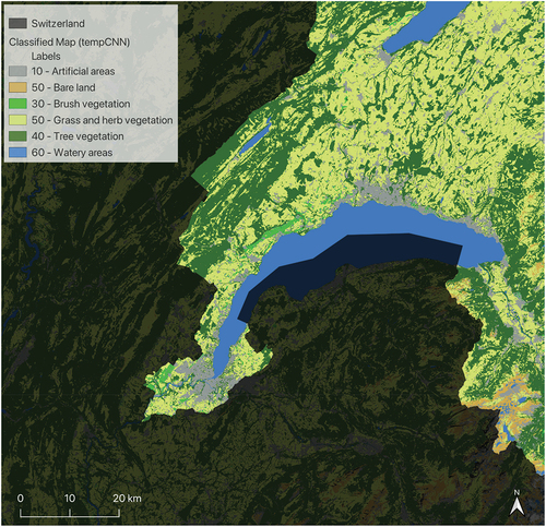
One of the main objectives of the present work was to test a time-first approach with different ML/DL algorithms to classify Sentinel-2 data according to the national NOLC04 nomenclature of the six Principal Domains. The final output map (Figure 9) has been produced using a tuned tempCNN model which resulted being the optimal choice to achieve high classification accuracy results. Visually, the landscape is largely dominated by “Grass & Herb vegetation”, “Watery areas” and “Artificial areas”.

Figure 9. Final output of the classification obtained with the tempCNN model.

Results from the cross-validation on the balanced training samples showed that both DL models (i.e., LTAE and tempCNN) and ML model (i.e. RF) have almost similar performances and do not allow to identify an algorithm that will significantly outperform the others (Table 4). Values of accuracy (i.e. number of times a model is able to correctly identify the class across the training dataset); confidence interval (i.e. interval which is expected to typically contain the parameter being estimated); Kappa coefficient (i.e. comparison between observed and expected accuracies (random chance)) and F1 score (i.e. average of precision and recall, accounting for the type of errors – false positive and false negative) for the three models are very close to each other with the RF model that has the higher values.

Table 4. Cross-validation showing accuracy, 95% Confidence Interval (CI), Kappa values, and F1-scores for the three tested methods: Random Forest (RF), lightweight temporal self-attention encoder (LTAE), and temporal convolutional neural network (tempCNN).

		RF	LTAE	tempCNN
Accuracy		0.9849	0.9703	0.9794
95% CI		(0.982, 0.9874)	(0.9664, 0.9739)	(0.9761, 0.9823)
Kappa		0.9817	0.964	0.975
F1-scores	Artificial areas	0.9812	0.9659	0.9697
	Grass and herb vegetation	0.9758	0.9528	0.9723
	Tree vegetation	0.9853	0.9798	0.9828
	Watery areas	0.9980	0.9951	0.9980
	Brush vegetation	0.9894	0.9655	0.9926
	Bare land	0.9817	0.9575	0.9634

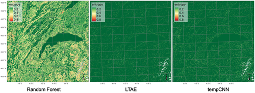
However, when looking at the uncertainty maps, then it appears that DL models have significantly less uncertainty than RF-based classification (Figure 10).

Figure 10. Uncertainty of RF, LTAE, tempCNN models estimated through entropy estimation.

In terms of classification accuracy, Table 5 summarizes the overall, as well as the users and producers’ accuracies for three models. Overall accuracy represents the proportion of correctly classified samples from the reference data. Producers’ accuracy (i.e. omission errors) represents how well reference pixels of the ground cover type are classified, whereas Users’ accuracy (i.e. commission errors) represents the probability that a pixel classified into a given category represents that category on the ground.

Table 5. Overall, users (UA) and producers (PA) accuracy for three models produced with a time-first approach and a comparison with the space-first approach.

	Space-first		Time-first
	RF		RF		LTAE		LTAE (tuned)		tempCNN		tempCNN (tuned)
Overall	0.82		0.85		0.83		0.86		0.86		0.90
	UA	PA	UA	PA	UA	PA	UA	PA	UA	PA	UA	PA
Artificial areas	0.65	0.61	0.67	0.63	0.75	0.54	0.69	0.65	0.69	0.65	0.75	0.67
Bare land	0.79	0.42	0.65	0.38	0.57	0.40	0.64	0.41	0.64	0.41	0.72	0.49
Brush vegetation	0.59	0.11	0.68	0.11	0.38	0.23	0.68	0.15	0.68	0.15	0.71	0.19
Grass and herb vegetation	0.82	0.82	0.87	0.87	0.86	0.83	0.88	0.89	0.88	0.89	0.91	0.89
Tree vegetation	0.83	0.85	0.85	0.95	0.82	0.95	0.86	0.95	0.86	0.95	0.87	0.97
Watery areas	0.96	0.90	0.99	0.90	0.99	0.89	0.99	0.90	0.99	0.90	0.99	0.90

Results indicate that besides the fact that Random Forest model is giving reasonable classification accuracies both overall and by class, the best results in undeniably the tempCNN model with tuned hyperparameters. Indeed, this model is producing high classification accuracy values with less uncertainties in the model and therefore it appears to be the best choice. Nevertheless, the “brush vegetation” class, has the lowest accuracy with all tested methods. This is principally caused by the varieties of vegetation density and types that could produce dissimilarities in the same LUC class. Indeed, if we look at Table 2, the “brush vegetation” class is composed of five different types of vegetation that are quite diverse and that could explain this low accuracy. Moreover, low values could occur in areas where different features were either mixed up or in proximity. Consequently, testing the time-first approach on “Basic categories (i.e. 27 classes of LC) could help in better characterizing and discriminating the different “brush vegetation” classes and possibly enhance the accuracy of this class.

To highlight the benefit of a time-first approach, results have been compared with the work done by Thomas and Giuliani (2023) who used a space-first approach. They used the same satellite data (i.e. Sentinel-2 for 2018, tile 31TGM) over the same area. However, they produced a yearly cloud-free composite using the a geometric median (geomedian) algorithm which effectively handle a temporal stack of noisy observations for a single high-quality pixel composite with reduced spatial noise (Roberts et al., 2017). In contrast to a standard median, a geomedian maintains the relationship between spectral bands. Then she trained a Random Forest classifier using the same reference data (Arealstatistik) obtaining a best overall accuracy of 0.82 and class accuracies are generally lower (e.g. ranging from 2% to 10%) than the values obtained from our time-first RF model. The larger gains in term of accuracies between the two approaches are for vegetation classes that show a larger variability across the year than less dynamic classes such as artificial areas. This reveals that the time-first approach is giving improved results compared to a space-first approach both from overall and per class accuracies.

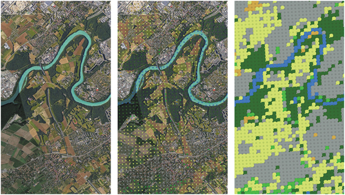
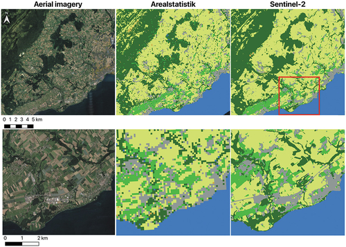
Finally, visually comparing the results with the reference dataset (i.e. Arealstatistik), it shows, the high-level of confidence of the produced map, together with an increased spatial resolution that removes the “salt and pepper” effect of the Arealstatistik and consequently enhancing the capacity to capture more subtle elements of the landscape (Figure 11).

Figure 11. Visual comparison of an aerial image (left) with Arealstatistik (middle) and the classified Sentinel-2 data with the tuned tempCNN model (right). The top view shows a larger area than the bottom view that corresponds to a zoom in the red square. Legend is the same as Figure 9.

An important argument from the Federal Statistical Office about the use of the Arealstatistik is that it significantly describes the different classes, meaning that the proportions between the different classes are statistically representative and therefore it is critical to compare with the proportion obtained with the classified map. Number of pixels, the surface and the proportion of the resulting map have been computed in QGIS using the classification report tool of the Semi-Automatic Classification plugin (Congedo, 2021). Despite some small differences, the proportions are nearly similar indicating that the proposed method is spatially consistent with the official LUC data for Switzerland (Table 6).

Table 6. Comparison of the proportions by class between the Arealstatistik and the classified Sentinel-2 data with the tuned tempCNN model.

	Arealstatistik			Sentinel-2
	Number (points)	Surface (km^2)	Proportion (%)	Number (pixels)	Surface (km^2)	Proportion (%)
Artificial areas	41588	415.88	10.14	4065402	406.54	9.91
Bare land	48250	482.5	11.77	4549149	454.92	11.09
Brush vegetation	12374	123.74	3.02	956667	95.67	2.33
Grass and herb vegetation	171829	1718.29	41.90	17766483	1776.65	43.32
Tree vegetation	13078	130.78	3.19	1081687	108.17	2.64
Watery areas	122992	1229.92	29.99	12589829	1258.98	30.70
Total	410111	4101.11	100.00	41009217	4100.92	100.00

5. Discussion

The obtained results show that the proposed approach can contribute to tackle the need of accurate, consistent, and increased spatial resolution of LUC information at national scale. In particular, the addition of temporal features, considering the intra-annual variability of classes, brought significant gains in term of accuracy and separability of the classes compared to single date results (i.e. space-first). Here, the incorporation of time-series of both spectral bands and indices over a full year improved the classification performance. Results also indicate that Deep Learning methods appear to outperform more traditional and widely used Machine Learning methods such as Random Forest. Notably, DL methods have less uncertainty than ML, which is an essential aspect to consider for effective change detection. Additionally, good training samples (i.e. clean, and balanced) and hyperparameters tunning are two factors to carefully consider for achieving satisfactory classification performance. Overall, the tempCNN algorithm with tuned hyperparameters has been identified as the most convenient method to produce accurate and robust predictions using the Arealstatistik as training dataset.

The final land cover map is much more detailed compared to the official national LUC product, having a spatial resolution 10 times higher, allowing to capture elements of the landscape that are currently not visible in the Arealstatistik. Moreover, it removes the “salt&pepper” effect and therefore LUC change can be potentially easier to identify and assess (Giuliani et al., 2022; Thomas & Giuliani, 2023). The generated product as a high accuracy, both overall and by class, and an improved georeferencing making spatial analysis of change easier and more consistent. Ultimately, the observation that the produced map largely maintains statistical significance, by preserving the proportions of the original Arealstatistik classes, suggests that the proposed method can likely be employed for effective monitoring of LUC change in Switzerland.

However, to achieve that objective, some limitations should be further properly addressed. The most important limitation to tackle is to increase the temporal resolution of the LUC information. Indeed, with a survey available every 6 years allows capturing only slow onset changes (Thomas & Giuliani, 2023). Nevertheless, for efficient and effective environmental monitoring, rapid onset LUC change should be also identified. Therefore, having annual land cover products would facilitate the identification and understanding of LUC processes, pressures and drivers and their influence on climate, biodiversity, and ecosystems (Bontemps et al., 2013; Kennedy Robert et al., 2014; Teixeira et al., 2014). Currently, with the current proposed approach, it is only possible to use training samples of the same acquisition period of the satellite data. Transfer Learning methods could help to tackle this issue by allowing the reuse of models trained on specific years to classify subsequent or preceding years, eliminating the need for new training samples every year (Alem & Kumar, 2022). Another limitation concerns the fact that currently, in the pre-processing of the training samples, spatial autocorrelation is not taken into account and consequently can influence the quality of the training samples potentially causing overfitting in the tested models (Phan et al., 2022). To reduce that effect, point samples could be selected based on minimum distance criteria (e.g. 1 km), ensuring that training samples are covering the entire study area.

The proposed approach shows the benefits of a synergetic use of statistical sampling survey and satellite data for LUC mapping. The generated product shows a lot of potential but is not aiming at replacing the official Arealstatistik but instead it could significantly complement it. An inspiring example is the Portuguese Land Cover Monitoring System (Costa et al., 2023) that had similar concerns with the official LUC information being produced by photo-interpretation on a 3–5 years basis. Despite the emergence of improved LUC products provided by the Copernicus Land Monitoring Service their applicability at national scale are still limited (Verde et al., 2020). Therefore, Portugal decided to explore approaches to complement the existing LUC information with space-based products tacking into account requirements of national end-users. As of today, the official LUC map, more focused on land use, is complemented with an annual land cover map generated using classification of Sentinel-2 and ML-based algorithms. Such complementary approaches can pave the way to implement continuous land change monitoring capabilities such as the Land Change Monitoring, Assessment, and Projection (LCMAP) approach (Brown et al., 2019).

This work represents the initial step towards the ambitious objective to contribute to a consistent, continuous, and accurate land monitoring system nationwide. Nevertheless, there are many possibilities to improve these first results. Hereafter, we list some ideas of improvements that we will further tested in the next iteration of our research work:

1. Test the proposed approach on the 27 Basic Categories: indeed, our work is currently restricted to the 6 Principal Domains that described the main land cover classes of the Swiss landscape. However, it is essential to also produce a map of the 27 official land categories.

2. Add additional predictors: related to the previous point, with many different land cover classes, it will require adding predictors to further enhance the discriminatory power of the proposed approach. We suggest to add contextual data like Digital Elevation Model (DEM) (Sang et al., 2021) and other spectral indices like to Normalized Difference Snow Index (NDSI) (Poussin et al., 2023) and the Anthocyanin Reflectance Index (ARI) (Bayle et al., 2019) that could result in better identifying snow and grassland/shrublands and discriminate classes based on altitudinal attributes.

3. Explore the use of PPI instead of NDVI: due to the fact that our work is based on time-series and de facto it includes some phenological metrics (having time-series of NDVI), some studies have shown that the Plant Phenology Index (PPI) has improved performance over NDVI in retrieval of phenological metrics (Karkauskaite et al., 2017; Jin & Eklundh, 2014). Therefore, we can make the reasonable assumption that using PPI instead of NDVI could further improve the accuracy and discrimination of vegetation classes.

4. Improving the quality of training samples: comparative analysis of different machine learning methods show that the quality of training samples has a large impact on LUC classification accuracy (Pelletier et al., 2017; Maxwell et al., 2018). Training samples must properly describe the diversity and representativity of LUC classes that are supposed to be identified by the classifier. The quality of LUC samples depends on (1) the accuracy of the samples regarding the classes they represent; (2) their coverage of the whole range of the classes’ spectral variety, and (3) their adherence to an appropriate sampling design. SITS already implement different filtering and clustering techniques that could improve the initial implementation as well as sampling strategies (e.g. random stratified with minimum distance attribute) could also further enhance the quality of training samples.

5. Reducing uncertainty: one of the main challenges in image classification is to adequately describe the diversity of landscape. Consequently, this leads to approximation in the description of the landscape and potential errors and related uncertainty. To reduce these errors and uncertainty and improve accuracy, there are several possibilities to be used such as Active Learning, an iterative process of sample selection, labelling, and model retraining (Safonova et al., 2023; Chen et al., 2023; Tuia et al., 2023); Ensemble modelling: combining predictions from multiple models to produce more accurate and robust predictions (Chai & Li, 2023; Du et al., 2023; Song et al., 2023; Xu et al., 2023); and Mixture model: to decipher the contributions of mixture of spectral responses of different land cover types inside a pixel and obtain the proportion of a given class inside a mixed pixel (Quintano et al., 2012; Halbgewachs et al., 2022; Shimabukuro & Ponzoni, 2019).

6. Object-based time-series analysis: Object-Based Image Analysis (OBIA) is increasingly used to extract meaningful information it in medium resolution images like Sentinel-2. The group of pixels with similar time-series responses (also known as super-pixels) can be used to spatially portioning the image and assigned it to a single class. Such process, when applicable can reduce processing time and produce LUC maps with enhance spatial consistency (Chaves et al., 2023). In such an approach, the large-scale topographic landscape model (TLM – https://www.swisstopo.admin.ch/en/geodata/landscape/tlm3d.html) of Switzerland could be used as a reference dataset for segmentation and model training.

7. Land Use mapping: current efforts have been focused on land cover but obviously exploring a time-first approach for land use mapping with the NOLU04 (4/10/46 categories) nomenclature and classification schema is important to precisely map, not only the physical aspect of the Swiss landscape but also how they are used.

8. Exploring the use of Landsat: in the present work Sentinel-2 data were used for their increased spatial and temporal resolution. However, Landsat is the longest EO data archive and it would be valuable to leverage the benefits of the presented approach with long time-series of observations done by the Landsat programme (Loveland et al., 2022; Wulder et al., 2022; Zhang et al., 2022).

Finally, it shouldn’t be forget that the use of satellite EO data for LUC classification requires dealing with various compromises arising from different constraints: (1) measurements from a given sensor (or combination of sensors) are restricted by spectral, temporal, and spatial resolution, therefore defining the boundary conditions of land classes separability; (2) the objective of generating LUC maps that adequately conform to abstract descriptions of the Earth’s ecosystems as defined in typologies like FAO Land Cover Classification System (LCCS) (DiGregorio, 2016) or EAGLE (Arnold et al., 2013); (3) the need for effectively describe land change (e.g. anthropization); and (4) the prerequisite to achieve high accuracy when using EO data for compliance and public policy (e.g. deforestation). As matter of fact, these constraints inherently conflict with each other, making it unfeasible to classify EO data in a manner that equally satisfies all users at the same time. Current LUC products (e.g. ESA 10 m World Cover) fall short in differentiating between natural savannas and anthropic grasslands, a critical distinction for monitoring biodiversity loss. Instead of starting with what is measurable with satellite observations, numerous data producers adopt a data-independent taxonomy that does not align with the data. Consequently, taking a case-by-case data-driven approach will certainly help to get the most from the available technologies for improving predictability.

6. Conclusions

LUC data is considered as a fundamental information required to cope with the triple planetary crisis (i.e. climate change, biodiversity loss, pollution) as well as food security, sustainable management, and ecosystem services on which human well-being is critically dependent. Consequently, LUC change can be considered as a significant and visible indicator of human impact on the environment, serving as a crucial component supporting the formulation of efficient environmental and territorial policies. However, national products with high thematic accuracy supporting downstream applications (e.g. ecosystem, hydrology, atmosphere models) are still lacking and there is a critical need to have accurate, consistent, and high-resolution LUC products to effectively monitor landscape dynamics and better apprehend drivers, pressures, state, and impacts on land systems.

The proposed approach is a step towards this objective combining the thematic details of national photo-interpreted land use statistics with time-series of satellite EO data to produce an accurate and high spatial resolution land cover map. Our initial results indicate that the time-first approach appears to perform better than space-first approach, allowing capturing intra-annual variably of classes and consequently enhancing their identification. Among the tested methods, tempCNN (with tuned hyperparameters) is giving improved results compared to an attention-based model (LTAE) or the more traditional Random Forest. More generally, DL methods have shown lower uncertainties compared to the tested ML method, which is also an important aspect to consider for ultimately monitor land cover change. Overall, the produced Land Cover map has a high (overall and by class) accuracy, an improved spatial resolution allowing to detect more subtle details, while preserving the statistical significance (i.e. class proportion) of the official national dataset. Nevertheless, the next challenge to tackle is to increase the temporal resolution of the LUC information, to ultimately realize the objective to produce a yearly high-resolution land cover map of Switzerland. Such a product could potentially complement the official land use statistics, to take full advantage of a synergetic use of a statistical sampling survey and satellite data for LUC mapping.

Acknowledgements

The views expressed in the paper are those of the authors and do not necessarily reflect the views of the institutions they belong to.

Results of this publication are partly or fully relying on the Swiss Data Cube (http://www.swissdatacube.org), operated and maintained by UN Environment/GRID-Geneva, the University of Geneva, the University of Zurich and the Swiss Federal Institute for Forest, Snow and Landscape Research WSL.

We are grateful to the Data Science Competence Center (CCSD) and the Scientific Computing Support (SciCoS) of the University of Geneva who supported through the Data Science Impulse grant the “LC4SDG: Land Cover Data Science for the SDGs” project.

We would like to thank the LC4SDG team members for their valuable inputs at an early stage of the project: Prof. H. Dao, Prof. A. Lehmann, Prof. S. Marchand-Maillet, Dr. D. Rodila, B. Chatenoux, Dr. S. Biasse, as well as two students of the certificate of geomatics, Isabel Nicholson Thomas and Daniel Risse, who explored SITS.

Finally, we would like to thank Prof. Gilberto Camara, Prof. Karine Ferreira, Prof. Gilberto Queiroz and Mr. Felipe Sousa for their effective and appreciated support regarding SITS.

Disclosure statement

No potential conflict of interest was reported by the author(s).

Data availability statement

Sentinel-2 data that support the findings of this study are openly available at: https://doi.org/10.26037/yareta:zeg4u3pa5bcrfbph7mcsehorfm

Land Use Statistics, used as reference data are available at: https://www.bfs.admin.ch/bfs/de/home/statistiken/raum-umwelt/erhebungen/area.html

National Boundaries and Biogeographical regions can be obtained at: https://www.swisstopo.admin.ch/en/geodata/landscape/boundaries3d.html

Additional information

Funding

This research was funded by the Data Science Impulse grant of the University of Geneva.

Notes on contributors

Gregory Giuliani

Gregory Giuliani is the Head of the Digital Earth Unit and Swiss Data Cube Project Leader at GRID-Geneva of the United Nations Environment Programme (UNEP) and a Senior Lecturer at the University of Geneva’s Institute for Environmental Sciences. He is a geologist and environmental scientist who specializes in Remote Sensing, Geographical Information Systems (GIS) and Spatial Data Infrastructures (SDI). He also works at GRID-Geneva of the United Nations Environment Programme (UNEP) since 2001, where he was previously the focal point for Spatial Data Infrastructure (SDI) and is currently the Head of the Digital Earth Unit. Dr. Giuliani’s research focuses on Land Change Science and how Earth observations can be used to monitor and assess environmental changes and support sustainable development.

References

- Alem, A., & Kumar, S. (2022). Transfer learning models for land cover and land use classification in remote sensing image. Applied Artificial Intelligence, 36(1), 2014192. https://doi.org/10.1080/08839514.2021.2014192
- Appel, M., & Pebesma, E. (2019). On-demand processing of data cubes from satellite image collections with the gdalcubes library. Data, 4(3), 92. https://doi.org/10.3390/data4030092
- Arino, O., Gross, D., Ranera, F., Leroy, M., Bicheron, P., Brockman, C., Defourny, P., Vancutsem, C., Achard, F., Durieux, L., Bourg, L., Latham, J., DiGregorio, A., Witt, R., Herold, M., Sambale, J., Plummer, S., & Weber, J.-L. (2007). GlobCover: ESA service for global land cover from MERIS. 2007 IEEE International Geoscience and Remote Sensing Symposium, 2412–2415. https://doi.org/10.1109/IGARSS.2007.4423328
- Arnold, S., Kosztra, B., Banko, G., Smith, G., Hazeu, G., Bock, M., & Valcarcel Sanz, N. (2013). The EAGLE concept—A vision of a future European land monitoring framework. 3–6.
- Ban, Y. F., Gong, P., & Gini, C. (2015). Global land cover mapping using earth observation satellite data: Recent progresses and challenges. Isprs Journal of Photogrammetry and Remote Sensing, 103, 1–6. https://doi.org/10.1016/j.isprsjprs.2015.01.001
- Baraldi, A., Sapia, L. D., Tiede, D., Sudmanns, M., Augustin, H. L., & Lang, S. (2023a). Innovative Analysis Ready Data (ARD) product and process requirements, software system design, algorithms and implementation at the midstream as necessary-but-not-sufficient precondition of the downstream in a new notion of space economy 4.0 - part 1. Problem Background in Artificial General Intelligence (AGI) Big Earth Data, 7(3), 455–693. https://doi.org/10.1080/20964471.2021.2017549
- Baraldi, A., Sapia, L. D., Tiede, D., Sudmanns, M., Augustin, H., & Lang, S. (2023b). Innovative analysis ready data (ARD) product and process requirements, software system design, algorithms and implementation at the midstream as necessary-but-not-sufficient precondition of the downstream in a new notion of space economy 4.0 - part 2: Software developments. Big Earth Data, 7(3), 694–811. https://doi.org/10.1080/20964471.2021.2017582
- Bayle, A., Carlson, B. Z., Thierion, V., Isenmann, M., & Choler, P. (2019). Improved mapping of mountain shrublands using the sentinel-2 red-edge band. Remote Sensing, 11(23), 2807. Article 23. https://doi.org/10.3390/rs11232807
- Beyeler, N., Douard, R., Jeannet, A., Willi-Tobler, L., & Weibel, F. (2021). Land Use in Switzerland: Results of the Swiss Land Use Statistics 2018. Bundesamt für Statistik (BFS). https://dam-api.bfs.admin.ch/hub/api/dam/assets/19365054/master
- Bontemps, S., Defourny, P., Radoux, J., Van Bogaert, E., Lamarche, C., Achard, F., Mayaux, P., Boettcher, M., Brockmann, C., & Kirches, G. (2013). Consistent global land cover maps for climate modelling communities: Current achievements of the ESA’s land cover CCI, Proceedings of the conference ESA SP-722. 2-13, September 9-13 2013, Edinburgh, UK (p. 62).
- Boston, T., Van Dijk, A., & Thackway, R. (2023). Convolutional neural network shows greater spatial and temporal stability in multi-annual land cover mapping than pixel-based methods. Remote Sensing, 15(8), 2132. Article 8. https://doi.org/10.3390/rs15082132
- Bratic, G., Oxoli, D., & Brovelli, M. A. (2023). Map of land cover agreement: Ensambling existing datasets for large-scale training data provision. Remote Sensing, 15(15), 3774. https://doi.org/10.3390/rs15153774
- Brown, C. F., Brumby, S. P., Guzder-Williams, B., Birch, T., Hyde, S. B., Mazzariello, J., Czerwinski, W., Pasquarella, V. J., Haertel, R., Ilyushchenko, S., Schwehr, K., Weisse, M., Stolle, F., Hanson, C., Guinan, O., Moore, R., & Tait, A. M. Article 1. (2022). Dynamic world, near real-time global 10 m land use land cover mapping. Scientific Data, 9(1). https://doi.org/10.1038/s41597-022-01307-4.
- Brown, J. F., Tollerud, H. J., Barber, C. P., Zhou, Q., Dwyer, J. L., Vogelmann, J. E., Loveland, T. R., Woodcock, C. E., Stehman, S. V., Zhu, Z., Pengra, B. W., Smith, K., Horton, J. A., Xian, G., Auch, R. F., Sohl, T. L., Sayler, K. L., Gallant, A. L., Zelenak, D. … Rover, J. (2019). Lessons learned implementing an operational continuous United States national land change monitoring capability: The land change monitoring, assessment, and projection (LCMAP) approach. Remote Sensing of Environment, 238, 111356. https://doi.org/10.1016/j.rse.2019.111356
- Camara, G. (2020). On the semantics of big Earth observation data for land classification. Journal of Spatial Information Science, 20(20), 21–34. https://doi.org/10.5311/JOSIS.2020.20.645
- Camara, G., Queiroz, G., Vinhas, L., Ferreira, K., Cartaxo, R., Simoes, R., Llapa, E., Assis, L., & Sanchez, A. (2017). THE E-SENSING ARCHITECTURE FOR BIG EARTH OBSERVATION DATA ANALYSIS. Proceedings of the 2017 conference on Big Data from Space (BIDS’ 2017) (pp. 48–51). https://doi.org/10.2760/383579
- Camara, G., Simoes, R., Souza, F., Pelletier, C., Sanchez, A., Andrade, P. R., Ferreira, K., & Queiroz, G. (2016). Sits: Satellite Image Time Series Analysis on Earth Observation Data Cubes. Retrieved July 20, 2023, from https://e-sensing.github.io/sitsbook/
- Carlos, F. M., Gomes, V. C. F., Queiroz, G. R. D., Souza, F. C. D., Ferreira, K. R., & Santos, R. (2021). Integrating open data cube and brazil data cube platforms for land use and cover classifications. Revista Brasileira de Cartografia, 73(4), 1036–1047. Article 4. https://doi.org/10.14393/rbcv73n4-60387
- Chai, B., & Li, P. (2023). An ensemble method for monitoring land cover changes in urban areas using dense Landsat time series data. ISPRS Journal of Photogrammetry and Remote Sensing, 195, 29–42. https://doi.org/10.1016/j.isprsjprs.2022.11.002
- Chatenoux, B., Richard, J.-P., Small, D., Roeoesli, C., Wingate, V., Poussin, C., Rodila, D., Peduzzi, P., Steinmeier, C., Ginzler, C., Psomas, A., Schaepman, M., & Giuliani, G. (2021). The Swiss data cube: Analysis Ready data archive using earth observations of Switzerland. Scientific Data, 8(295). https://doi.org/10.1038/s41597-021-01076-6
- Chaves M, E. D., Picoli M, C. A., & Sanches, D. I. (2020). Recent applications of Landsat 8/OLI and Sentinel-2/MSI for land use and land cover mapping: A systematic review. Remote Sensing, 12(18), 3062. Article 18. https://doi.org/10.3390/rs12183062
- Chaves, M. E. D., Soares, A. R., Mataveli, G. A. V., Sánchez, A. H., & Sanches, I. D. (2023). A semi-automated workflow for LULC mapping via sentinel-2 data cubes and spectral indices. Automation, 4(1), 94–109. Article 1. https://doi.org/10.3390/automation4010007
- Chaves, M., Soares, A., Picoli, M., Simoes, R., Ipia, A., Lechler, S., & Sanches, I. (2023). GEOBIA and multitemporal segmentation for land use and land cover mapping: A case study in Mato Grosso, Brazil. Proceedings of the XX Brazilian Symposium on Remote Sensing - XX SBSR, Florianópolis (Vol. 20, p. 156009).
- Chawla, N. V., Bowyer, K. W., Hall, L. O., & Kegelmeyer, W. P. (2002). SMOTE: Synthetic minority over-sampling technique. Journal of Artificial Intelligence Research, 16, 321–357. https://doi.org/10.1613/jair.953
- Cheng, X., Sun, Y., Zhang, W., Wang, Y., Cao, X., & Wang, Y. (2023). Application of deep learning in multitemporal remote sensing image classification. Remote Sensing, 15(15), 3859. Article 15. https://doi.org/10.3390/rs15153859
- Chen, H., Yang, L., & Wu, Q. (2023). Enhancing land cover mapping and monitoring: An interactive and explainable machine learning approach using Google Earth Engine. Remote Sensing, 15(18), 4585. Article 18. https://doi.org/10.3390/rs15184585
- Comber, A., Fisher, P., & Wadsworth, R. (2005). What is land cover?. Environment & Planning. B, Planning & Design, 32(2), 199–209. https://doi.org/10.1068/b31135
- Congedo, L. (2021). Semi-automatic classification Plugin: A python tool for the download and processing of remote sensing images in QGIS. Journal of Open Source Software, 6(64), 3172. https://doi.org/10.21105/joss.03172
- Costa, H., Benevides, P., & Caetano, M. (2023). The Portuguese land cover monitoring system (SMOS): From research and development (R&D) to operations. REVISTA INTERNACIONAL MAPPING, 32(210), 44–51. https://doi.org/10.59192/mapping.387
- d’Andrimont, R., Verhegghen, A., Meroni, M., Lemoine, G., Strobl, P., Eiselt, B., Yordanov, M., Martinez-Sanchez, L., & van der Velde, M. (2021). LUCAS Copernicus 2018: Earth-observation-relevant in situ data on land cover and use throughout the European Union. Earth System Science Data, 13(3), 1119–1133. https://doi.org/10.5194/essd-13-1119-2021
- Delgado Hernández, J., & Valcárcel Sanz, N. (2022). National high-resolution land cover and land use information system. International Journal of Cartography, 8(1), 54–69. https://doi.org/10.1080/23729333.2021.1999051
- Dhu, T., Giuliani, G., Juarez, J., Kavadda, A., Killough, B., Merodio, P., Minchin, S., & Ramage, S. (2019). National Open Data Cubes and their contribution to country-level development policies and practices. Data, 4(4), 144. https://doi.org/10.3390/data4040144
- DiGregorio, A. (2016). Land cover classification system: Classification concepts. Software version 3.
- Drusch, M., Del Bello, U., Carlier, S., Colin, O., Fernandez, V., Gascon, F., Hoersch, B., Isola, C., Laberinti, P., Martimort, P., Meygret, A., Spoto, F., Sy, O., Marchese, F., & Bargellini, P. (2012). Sentinel-2: ESA’s Optical High-Resolution Mission for GMES operational services. Sentinel-2: ESA’s Optical High-Resolution Mission for GMES Operational Services Remote Sensing of Environment, 120, 25–36. https://doi.org/10.1016/j.rse.2011.11.026
- Du, H., Li, M., Xu, Y., & Zhou, C. (2023). An ensemble learning approach for land use/land cover classification of arid regions for climate simulation: A case study of xinjiang, northwest China. IEEE Journal of Selected Topics in Applied Earth Observations and Remote Sensing, 16, 2413–2426. https://doi.org/10.1109/JSTARS.2023.3247624
- Dwyer, J., Roy, D., Sauer, B., Jenkerson, C., Zhang, H., & Lymburner, L. (2018). Analysis ready data: Enabling analysis of the Landsat archive. 10(9), 1363. https://doi.org/10.20944/preprints201808.0029.v1
- Easdale, M. H., Fariña, C., Hara, S., Pérez León, N., Umaña, F., Tittonell, P., & Bruzzone, O. (2019). Trend-cycles of vegetation dynamics as a tool for land degradation assessment and monitoring. Ecological Indicators, 107, 105545. https://doi.org/10.1016/j.ecolind.2019.105545
- Elreedy, D., & Atiya, A. F. (2019). A comprehensive analysis of synthetic minority oversampling technique (SMOTE) for handling class imbalance. Information Sciences, 505, 32–64. https://doi.org/10.1016/j.ins.2019.07.070
- Fawaz, H. I., Forestier, G., Weber, J., Idoumghar, L., & Muller, P.-A. (2018). Deep learning for time series classification: A review. arXiv:1809.04356 [Cs, Stat]. http://arxiv.org/abs/1809.04356
- Federal Statistical Office - FSO. (2007). Degree of landscape fragmentation in Switzerland. Federal Office for the Environment FOEN.
- Ferreira, K. R., Queiroz, G. R., Vinhas, L., Marujo, R. F. B., Simoes, R. E. O., Picoli, M. C. A., Camara, G., Cartaxo, R., Gomes, V. C. F., Santos, L. A., Sanchez, A. H., Arcanjo, J. S., Fronza, J. G., Noronha, C. A., Costa, R. W., Zaglia, M. C., Zioti, F., Korting, T. S., Soares, A. R. … Fonseca, L. M. G. (2020). Earth observation data cubes for Brazil: Requirements, methodology and products. Remote Sensing, 12(24), 4033. Article 24. https://doi.org/10.3390/rs12244033
- Flores-Anderson, A. I., Cardille, J., Azad, K., Cherrington, E., Zhang, Y., & Wilson, S. Article 1. (2023). Spatial and temporal availability of cloud-free optical observations in the Tropics to monitor deforestation. Scientific Data, 10(1). https://doi.org/10.1038/s41597-023-02439-x.
- Fonte, C. C., Patriarca, J. A., Minghini, M., Antoniou, V., See, L., & Brovelli, M. A. (2019). Using OpenStreetMap to create land use and land cover maps: Development of an application. In Geospatial intelligence: Concepts, methodologies, tools, and applications (pp. 1100–1123). IGI Global. https://doi.org/10.4018/978-1-5225-8054-6.ch047
- Foody, G. M. (2002). Status of land cover classification accuracy assessment. Remote Sensing of Environment, 80(1), 185–201. https://doi.org/10.1016/S0034-4257(01)00295-4
- Frantz, D., Rufin, P., Janz, A., Ernst, S., Pflugmacher, D., Schug, F., & Hostert, P. (2023). Understanding the robustness of spectral-temporal metrics across the global Landsat archive from 1984 to 2019 – a quantitative evaluation. Remote Sensing of Environment, 298, 113823. https://doi.org/10.1016/j.rse.2023.113823
- Frenay, B., & Verleysen, M. (2014). Classification in the presence of label noise: A survey. IEEE Transactions on Neural Networks and Learning Systems, 25(5), 845–869. https://doi.org/10.1109/TNNLS.2013.2292894
- Friedl, M. A., Woodcock, C. E., Olofsson, P., Zhu, Z., Loveland, T., Stanimirova, R., Arevalo, P., Bullock, E., Hu, K.-T., Zhang, Y., Turlej, K., Tarrio, K., McAvoy, K., Gorelick, N., Wang, J. A., Barber, C. P., & Souza, C. (2022). Medium spatial resolution mapping of global land cover and land cover change across multiple decades from Landsat. Frontiers in Remote Sensing, 3, 3. https://www.frontiersin.org/article/10.3389/frsen.2022.894571
- Gislason, P. O., Benediktsson, J. A., & Sveinsson, J. R. (2006). Random forests for land cover classification. Pattern Recognition Letters, 27(4), 294–300. https://doi.org/10.1016/j.patrec.2005.08.011
- Giuliani, G., Chatenoux, B., Bono, A. D., Rodila, D., Richard, J.-P., Allenbach, K., Dao, H., & Peduzzi, P. (2017). Building an earth observations data cube: Lessons learned from the Swiss data cube (SDC) on generating analysis ready data (ARD). Big Earth Data, 1(1–2), 100–117. https://doi.org/10.1080/20964471.2017.1398903
- Giuliani, G., Mazzetti, P., Santoro, M., Nativi, S., Van Bemmelen, J., Colangeli, G., & Lehmann, A. (2020). Knowledge generation using satellite earth observations to support sustainable development goals (SDG): A use case on land degradation. International Journal of Applied Earth Observation and Geoinformation, 88, 102068. https://doi.org/10.1016/j.jag.2020.102068
- Giuliani, G., Rodila, D., Külling, N., Maggini, R., & Lehmann, A. (2022). Downscaling Switzerland Land Use/Land Cover Data Using Nearest Neighbors and an Expert System. Land, 11(5), 615. Article 5. https://doi.org/10.3390/land11050615
- Goldblatt, R., Stuhlmacher, M. F., Tellman, B., Clinton, N., Hanson, G., Georgescu, M., Wang, C., Serrano-Candela, F., Khandelwal, A. K., Cheng, W.-H., & Balling, R. C. (2018). Using Landsat and nighttime lights for supervised pixel-based image classification of urban land cover. Remote Sensing of Environment, 205, 253–275. https://doi.org/10.1016/j.rse.2017.11.026
- Gomes, V. C. F., Queiroz, G. R., & Ferreira, K. R. (2020). An overview of platforms for big earth observation data management and analysis. Remote Sensing, 12(8), 1253. Article 8. https://doi.org/10.3390/rs12081253
- Gómez, C., White, J. C., & Wulder, M. A. (2016). Optical remotely sensed time series data for land cover classification: A review. ISPRS Journal of Photogrammetry and Remote Sensing, 116, 55–72. https://doi.org/10.1016/j.isprsjprs.2016.03.008
- Gonseth, Y., Wohlgemuth, W., Sansonnens, B., & Buttler, A. (2001). Les régions biogéographiques de la Suisse – Explications et division standard. (Cahier de l’environnement). Office fédéral de l’environne- ment, des forêts et du paysage.
- Guo, H., Nativi, S., Liang, D., Craglia, M., Wang, L., Schade, S., Corban, C., He, G., Pesaresi, M., Li, J., Shirazi, Z., Liu, J., & Annoni, A. (2020). Big Earth Data science: an information framework for a sustainable planet. International Journal of Digital Earth, 13(7), 743–767. https://doi.org/10.1080/17538947.2019.1700631
- Hadi, Y. P., Zulkarnain, M. T., Mohamad, F., Goib, B. K., Hultera, P., Sturn, T., Karner, M., Dürauer, M., See, L., Fritz, S., Hendriatna, A., Nursafingi, A., Melati, D. N., Prasetya, F. V. A. S., Carolita, I., Kiswanto, F. M. I., Rosidi, M., & Kraxner, F. Article 1. (2022). A national-scale land cover reference dataset from local crowdsourcing initiatives in Indonesia. Scientific Data, 9(1). https://doi.org/10.1038/s41597-022-01689-5.
- Halbgewachs, M., Wegmann, M., & da Ponte, E. (2022). A spectral mixture analysis and landscape metrics based framework for monitoring spatiotemporal forest cover changes: A case study in mato grosso, Brazil. Remote Sensing, 14(8), 1907. Article 8. https://doi.org/10.3390/rs14081907
- Hermosilla, T., Wulder, M. A., White, J. C., & Coops, N. C. (2022). Land cover classification in an era of big and open data: Optimizing localized implementation and training data selection to improve mapping outcomes. Remote Sensing of Environment, 268, 112780. https://doi.org/10.1016/j.rse.2021.112780
- Hermosilla, T., Wulder, M. A., White, J. C., Coops, N. C., & Hobart, G. W. (2018). Disturbance-informed annual land cover classification maps of Canada’s forested ecosystems for a 29-year landsat time series. Canadian Journal of Remote Sensing, 44(1), 67–87. https://doi.org/10.1080/07038992.2018.1437719
- Jin, H., & Eklundh, L. (2014). A physically based vegetation index for improved monitoring of plant phenology. Remote Sensing of Environment, 152, 512–525. https://doi.org/10.1016/j.rse.2014.07.010
- Johnson, J. M., & Khoshgoftaar, T. M. (2019). Survey on deep learning with class imbalance. Journal of Big Data, 6(1), 27. https://doi.org/10.1186/s40537-019-0192-5
- Karkauskaite, P., Tagesson, T., & Fensholt, R. (2017). Evaluation of the plant phenology index (PPI), NDVI and EVI for start-of-season trend analysis of the northern hemisphere boreal zone. Remote Sensing, 9(5), 485. Article 5. https://doi.org/10.3390/rs9050485
- Kennedy Robert, E., Serge, A., Cohen Warren, B., Cristina, G., Patrick, G., Martin, H., Healey Sean, P., Helmer Eileen, H., Patrick, H., Lyons Mitchell, B., Meigs Garrett, W., Dirk, P., Phinn Stuart, R., Powell Scott, L., Peter, S., Susmita, S., Schroeder Todd, A., Annemarie, S., Ruth, S., & Zhe, Z. (2014). Bringing an ecological view of change to Landsat‐based remote sensing. Frontiers in Ecology and the Environment, 12(6), 339–346. https://doi.org/10.1890/130066
- Lewińska, K., Frantz, D., Leser, U., & Hostert, P. (2023). Usable observations over Europe: Evaluation of compositing windows for Landsat and Sentinel-2 time series. Preprints. https://doi.org/10.20944/preprints202308.2174.v1
- Lewis, A., Lacey, J., Mecklenburg, S., Ross, J., Siqueira, A., Killough, B., Szantoi, Z., Tadono, T., Rosenavist, A., Goryl, P., Miranda, N., & Hosford, S. (2018). CEOS analysis ready data for land (CARD4L) overview. IGARSS 2018 - 2018 IEEE International Geoscience and Remote Sensing Symposium, 7407–7410. https://doi.org/10.1109/IGARSS.2018.8519255
- Loaiza, D. M., Kraemer, G., Anghelea, A., Camacho, C. L. A., Brandt, G., Camps-Valls, G., Cremer, F., Flik, I., Gans, F., Habershon, S., Ji, C., Kattenborn, T., Martínez-Ferrer, L., Martinuzzi, F., Reinhardt, M., Söchting, M., Teber, K., & Mahecha, M. (2023). Data Cubes for Earth System Research: Challenges Ahead. https://eartharxiv.org/repository/view/5649/
- Loew, A., Bell, W., Brocca, L., Bulgin, C. E., Burdanowitz, J., Calbet, X., Donner, R. V., Ghent, D., Gruber, A., Kaminski, T., Kinzel, J., Klepp, C., Lambert, J.-C., Schaepman-Strub, G., Schröder, M., & Verhoelst, T. (2017). Validation practices for satellite-based earth observation data across communities. Reviews of Geophysics, 55(3), 2017RG000562. https://doi.org/10.1002/2017RG000562
- Loveland, T. R., Anderson, M. C., Huntington, J. L., Irons, J. R., Johnson, D. M., Rocchio, L. E. P., Woodcock, C. E., & Wulder, M. A. (2022). Seeing our planet anew: Fifty years of landsat. Photogrammetric Engineering & Remote Sensing, 88(7), 429–436. https://doi.org/10.14358/PERS.88.7.429
- Lucas, R. M., German, S., Metternicht, G., Schmidt, R. K., Owers, C. J., Prober, S. M., Richards, A. E., Tetreault-Campbell, S., Williams, K. J., Mueller, N., Tissott, B., Chua, S. M. T., Cowood, A., Hills, T., Gunawardana, D., McIntyre, A., Chognard, S., Hurford, C., Planque, C. … Horton, C. (2022). A globally relevant change taxonomy and evidence-based change framework for land monitoring. Global Change Biology, 28(21), 6293–6317. n/a(n/a. https://doi.org/10.1111/gcb.16346
- Lucas, R., & Mitchell, A. (2017). Integrated land cover and change classifications. In The roles of remote sensing in nature conservation (pp. 295–308). Springer. https://doi.org/10.1007/978-3-319-64332-8_15
- Marston, C. G., O’Neil, A. W., Morton, R. D., Wood, C. M., & Rowland, C. S. (2023). LCM2021 – the UK Land Cover Map 2021. Earth System Science Data, 15, 4631–4649. https://doi.org/10.5194/essd-15-4631-2023.
- Maus, V., Câmara, G., Appel, M., & Pebesma, E. (2019). dtwSat: time-weighted dynamic time warping for satellite image time series analysis in R. Journal of Statistical Software, 88(1), 1–31. https://doi.org/10.18637/jss.v088.i05
- Maxwell, A. E., Warner, T. A., & Fang, F. (2018). Implementation of machine-learning classification in remote sensing: An applied review. International Journal of Remote Sensing, 39(9), 2784–2817. https://doi.org/10.1080/01431161.2018.1433343
- Mayr, S., Kuenzer, C., Gessner, U., Klein, I., & Rutzinger, M. (2019). Validation of earth observation time-series: A review for large-area and temporally dense land surface products. Remote Sensing, 11(22), 2616. https://doi.org/10.3390/rs11222616
- Metternicht, G., Mueller, N., & Lucas, R. (2020). Digital Earth for sustainable development goals. In H. Guo, M. F. Goodchild, & A. Annoni (Eds.), Manual of Digital Earth (pp. 443–471). Springer. https://doi.org/10.1007/978-981-32-9915-3_13
- Montero, D., Aybar, C., Mahecha, M. D., Martinuzzi, F., Söchting, M., & Wieneke, S. (2023). A standardized catalogue of spectral indices to advance the use of remote sensing in Earth system research. Scientific Data, 10(1), 197. https://doi.org/10.1038/s41597-023-02096-0
- Mushtaq, F., Henry, M., O’Brien, C., DiGregorio, A., Jalal, R., Latham, J., Muchoney, D., Hill, C., Mosca, N., Tefera, M., Morteo, K., Franceschini, G., Ghosh, A., Tchana, E., & Chen, Z. (2022). An international library for land cover legends: The land cover legend registry. Land, 11, 1083. https://doi.org/10.3390/land11071083
- Myers, D. T., Jones, D., Oviedo-Vargas, D., Schmit, J. P., Ficklin, D. L., & Zhang, X. (2023). Seasonal variation in landcover estimates reveals sensitivities and opportunities for environmental models. EGUsphere, 1–22. https://doi.org/10.5194/egusphere-2023-1171
- NCCS. (2018). CH2018 – Climate Scenarios for Switzerland, Technical Report (p. 271).
- Obuchowicz, C., Poussin, C., & Giuliani, G. (2023). Change in observed long-term greening across Switzerland – evidence from a three decades NDVI time-series and its relationship with climate and land cover factors. Big Earth Data. https://doi.org/10.1080/20964471.2023.2268322
- Olofsson, P., Foody, G. M., Herold, M., Stehman, S. V., Woodcock, C. E., & Wulder, M. A. (2014). Good practices for estimating area and assessing accuracy of land change. Remote Sensing of Environment, 148, 42–57. https://doi.org/10.1016/j.rse.2014.02.015
- Olofsson, P., Foody, G. M., Stehman, S. V., & Woodcock, C. E. (2013). Making better use of accuracy data in land change studies: Estimating accuracy and area and quantifying uncertainty using stratified estimation. Remote Sensing of Environment, 129, 122–131. https://doi.org/10.1016/j.rse.2012.10.031
- Owers, C. J., Lucas, R. M., Clewley, D., Planque, C., Punalekar, S., Tissott, B., Chua, S. M. T., Bunting, P., Mueller, N., & Metternicht, G. (2021). Living Earth: Implementing national standardised land cover classification systems for earth observation in support of sustainable development. Big Earth Data, 5(3), 368–390. https://doi.org/10.1080/20964471.2021.1948179
- Pandey, P. C., Koutsias, N., Petropoulos, G. P., Srivastava, P. K., & Dor, E. B. (2019). Land use/land cover in view of earth observation: Data sources, input dimensions, and classifiers—a review of the state of the art. Geocarto International. https://www.tandfonline.com/doi/abs/10.1080/10106049.2019.1629647
- Papoutsis, I., Bountos, N. I., Zavras, A., Michail, D., & Tryfonopoulos, C. (2023). Benchmarking and scaling of deep learning models for land cover image classification. ISPRS Journal of Photogrammetry and Remote Sensing, 195, 250–268. https://doi.org/10.1016/j.isprsjprs.2022.11.012
- Pareeth, S., Karimi, P., Shafiei, M., & De Fraiture, C. (2019). Mapping agricultural landuse patterns from time series of landsat 8 using random forest based hierarchial approach. Remote Sensing, 11(5), 601. https://doi.org/10.3390/rs11050601
- Parmentier, B., & Eastman, J. R. (2014). Land transitions from multivariate time series: Using seasonal trend analysis and segmentation to detect land-cover changes. International Journal of Remote Sensing, 35(2), 671–692. https://doi.org/10.1080/01431161.2013.871595
- Pelletier, C., Valero, S., Inglada, J., Champion, N., Marais Sicre, C., & Dedieu, G. (2017). Effect of training class label noise on classification performances for land cover mapping with satellite image time series. Remote Sensing, 9(2), 173. Article 2. https://doi.org/10.3390/rs9020173
- Pelletier, C., Webb, G. I., & Petitjean, F. (2019). Temporal convolutional neural network for the classification of Satellite image time series. Remote Sensing, 11(5), 523. https://doi.org/10.3390/rs11050523
- Phan, T.-N., Dashpurev, B., Wiemer, F., & Lehnert, L. W. (2022). A simple, fast, and accurate method for land cover mapping in Mongolia. Geocarto International, 37(26), 14432–14450. https://doi.org/10.1080/10106049.2022.2087759
- Phiri, D., Simwanda, M., Salekin, S., Nyirenda V, R., Murayama, Y., & Ranagalage, M. (2020). Sentinel-2 data for land cover/use mapping: A review. Remote Sensing, 12(14), 2291. Article 14. https://doi.org/10.3390/rs12142291
- Planque, C., Punalekar, S., Lucas, R., Chognard, S., Owers, C. J., Clewley, D., Bunting, P., Sykes, H., & Horton, C. (2020). Living wales: Automatic and routine environmental monitoring using multi-source earth observation data. Earth Resources and Environmental Remote Sensing/GIS Applications XI, 11534, 115340C. https://doi.org/10.1117/12.2573763
- Plummer, S., Lecomte, P., & Doherty, M. (2017). The ESA climate change initiative (CCI): A European contribution to the generation of the global climate observing system. Remote Sensing of Environment, 203(Supplement C), 2–8. https://doi.org/10.1016/j.rse.2017.07.014
- Poussin, C., Massot, A., Ginzler, C., Weber, D., Chatenoux, B., Lacroix, P., Piller, T., Nguyen, L., & Giuliani, G. (2021). Drying conditions in Switzerland - indication from a 35-year landsat trend analysis of vegetation water content estimates to support SDGs. Big Earth Data, 5(4), 445–475. https://doi.org/10.1080/20964471.2021.1974681
- Poussin, C., Timoner, P., Chatenoux, B., Giuliani, G., & Peduzzi, P. (2023). Improved Landsat-based snow cover mapping accuracy using a spatiotemporal NDSI and generalized linear mixed model. Science of Remote Sensing, 7, 100078. https://doi.org/10.1016/j.srs.2023.100078
- Price, B., Huber, N., Nussbaumer, A., & Ginzler, C. (2023). The habitat map of Switzerland: A remote sensing, composite approach for a high spatial and thematic resolution product. Remote Sensing, 15(3), 643. Article 3. https://doi.org/10.3390/rs15030643
- Quintano, C., Fernández-Manso, A., Shimabukuro, Y. E., & Pereira, G. (2012). Spectral unmixing. International Journal of Remote Sensing, 33(17), 5307–5340. https://doi.org/10.1080/01431161.2012.661095
- Radeloff, V. C., Roy, D. P., Wulder, M. A., Anderson, M., Cook, B., Crawford, C. J., Friedl, M., Gao, F., Gorelick, N., Hansen, M., Healey, S., Hostert, P., Hulley, G., Huntington, J. L., Johnson, D. M., Neigh, C., Lyapustin, A., Lymburner, L., and Zhu, Z. (2024). Need and vision for global medium-resolution landsat and sentinel-2 data products. Remote Sensing of Environment, 300, 113918. https://doi.org/10.1016/j.rse.2023.113918
- Roberts, D., Mueller, N., & Mcintyre, A. (2017). High-dimensional pixel composites from earth observation time series. IEEE Transactions on Geoscience & Remote Sensing, 55(11), 6254–6264. https://doi.org/10.1109/TGRS.2017.2723896
- Safonova, A., Ghazaryan, G., Stiller, S., Main-Knorn, M., Nendel, C., & Ryo, M. (2023). Ten deep learning techniques to address small data problems with remote sensing. International Journal of Applied Earth Observation and Geoinformation, 125, 103569. https://doi.org/10.1016/j.jag.2023.103569
- Sainte Fare Garnot, V., Landrieu, L., Giordano, S., & Chehata, N. (2020). Satellite image time series classification with pixel-set encoders and temporal self-attention. 2020 IEEE/CVF Conference on Computer Vision and Pattern Recognition (CVPR), 12322–12331. https://doi.org/10.1109/CVPR42600.2020.01234
- Sang, X., Guo, Q., Wu, X., Xie, T., He, C., Zang, J., Qiao, Y., Wu, H., & Li, Y. (2021). The effect of DEM on the land use/cover classification accuracy of landsat OLI images. Journal of the Indian Society of Remote Sensing, 49(7), 1507–1518. https://doi.org/10.1007/s12524-021-01318-5
- Santos, L., Ferreira, K. R., Picoli, M., & Camara, G. (2020). Self-organizing maps in earth observation data cubes analysis. In A. Vellido, K. Gibert, C. Angulo, & J. D. M. Guerrero (Eds.), Advances in self-organizing maps, learning vector quantization, clustering and data visualization (pp. 70–79). Springer International Publishing.
- Shetty, S., Gupta, P. K., Belgiu, M., & Srivastav, S. K. (2021). Assessing the effect of training sampling design on the performance of machine learning classifiers for land cover mapping using multi-temporal remote sensing data and Google Earth Engine. Remote Sensing, 13(8), 1433. Article 8. https://doi.org/10.3390/rs13081433
- Shimabukuro, Y. E., & Ponzoni, F. J. (2019). Spectral mixture for remote sensing: Linear model and applications. Springer.
- Simoes, R., Camara, G., Queiroz, G., Souza, F., Andrade, P. R., Santos, L., Carvalho, A., & Ferreira, K. (2021). Satellite image time series analysis for big earth observation data. Remote Sensing, 13(13), 2428. Article 13. https://doi.org/10.3390/rs13132428
- Song, L., Estes, A. B., & Estes, L. D. (2023). A super-ensemble approach to map land cover types with high resolution over data-sparse African savanna landscapes. International Journal of Applied Earth Observation and Geoinformation, 116, 103152. https://doi.org/10.1016/j.jag.2022.103152
- Steinmeier, C. (2013). CORINE Land Cover 2000/2006 Switzerland. Final Report (p. 32). Swiss Federal Institute for Forest, Snow and Landscape Research WSL. <http://www.wsl.ch/publikationen/pdf/12359.pd
- Sudmanns, M., Augustin, H., Killough, B., Giuliani, G., Tiede, D., Leith, A., Yuan, F., & Lewis, A. (2022). Think global, cube local: An earth observation data cube’s contribution to the digital earth vision. Big Earth Data, 7(3), 831–859. https://doi.org/10.1080/20964471.2022.2099236
- Sudmanns, M., Tiede, D., Augustin, H., & Lang, S. (2019). Assessing global sentinel-2 coverage dynamics and data availability for operational earth observation (EO) applications using the EO-Compass. International Journal of Digital Earth, 13(7), 768–784. https://doi.org/10.1080/17538947.2019.1572799
- Sulla-Menashe, D., Gray, J. M., Abercrombie, S. P., & Friedl, M. A. (2019). Hierarchical mapping of annual global land cover 2001 to present: The MODIS collection 6 land cover product. Remote Sensing of Environment, 222, 183–194. https://doi.org/10.1016/j.rse.2018.12.013
- Swiss Federal Statistical Office. (2001). The changing face of land use: Land use statistics of Switzerland. SFO.
- Szantoi, Z., Geller, G. N., Tsendbazar, N. E., See, L., Griffiths, P., Fritz, S., Gong, P., Herold, M., Mora, B., & Obregón, A. (2020). Addressing the need for improved land cover map products for policy support. Environmental Science & Policy, 112, 28–35. https://doi.org/10.1016/j.envsci.2020.04.005
- Teixeira, Z., Teixeira, H., & Marques, J. C. (2014). Systematic processes of land use/land cover change to identify relevant driving forces: Implications on water quality. Science of the Total Environment, 470–471, 1320–1335. https://doi.org/10.1016/j.scitotenv.2013.10.098
- Thanh Noi, P., & Kappas, M. (2017). Comparison of random forest, k-nearest neighbor, and support vector machine classifiers for land cover classification using sentinel-2 imagery. Sensors, 18(1), 18. https://doi.org/10.3390/s18010018
- Thomas, I. N., & Giuliani, G. (2023). Exploring Switzerland’s land cover change dynamics using a national statistical survey. Land, 12(7), 1386. Article 7. https://doi.org/10.3390/land12071386
- Truckenbrodt, J., Freemantle, T., Williams, C., Jones, T., Small, D., Dubois, C., Thiel, C., Rossi, C., Syriou, A., & Giuliani, G. (2019). Towards sentinel-1 SAR Analysis Ready Data: A best practices assessment on preparing backscatter data for the cube. Data, 4(3), 93. https://doi.org/10.3390/data4030093
- Tuia, D., Schindler, K., Demir, B., Camps-Valls, G., Zhu, X. X., Kochupillai, M., Džeroski, S., van Rijn, J. N., Hoos, H. H., Del Frate, F., Datcu, M., Quiané-Ruiz, J.-A., Markl, V., Saux, B. L., & Schneider, R. (2023). Artificial intelligence to advance Earth observation: A perspective. (arXiv:2305.08413). arXiv. https://doi.org/10.48550/arXiv.2305.08413
- Tulbure, M. G., Hostert, P., Kuemmerle, T., Broich, M., Disney, M., & Hernández‐Stefanoni, J. (2022). Regional matters: On the usefulness of regional land-cover datasets in times of global change. Remote Sensing in Ecology and Conservation, 8(3), 272–283. https://doi.org/10.1002/rse2.248
- United Nations Convention to Combat Desertification. (2022). The global land outlook (2nd ed.). UNCCD.
- Venter, Z. S., Barton, D. N., Chakraborty, T., Simensen, T., & Singh, G. (2022). Global 10 m land use land cover datasets: A comparison of dynamic world, world cover and esri land cover. Remote Sensing, 14(16), 4101. Article 16. https://doi.org/10.3390/rs14164101
- Verde, N., Kokkoris, I. P., Georgiadis, C., Kaimaris, D., Dimopoulos, P., Mitsopoulos, I., & Mallinis, G. (2020). National scale land cover classification for ecosystem services mapping and assessment, using multitemporal Copernicus EO data and Google Earth Engine. Remote Sensing, 12(20), 3303. Article 20. https://doi.org/10.3390/rs12203303
- Wadoux, A. M. J.-C., Heuvelink, G. B. M., de Bruin, S., & Brus, D. J. (2021). Spatial cross-validation is not the right way to evaluate map accuracy. Ecological Modelling, 457, 109692. https://doi.org/10.1016/j.ecolmodel.2021.109692
- Wulder, M. A., Coops, N. C., Roy, D. P., White, J. C., & Hermosilla, T. (2018). Land cover 2.0. International Journal of Remote Sensing, 39(12), 4254–4284. https://doi.org/10.1080/01431161.2018.1452075
- Wulder, M. A., Loveland, T. R., Roy, D. P., Crawford, C. J., Masek, J. G., Woodcock, C. E., Allen, R. G., Anderson, M. C., Belward, A. S., Cohen, W. B., Dwyer, J., Erb, A., Gao, F., Griffiths, P., Helder, D., Hermosilla, T., Hipple, J. D., Hostert, P., Hughes, M. J. , and Zhu, Z. (2019). Current status of Landsat program, science, and applications. Remote Sensing of Environment, 225, 127–147. https://doi.org/10.1016/j.rse.2019.02.015
- Wulder, M. A., Roy, D. P., Radeloff, V. C., Loveland, T. R., Anderson, M. C., Johnson, D. M., Healey, S., Zhu, Z., Scambos, T. A., Pahlevan, N., Hansen, M., Gorelick, N., Crawford, C. J., Masek, J. G., Hermosilla, T., White, J. C., Belward, A. S., Schaaf, C., Woodcock, C. E. , and Cook, B. D. (2022). Fifty years of Landsat science and impacts. Remote Sensing of Environment, 280, 113195. https://doi.org/10.1016/j.rse.2022.113195
- Xu, S., Xiao, W., Ruan, L., Chen, W., & Du, J. (2023). Assessment of ensemble learning for object-based land cover mapping using multi-temporal Sentinel-1/2 images. Geocarto International, 38(1), 2195832. https://doi.org/10.1080/10106049.2023.2195832
- Zhang, Y., Woodcock, C. E., Arévalo, P., Olofsson, P., Tang, X., Stanimirova, R., Bullock, E., Tarrio, K. R., Zhu, Z., & Friedl, M. A. (2022). A global analysis of the spatial and temporal variability of usable Landsat observations at the pixel scale. Frontiers in Remote Sensing, 3, 3. https://www.frontiersin.org/article/10.3389/frsen.2022.894618