Multiple treatment effect estimation for business analytics using observational data

Abstract

To correctly evaluate the effects of treatments, conducting randomized controlled trials (RCTs) is a reasonable approach. However, because it is generally difficult to implement RCTs for all treatments, methods to estimate the treatment effects using observational data have been actively studied and used in various decision-making processes. Observational data accumulated in business activities and elsewhere contains the results of various previously implemented treatments, and correctly estimating the effects of any given treatment without separating the impacts of other treatments is challenging. Against this background, this paper proposes a method to estimate the effects of multiple treatments of various types while considering various causal relationships. Specifically, the proposal is a variational inference method that estimates the effect of multiple treatments using four latent factors estimated from observations, making assumptions that are independent of the type and number of treatments. The proposed method makes it possible to appropriately estimate the effects of measures even in situations with complex causal relationships. In addition, in situations where measures with continuous parameters are being implemented, it is possible to estimate the effects of measures that have not been implemented in the past by treating the content of the measures as a continuous variable.

Keywords:

• E-commerce marketing
• causal inference
• variational autoencoder
• machine learning
• business analytics
• treatment effect

REVIEWING EDITOR:

• Jenhui Chen, Chang Gung University, Taiwan

SUBJECTS:

• Internet & Multimedia - Computing & IT
• Artificial Intelligence; Computer Science (General)

1. Introduction

To implement effective treatments, it is critical to accurately verify the effectiveness of the results obtained and make appropriate decisions based on the results. In business activities, various treatments, such as promotion measures that are likely to contribute to profits and sales, are being implemented, and it is crucial to accurately estimate their effects. To correctly evaluate the effects of such treatments, conducting randomized controlled trials (RCTs) (Crofton & Mitchison, 1948) on average factors other than the presence or absence of treatment across the groups being compared is a reasonable approach. However, in practice, it is generally difficult to implement RCTs for all treatments; therefore, it is often necessary to estimate the treatment effects from observational data, which are low cost and raise fewer ethical concerns (Deaton & Cartwright, 1948). Therefore, in recent years, methods to estimate treatment effects that are based on statistical causal inference, to reveal the relationships among variables from observational data, have been actively used in various decision-making processes, such as public policy (Athey & Imbens, 2016; Gupta & Simonsen, 2010; Kreif & DiazOrdaz, 2019), economics (Dodds et al., 1991), advertising (Bottou et al., 2013; Rzepakowski & Jaroszewicz, 2012), and medicine (Petersen et al., 2017). In business settings, it is difficult to implement strict RCTs for various measures because the implemented measures are directly related to profits and sales. Therefore, it is necessary to estimate the effect of the target measures by applying statistical causal inference from a dataset of past business activities and their results.

Here, a large amount of observational data accumulated from recent business activities, through e-commerce (EC) sites and elsewhere, contains the results of various previously implemented treatments, and their effects cannot be evaluated without correctly estimating the effects of other treatments individually. In the field of public policy and healthcare, most target problems are usually related to the estimation of the average treatment effect (ATE) of a single and well-defined treatment, and the other factors are included into experimental error. By contrast, various sales promotion measures on EC sites are implemented irregularly during normal times, and it is often desirable to accurately estimate the treatment effects of each of these measures. Therefore, in practice, a model that can estimate the effects of multiple treatments that can separate and estimate the effects of each treatment correctly is required. Against this backdrop, this paper proposes a method for estimating the effects of multiple treatments, of various types, using observational data from recent business activities and elsewhere while considering various causal relationships and deriving the optimal treatments for each user.

The task embedding-based causal effect variational autoencoder (TECE-VAE) (Saini et al., 2019), which is based on statistical causal inference, was proposed as a method for estimating the effects of multiple types of treatments. The TECE-VAE is based on variational autoencoders (Kingma & Welling, 2022) and is a deep-learning-based method that has shown promising results in recent years. In addition, it can estimate treatment effects using proxy variables to consider confounders that may be difficult to estimate in the real world.

However, this method has two challenges that must be resolved when using observational data accumulated from business activities and elsewhere. First, it has been pointed out that the TECE-VAE does not consider the presence of non-confounders and, from a practical perspective, may not be valid for observational data (Vowels et al., 2021). To estimate treatment effects from observed data, treatment assignment must be independent of possible outcomes when conditioning on observed variables (Rosenbaum & Rubin, 1983), which can bias the estimates of treatment effects if not all the confounders are considered (Pearl, 2009). Therefore, analysts attempt to include as many variables as possible as covariates in the analysis, but including more variables than necessary may result in inaccurate estimators that include non-confounders, reducing the efficiency of estimating treatment effects (Häggström, 2018). However, reducing the number of variables may result in the loss of confounders or proxy variables for confounders, which reduces the accuracy of the treatment effect estimation. Second, TECE-VAE can only be used when treatments whose contents can be expressed as binary variables are targeted. Therefore, it is impossible to estimate the effect of a treatment when the continuous value parameter is changed for a treatment that includes a continuous value parameter, such as the discount amount of a coupon distribution treatment, which is commonly assumed in business. That is, the TECE-VAE can only estimate the effects on specific discounts distributed in the past.

Therefore, this study seeks to solve these two problems by proposing a model based on the TECE-VAE to estimate the effects of treatments by treating the parameters of treatments that are continuous in nature as continuous variables while considering various causal relationships. First, to estimate the effect of a treatment by considering various causal relationships, the proxy variables are subdivided and used, as proposed in the targeted VAE (TVAE) (Vowels et al., 2021). Second, to treat the parameters of continuous treatments as continuous variables, two types of treatments are modeled: treatments generated from a Bernoulli distribution and treatments generated from a normal distribution.

The proposed method enables accurate estimation of effects, even with complex causal relationships. Additionally, when treatments with continuous parameters are implemented, estimating the treatments as continuous variables also makes it possible to estimate the effects of treatments that have not been implemented previously. This is expected to enable the most effective treatment planning for each user. In this study, we validated the effectiveness of the proposed method by using both artificial and real-world datasets. From the experiment using artificial data, it is confirmed that the proposed method can estimate the treatment effects accurately for both binary and continuous treatments. From the experiment, using artificial data, it was confirmed that the proposed method can identify effective measures for users and estimate the effect of the measures and is effective in practical applications. The effectiveness of the proposed method was clarified through experimental results and discussions.

The main contributions of this study are as follows:

• We proposed a method for estimating the effect of measures based on variational autoencoder. Our proposed method applies to behavioral history data from e-commerce websites and can deal with situations where several types of measures have been implemented, which can occur in business, as well as situations where continuous measures such as coupon distribution have been implemented. Similar methods in the past were only capable of estimating measures that could be expressed as multiple types of binary variables or continuous measures of a single type. Therefore, Our method has a great novelty, as it can estimate multiple types of measures, regardless of the content of the measures.

• A comparison of estimation accuracy between the proposed method and methods capable of estimating in similar situations and using artificial data showed that the proposed method had the highest estimation accuracy under all conditions, with consistently high accuracy across all treatment implementation patterns. In particular, the improvement rate of the proposed method tended to be higher in situations where multiple treatments were implemented.

• When implementing measures, the analysis results using the proposed method can be used to derive the most appropriate measures for each user. In addition, the proposed method can create new measures that have not been implemented before by changing the parameters of measures that can be handled by continuous variables and estimating their effects. This allows companies to estimate the effects of many measures even from limited data, enabling efficient implementation of marketing measures by targeting users and reducing experimentation costs. Therefore, Our method is beneficial not only in terms of effectiveness estimation, but also in terms of planning measures and selecting the target group. In particular, the ability to create new measures that have never been implemented before is original and can only be achieved using the proposed method.

Finally, we introduce the organization of this paper. In Section 2, we present the related work and the problem formulation in this study. In Section 3, we present an overview and modeling of the proposed method. In Section 4, we present the set-up and results of a simulation experiment using artificial datasets. In Section 5, we present the results of applying the proposed method to a real dataset and analyzing the treatment effects on users. In Section 6, we present a discussion of this study as a whole. In Section 7, we present a summary of this study and future works.

2. Preparation

2.1. Related work

Experimental studies, such as RCTs, are preferable as they are the most accurate methods for evaluating treatment effects. This is because users are randomly divided into treatment and control groups, and the difference in the mean value of the results between the groups can be treated as the difference between the treatment and control groups. RCTs are sometimes called A/B tests, and are actively used to improve website design and recommendation systems (Gomez-Uribe & Hunt, 2015). However, RCTs are sometimes difficult to implement for various reasons, such as their high cost and ethical considerations. In particular, in business activities where profit is required, RCTs in which the subjects of the treatments are randomly selected are experiments that ignore profit, and it is impossible to always continue with only such experiments. Thus, it would be desirable to evaluate the treatment effects using the results of treatments implemented in daily business activities, rather than the results of a rigorous experiment using RCTs. Therefore, treatment effect estimation methods based on statistical causal inference that reveal the relationships among variables from observed data are widely used. Representative methods initially proposed to estimate heterogeneous treatment effect are based on the tree-based method (Athey & Imbens, 2016; Hill, 2011; Su et al., 2009; Tsuboi et al., 2023; Zhang et al., 2017, 2018). Ensemble algorithms (Wager & Athey, 2018) that extend tree-based methods and meta-algorithms (Künzel et al., 2019) were also considered. For example, meta-learner (Künzel et al., 2019) is a meta- algorithm that estimates treatment effects by using machine learning algorithms internally. The tree-based method is an algorithm that simultaneously handles data from the treatment and control groups and builds a single model to estimate the treatment effect, while the meta-learner estimates the outcomes of the treatment and control groups separately to calculate the treatment effect. There are various types of algorithms in meta-learners, such as T-learner (Künzel et al., 2019), DR-learner (Kennedy, 2020), X-learner (Künzel et al., 2019), and R-learner (Nie & Wager, 2021).

Furthermore, other methods that do not directly estimate CATE but can account for explainability include Transformed Outcome Tree (TOM) (Athey et al., 2015; Powers et al., 2018) and The Switch Doubly Robust Method (SDRM) (Saito et al., 2017). These methods utilize treatment variables and propensity scores and can transform the outcome variable as CATE. Specifically, TOM utilizes treatment variables and propensity scores, and SDRM utilizes treatment variables, propensity scores (Rosenbaum & Rubin, 1983) and regression analysis (Doubly Robust Estimator) (Bang & Robins, 2005) to perform the transformation. The advantage of using TOM and SDRM is that they are easy to use, as after the transformation, the transformed CATE can simply be predicted by an arbitrary regression model. Therefore, if the transformed CATE is estimated with a regression tree, it can be visualized in a tree diagram. However, these methods are generally referred to as inefficient because they only use the treatment variable when transforming from the outcome variable to the CATE (Athey & Imbens, 2016).

In recent years, heterogeneous methods for treatment effect estimation based on deep learning have been proposed (Hassanpour & Greiner, 2019; Louizos et al., 2017; Saini et al., 2019; Schwab et al., 2019, 2020; Shalit et al., 2017; Shi et al., 2019; Vowels et al., 2021; Yoon et al., 2018; Zhang et al., 2021). The Causal Effect Variational Autoencoder (CEVAE) (Louizos et al., 2017), Treatment Effect with Disentangled Autoencoder (TEDVAE) (Zhang et al., 2021), TVAE (Vowels et al., 2021), and Task Embedding based Causal Effect Variational Autoencoder (TECE-VAE) (Saini et al., 2019) are methods based on the Variational Autoencoder (VAE) (Kingma & Welling, 2022). The proposed method proposed is a heterogeneous treatment effect estimation method based on the VAE. The main difference between the proposed method and the CEVAE, TEDVAE, and TVAE is that these methods work only in the case of binary treatments, whereas our method works for multiple treatments, and each treatment can have continuous parameters (Table 1). The causal graphs assumed for the CEVAE and TEDVAE are also different (Figure 1). The CEVAE did not consider the presence of non-confounders. Compared with the TVAE and the proposed method TEDVAE has no proxy variables ${\mathit{z}}_o$ that are unrelated to treatment and/or outcome. Therefore, it may include factors unrelated to treatment and/or outcome as proxy variables. The proposed method and TECE-VAE are closely related, but differ in two ways. First, they assume a different causal graph. The TECE-VAE has the same causal graph as the CEVAE, whereas the proposed method has the same causal graph as the TVAE. Second, the proposed method can handle treatments using continuous parameters.

Figure 1. Causal graphs of the heterogeneous treatment effect estimation methods based on the VAE. (a) illustrates the causal graph of the CEVAE and TECE-VAE. (b) illustrates the causal graph of the TEDVAE. (a) illustrates the causal graph of the TVAE and the proposed method. t is the treatment, y is the outcome, $\mathit{x}$ are the covariates, ${\mathit{z}}_c$ are confounding factors that affect both treatment and outcome, ${\mathit{z}}_y$ are factors that affect only the outcome, ${\mathit{z}}_t$ are factors that affect only the treatment, and ${\mathit{z}}_o$ are factors that are unrelated to the treatment and/or outcome. Note that, although the treatments of TECE-VAE and the proposed method are vectors, they are considered here as one type of treatment, along with the other methods.

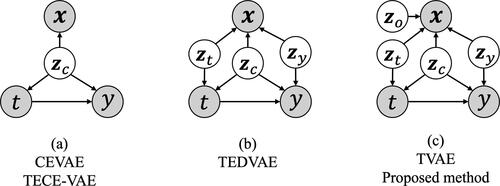
Table 1. Comparison of heterogeneous treatment effect estimation methods based on the VAE.

Method	Number of latent factors	Type of treatment covered
	single	multiple	binary	continuous
CEVAE	1	✓		✓
TEDVAE	3	✓		✓
TVAE	4	✓		✓
TECE-VAE	1	✓	✓	✓
Proposed Method	4	✓	✓	✓	✓

In addition to the proposed method and TECE-VAE, there are several heterogeneous treatment effect estimation methods based on deep learning that can estimate multiple treatments. Yoon et al. (2018) used a generative adversarial network (GAN) (Goodfellow et al., 2020) approach to estimate treatment effects when there are multiple treatments and generative adversarial nets for inference of individualized treatment effects (GANITE). Zhao and Harinen (2019) also adapted X-learner and R-learner to multiple treatments and proposed extending X-Learner and R-Learner for multiple treatments. However, these treatments are defined as categorical variables and treatments are not expressed as a combination of multiple treatments using vectors, as in the proposed method. Therefore, even if each treatment has common content, it is learned as an independent treatment. Therefore, it is impractical to use these methods in situations where there are many possible treatment implementation patterns, including continuous treatment. Schwab et al. (2020) proposed a dose response network (DRNet) that learns the counterfactual virtual representations of treatments with continuous parameters. This method and the proposed method are the same in that the treatment is estimated as a continuous variable, allowing the treatment effect that had not been implemented in the past to be estimated as well. However, DRNet differs in that it estimates the effect of changing parameters in a treatment with one continuous parameter. Because the proposed method represents treatments as vectors, it is possible to estimate treatment effects by mixing binary treatments and expressing the treatments using continuous parameters.

2.2. Problem formulation

${\mathit{x}}_i\sim p(\mathit{x})\in {\mathbb{R}}^{\mathit{m}}$ represents the m -dimensional pretreatment covariates for individual i assigned factual K types of treatments ${\mathit{t}}_i=[t_{i1},\dots ,t_{\mathit{\text{ik}}},\dots ,t_{\mathit{\text{iK}}}]\sim p(\mathit{t}|\mathit{x})$ resulting in outcome $y_i\sim p(y|\mathit{x},\mathit{t}).$ Note that t_ik is $t_{\mathit{\text{ik}}}\in \{0,1\}$ when t_ik is a binary variable and $t_{\mathit{\text{ik}}}\sim \in \mathbb{R}$ when it is a continuous variable. These constitute the dataset $D={[y_i,{\mathit{t}}_i,{\mathit{x}}_i]}_{i=1}^N$ where N is the sample size. This setting is a direct extension of the Rubin-Neyman potential outcome framework (Rubin, 2005).

This study assumes that the following three assumptions (Rosenbaum & Rubin, 1983) regarding treatment effect estimation are satisfied. (1) Stable unit treatment value assumption (STUVA): The potential outcome for an individual is unaffected by the treatment of others. (2) Unconfoundedness: The treatment distribution is independent of the potential outcome when conditioning the observed variables. (3) Overlap: Every individual has a nonzero probability of receiving either treatment or control when given the observed variables. Although clear indicators must be defined for treatment effects, the average treatment effect (ATE) and conditional average treatment effect (CATE) are the two main indicators [37]. The ATE is the difference in the mean values of the outcome between a treatment and control group, which indicates an average causal effect on the entire group. The CATE represents the average treatment effect in a group with the same covariate values. In our study, we focused on estimating the CATE for multiple treatments. For example, if only the first of the three binary treatments is implemented for a user, ${\mathit{t}}_i=[1,0,0],$ the CATE =$E[y_i|{\mathit{x}}_i,{\mathit{t}}_i=[1,0,0]]-E[y_i|{\mathit{x}}_i,{\mathit{t}}_i=[0,0,0]].$ Here, $\mathit{\text{do}}({\mathit{t}}_i={\mathit{t}}^{\prime })$ indicates that intervening at ${\mathit{t}}_i$ and setting it to a given static or dynamic value or distribution eliminates its original dependency (Pearl, 2009).

3. Proposed method

3.1. Model overview

In this paper, we propose a method to estimate the CATE for multiple treatments and derive treatments that are considered optimal for each user by targeting observational data in recent business activities and elsewhere. We assume that observational data generally accumulated in recent business activities and elsewhere have the following characteristics.

1. Treatments are not assigned randomly.

2. Multiple treatments are implemented.

3. Even the same treatments have different effects on different users.

4. Diverse causal relationships are inherent.

5. Treatments with continuous parameters are implemented, such as discount amounts in coupon distribution.

The proposed method is a model based on the TECE-VAE that can deal with characteristics I-III. The proposed method also assumes a causal graph, as represented by (c) in Figure 2. In addition, the proposed method learns two types of treatment: one generated from a Bernoulli distribution and another from a normal distribution. By learning in this way, the CATE can be estimated for characteristics I-V, considering various causal relationships in the real world and treating the content of treatments that are continuous in nature as continuous variables. The overall architecture of the proposed method is shown in Figure 2. Here, we assume that covariates $\mathit{x}$ can be viewed as generated from four disjoint sets of latent factors $\mathit{z}=({\mathit{z}}_c,{\mathit{z}}_y,{\mathit{z}}_t,{\mathit{z}}_o).$ ${\mathit{z}}_c$ are confounding factors that affect both the treatment and outcome, ${\mathit{z}}_y$ are factors that affect only the outcome, and ${\mathit{z}}_t$ are factors that affect only the treatment. Meanwhile, ${\mathit{z}}_o$ are unrelated to treatment and/or outcomes. By decomposing it in this manner, we aim to satisfy the unboundedness assumption for observational data with diverse inherent causal relationships.

Figure 2. Overall architecture of the proposed method. The white nodes represent the parameterized neural network transitions, and the gray nodes represent the extraction of samples from a probability distribution. The white circles represent the inner product.

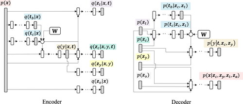
3.2. Encoder

The proposed method is a deep generative model consisting of an encoder and decoder. In this section, the encoder is described. In the encoder, we recover the distribution of the latent factors $\mathit{z}=({\mathit{z}}_c,{\mathit{z}}_y,{\mathit{z}}_t,{\mathit{z}}_o).$ First, the encoder inputs the covariate vector $\mathit{x}$ and estimates the probability distribution of the treatment implementation vector ${\mathit{t}}_b$ for the binary variable and treatment implementation vector ${\mathit{t}}_c$ for the continuous variable from each parameter obtained. Here, $q({\mathit{t}}_b|\mathit{x})$ and $q({\mathit{t}}_c|\mathit{x})$ are defined by equations (1)-(2), respectively. Note that $K_{{\mathit{t}}_b}$ is the number of treatments for binary variables, $K_{{\mathit{t}}_c}$ is the number of treatments for continuous variables, $q_B(·)$ is the probability mass function of the Bernoulli distribution, $q_N(·)$ is the probability density function of the normal distribution, ${\pi }_{{\mathit{t}}_{b_q}}^{(k)}$ is the parameter of the mean included in the Bernoulli distribution for the elements of ${\mathit{t}}_b$ obtained in the previous layer, and ${\mu }_{{\mathit{t}}_{c_q}}^{(k)},{\sigma }_{{\mathit{t}}_{c_q}}^{{(k)}^2}$ are the mean and variance parameters contained in the normal distribution for the elements of ${\mathit{t}}_c$ obtained in the previous layer. (1) $$q({\mathit{t}}_b|\mathit{x})=\prod _{k=1}^{K_{{\mathit{t}}_b}}{q}_B(t_{\mathit{\text{bk}}}|{\pi }_{{\mathit{t}}_{b_q}}^{(k)})$$(1) (2) $$q({\mathit{t}}_c|\mathit{x})=\prod _{k=1}^{K_{{\mathit{t}}_c}}{q}_N(t_{\mathit{\text{ck}}}|{\mu }_{{\mathit{t}}_{c_q}}^{(k)},{\sigma }_{{\mathit{t}}_{c_q}}^{{(k)}^2})$$(2)

Subsequently, we concatenate sampled ${\tilde{\mathit{t}}}_b\in {\{0,1\}}^{K_{{\mathit{t}}_b}}$ and ${\tilde{\mathit{t}}}_c\in {\mathbb{R}}^{K_{{\mathit{t}}_c}}$ to form $\tilde{\mathit{t}}\in {\mathbb{R}}^{K_{\mathit{t}}}.$ Note that $K_{\mathit{t}}=K_{{\mathit{t}}_b}+K_{{\mathit{t}}_c}.$ $\tilde{\mathit{t}}$ and the embedding matrix W $\in {\mathbb{R}}^{K_{\mathit{t}}\times K_{\mathit{W}}},$ we calculate $\mathit{\tau }\in {\mathbb{R}}^{K_{\mathit{W}}}$ as expressed by (3)(3) $$q(y|\mathit{x},\mathit{t})=q_N(y|{\mu }_{y_q},{\sigma }_{y_q}^2)$$(3) . (3) $$\mathit{\tau }=\mathbf{W}{\tilde{\mathit{t}}}^{\top }$$(3)

After calculating $\mathit{\tau },$ we estimate $q(y|\mathit{x},\mathit{t})$ defined in (3)(3) $$q(y|\mathit{x},\mathit{t})=q_N(y|{\mu }_{y_q},{\sigma }_{y_q}^2)$$(3) from $\mathit{x}$ and $\mathit{\tau }$ and then sample $\tilde{y}$ from the obtained distribution. Here, ${\mu }_{y_q}$ and ${\sigma }_{y_q}^2$ denote the mean and variance parameters, respectively, in the normal distribution for y obtained in the previous layer. (3) $$q(y|\mathit{x},\mathit{t})=q_N(y|{\mu }_{y_q},{\sigma }_{y_q}^2)$$(3)

Finally, using $\mathit{x},\mathit{\tau }$ and $\tilde{y},$ we estimate $q({\mathit{z}}_c|\mathit{x},y,\mathit{t}),q({\mathit{z}}_y|\mathit{x},y),q({\mathit{z}}_t|\mathit{x},\mathit{t}),q({\mathit{z}}_o|\mathit{x})$ by the following (5)(5) $$q({\mathit{z}}_c|\mathit{x},y,\mathit{t})=\prod _{d=1}^{D_{{\mathit{z}}_c}}{q}_N(z_{\mathit{\text{cd}}}|{\mu }_{{\mathit{z}}_c}^{(d)},{\sigma }_{{\mathit{z}}_c}^{{(d)}^2})$$(5) -(8)(8) $$q({\mathit{z}}_o|\mathit{x})=\prod _{d=1}^{D_{{\mathit{z}}_o}}{q}_N(z_{\mathit{\text{od}}}|{\mu }_{{\mathit{z}}_o}^{(d)},{\sigma }_{{\mathit{z}}_o}^{{(d)}^2})$$(8) . Note that $D_{{\mathit{z}}_c},D_{{\mathit{z}}_y},D_{{\mathit{z}}_t},$ and $D_{{\mathit{z}}_o}$ denote the number of dimensions of latent variable ${\mathit{z}}_c,$ number of dimensions of latent variable ${\mathit{z}}_y,$ number of dimensions of latent variable ${\mathit{z}}_t,$ and number of dimensions of latent variable ${\mathit{z}}_o,$ respectively. Moreover, ${\mu }_{{\mathit{z}}_c}^{(d)},{\sigma }_{{\mathit{z}}_c}^{{(d)}^2},{\mu }_{{\mathit{z}}_y}^{(d)},{\sigma }_{{\mathit{z}}_y}^{{(d)}^2},{\mu }_{{\mathit{z}}_t}^{(d)},{\sigma }_{{\mathit{z}}_t}^{{(d)}^2},{\mu }_{{\mathit{z}}_o}^{(d)}$ and ${\sigma }_{{\mathit{z}}_o}^{{(d)}^2}$ are the mean and variance parameters included in the normal distribution for ${\mathit{z}}_c,{\mathit{z}}_y,{\mathit{z}}_t$ and ${\mathit{z}}_o$ calculated for the d-th element in each vector. (5) $$q({\mathit{z}}_c|\mathit{x},y,\mathit{t})=\prod _{d=1}^{D_{{\mathit{z}}_c}}{q}_N(z_{\mathit{\text{cd}}}|{\mu }_{{\mathit{z}}_c}^{(d)},{\sigma }_{{\mathit{z}}_c}^{{(d)}^2})$$(5) (6) $$q({\mathit{z}}_y|\mathit{x},y)=\prod _{d=1}^{D_{{\mathit{z}}_y}}{q}_N(z_{\mathit{\text{yd}}}|{\mu }_{{\mathit{z}}_y}^{(d)},{\sigma }_{{\mathit{z}}_y}^{{(d)}^2})$$(6) (7) $$q({\mathit{z}}_t|\mathit{x},\mathit{t})=\prod _{d=1}^{D_{{\mathit{z}}_t}}{q}_N(z_{\mathit{\text{td}}}|{\mu }_{{\mathit{z}}_t}^{(d)},{\sigma }_{{\mathit{z}}_t}^{{(d)}^2})$$(7) (8) $$q({\mathit{z}}_o|\mathit{x})=\prod _{d=1}^{D_{{\mathit{z}}_o}}{q}_N(z_{\mathit{\text{od}}}|{\mu }_{{\mathit{z}}_o}^{(d)},{\sigma }_{{\mathit{z}}_o}^{{(d)}^2})$$(8)

3.3. Decoder

First, we define the prior distributions $p({\mathit{z}}_c),p({\mathit{z}}_y),p({\mathit{z}}_t),$ and $p({\mathit{z}}_o)$ as in (9)(9) $$p({\mathit{z}}_{\{c,y,t,o\}})=\prod _{d=1}^{D_{\{{\mathit{z}}_c,{\mathit{z}}_y,{\mathit{z}}_t,{\mathit{z}}_o\}}}{p}_N(z_{\{c,y,t,o\}d}|0,1)$$(9) . The latent factors $\mathit{z}=({\mathit{z}}_c,{\mathit{z}}_y,{\mathit{z}}_t,{\mathit{z}}_o)$ are assumed to be vectors of the independent, univariate normal variables. Let $p_N(·)$ be the probability density function of a normal distribution. (9) $$p({\mathit{z}}_{\{c,y,t,o\}})=\prod _{d=1}^{D_{\{{\mathit{z}}_c,{\mathit{z}}_y,{\mathit{z}}_t,{\mathit{z}}_o\}}}{p}_N(z_{\{c,y,t,o\}d}|0,1)$$(9)

Second, we estimate $p({\mathit{t}}_b|{\mathit{z}}_c,{\mathit{z}}_t)$ and $p({\mathit{t}}_c|{\mathit{z}}_c,{\mathit{z}}_t)$ from ${\mathit{z}}_c$ and ${\mathit{z}}_t$ expressed by (10)(10) $$p({\mathit{t}}_b|{\mathit{z}}_c,{\mathit{z}}_t)=\prod _{k=1}^{K_{{\mathit{t}}_b}}{p}_B(t_{\mathit{\text{bk}}}|{\pi }_{{\mathit{t}}_{b_p}}^{(k)})$$(10) -(11)(11) $$p({\mathit{t}}_c|{\mathit{z}}_c,{\mathit{z}}_t)=\prod _{k=1}^{K_{{\mathit{t}}_c}}{p}_N(t_{\mathit{\text{ck}}}|{\mu }_{{\mathit{t}}_{c_p}}^{(k)},{\sigma }_{{\mathit{t}}_{c_p}}^{{(k)}^2})$$(11) and then calculate $\mathit{\tau }$ in the same manner as for the encoder using $\tilde{\mathit{t}},$ which is the concatenation of the sampled ${\tilde{\mathit{t}}}_b$ and ${\tilde{\mathit{t}}}_c.$ Note that $p_B(·)$ is the probability mass function of the Bernoulli distribution, ${\pi }_{{\mathit{t}}_{b_p}}^{(k)}$ is the parameter of the mean included in the Bernoulli distribution for the elements of ${\mathit{t}}_b$ obtained in the previous layer, and ${\mu }_{{\mathit{t}}_{c_p}}^{(k)},{\sigma }_{{\mathit{t}}_{c_p}}^{{(k)}^2}$ are the mean and variance parameters contained in the normal distribution for the elements of ${\mathit{t}}_c$ obtained in the previous layer. (10) $$p({\mathit{t}}_b|{\mathit{z}}_c,{\mathit{z}}_t)=\prod _{k=1}^{K_{{\mathit{t}}_b}}{p}_B(t_{\mathit{\text{bk}}}|{\pi }_{{\mathit{t}}_{b_p}}^{(k)})$$(10) (11) $$p({\mathit{t}}_c|{\mathit{z}}_c,{\mathit{z}}_t)=\prod _{k=1}^{K_{{\mathit{t}}_c}}{p}_N(t_{\mathit{\text{ck}}}|{\mu }_{{\mathit{t}}_{c_p}}^{(k)},{\sigma }_{{\mathit{t}}_{c_p}}^{{(k)}^2})$$(11)

Finally, we estimate $p(y|\mathit{t},{\mathit{z}}_c,{\mathit{z}}_y),$ defined in (12), using ${\mathit{z}}_c,{\mathit{z}}_y,$ and $\mathit{\tau }.$ We also estimate $p(\mathit{x}|{\mathit{z}}_c,{\mathit{z}}_y,{\mathit{z}}_t,{\mathit{z}}_o)$ as defined in (13)(13) $$p(\mathit{x}|{\mathit{z}}_c,{\mathit{z}}_y,{\mathit{z}}_t,{\mathit{z}}_o)=\prod _{j=1}^{J}p(x_j|{\mathit{z}}_c,{\mathit{z}}_y,{\mathit{z}}_t,{\mathit{z}}_o)$$(13) from all latent variables ${\mathit{z}}_c,{\mathit{z}}_y,{\mathit{z}}_t$ and ${\mathit{z}}_o.$ Note that ${\mu }_{y_p}$ and ${\sigma }_{y_p}^2$ denote the mean and variance parameters in the normal distribution for y obtained in the previous layer. Further, J denotes the dimensionality of the covariate $\mathit{x}$ and we let $p(x_j|{\mathit{z}}_c,{\mathit{z}}_y,{\mathit{z}}_t,{\mathit{z}}_o)$ be an appropriate distribution for the j-th covariate. (12) $$p(y|\mathit{t},{\mathit{z}}_c,{\mathit{z}}_y)=p_N(y|{\mu }_{y_p},{\sigma }_{y_p}^2)$$(12) (13) $$p(\mathit{x}|{\mathit{z}}_c,{\mathit{z}}_y,{\mathit{z}}_t,{\mathit{z}}_o)=\prod _{j=1}^{J}p(x_j|{\mathit{z}}_c,{\mathit{z}}_y,{\mathit{z}}_t,{\mathit{z}}_o)$$(13)

3.4. Objective function

Using the variational lower bound $\mathcal{L}(\mathit{x},y,\mathit{t}),$ expressed by (14)(14) $$\begin{array}{c}\mathcal{L}(\mathit{x},y,\mathit{t})=\\ {\mathbb{E}}_{q({\mathit{z}}_c|\mathit{x},y,\mathit{t})q({\mathit{z}}_y|\mathit{x},y)q({\mathit{z}}_t|\mathit{x},\mathit{t})q({\mathit{z}}_o|\mathit{x})}[\mathrm{\text{log}}\hspace{0.17em}p(\mathit{x}|{\mathit{z}}_c,{\mathit{z}}_y,{\mathit{z}}_t,{\mathit{z}}_o)+\hspace{0.17em}\mathrm{\text{log}}\hspace{0.17em}p(y|\mathit{t},{\mathit{z}}_c,{\mathit{z}}_y)\\ +\hspace{0.17em}\mathrm{\text{log}}\hspace{0.17em}p({\mathit{t}}_b|{\mathit{z}}_c,{\mathit{z}}_t)+\hspace{0.17em}\mathrm{\text{log}}\hspace{0.17em}p({\mathit{t}}_c|{\mathit{z}}_c,{\mathit{z}}_t)]\\ -D_{\mathit{\text{KL}}}[q({\mathit{z}}_c|\mathit{x},y,\mathit{t})\left|\right|p({\mathit{z}}_c)]\\ -D_{\mathit{\text{KL}}}[q({\mathit{z}}_y|\mathit{x},y)\left|\right|p({\mathit{z}}_y)]\\ -D_{\mathit{\text{KL}}}[q({\mathit{z}}_t|\mathit{x},\mathit{t})\left|\right|p({\mathit{z}}_t)]\\ -D_{\mathit{\text{KL}}}[q({\mathit{z}}_o|\mathit{x})\left|\right|p({\mathit{z}}_o)]\\ \end{array}$$(14) , the objective function of the proposed method $\mathcal{F}$ is expressed by (15)(15) $$\begin{array}{c}\mathcal{F}=\\ \mathcal{L}(\mathit{x},y,\mathit{t})+{\mathbb{E}}_{q({\mathit{z}}_c|\mathit{x},y,\mathit{t})q({\mathit{z}}_y|\mathit{x},y)q({\mathit{z}}_t|\mathit{x},\mathit{t})q({\mathit{z}}_o|\mathit{x})}[\mathrm{\text{log}}\hspace{0.17em}q({\mathit{t}}_b={\mathit{t}}_b^{*}|{\mathit{x}}^{*})+\hspace{0.17em}\mathrm{\text{log}}\hspace{0.17em}q({\mathit{t}}_c={\mathit{t}}_c^{*}|{\mathit{x}}^{*})\\ +\hspace{0.17em}\mathrm{\text{log}}\hspace{0.17em}q(y=y^{*}|{\mathit{x}}^{*},{\mathit{t}}^{*})]\end{array}$$(15) . (14) $$\begin{array}{c}\mathcal{L}(\mathit{x},y,\mathit{t})=\\ {\mathbb{E}}_{q({\mathit{z}}_c|\mathit{x},y,\mathit{t})q({\mathit{z}}_y|\mathit{x},y)q({\mathit{z}}_t|\mathit{x},\mathit{t})q({\mathit{z}}_o|\mathit{x})}[\mathrm{\text{log}}\hspace{0.17em}p(\mathit{x}|{\mathit{z}}_c,{\mathit{z}}_y,{\mathit{z}}_t,{\mathit{z}}_o)+\hspace{0.17em}\mathrm{\text{log}}\hspace{0.17em}p(y|\mathit{t},{\mathit{z}}_c,{\mathit{z}}_y)\\ +\hspace{0.17em}\mathrm{\text{log}}\hspace{0.17em}p({\mathit{t}}_b|{\mathit{z}}_c,{\mathit{z}}_t)+\hspace{0.17em}\mathrm{\text{log}}\hspace{0.17em}p({\mathit{t}}_c|{\mathit{z}}_c,{\mathit{z}}_t)]\\ -D_{\mathit{\text{KL}}}[q({\mathit{z}}_c|\mathit{x},y,\mathit{t})\left|\right|p({\mathit{z}}_c)]\\ -D_{\mathit{\text{KL}}}[q({\mathit{z}}_y|\mathit{x},y)\left|\right|p({\mathit{z}}_y)]\\ -D_{\mathit{\text{KL}}}[q({\mathit{z}}_t|\mathit{x},\mathit{t})\left|\right|p({\mathit{z}}_t)]\\ -D_{\mathit{\text{KL}}}[q({\mathit{z}}_o|\mathit{x})\left|\right|p({\mathit{z}}_o)]\\ \end{array}$$(14) (15) $$\begin{array}{c}\mathcal{F}=\\ \mathcal{L}(\mathit{x},y,\mathit{t})+{\mathbb{E}}_{q({\mathit{z}}_c|\mathit{x},y,\mathit{t})q({\mathit{z}}_y|\mathit{x},y)q({\mathit{z}}_t|\mathit{x},\mathit{t})q({\mathit{z}}_o|\mathit{x})}[\mathrm{\text{log}}\hspace{0.17em}q({\mathit{t}}_b={\mathit{t}}_b^{*}|{\mathit{x}}^{*})+\hspace{0.17em}\mathrm{\text{log}}\hspace{0.17em}q({\mathit{t}}_c={\mathit{t}}_c^{*}|{\mathit{x}}^{*})\\ +\hspace{0.17em}\mathrm{\text{log}}\hspace{0.17em}q(y=y^{*}|{\mathit{x}}^{*},{\mathit{t}}^{*})]\end{array}$$(15)

Note that ${\mathit{t}}_b^{*}$ and ${\mathit{t}}_c^{*}$ represent the treatment implementation vectors of the binary and continuous variables in the training data, respectively. ${\mathit{t}}^{*}$ is the concatenation of ${\mathit{t}}_b^{*}$ and ${\mathit{t}}_c^{*}.$

4. Simulation experiment

This section describes experiments conducted on artificial datasets to investigate the ability of the proposed method to infer latent factors and estimate treatment effects. We extended the dataset called TVAESynth (Vowels et al., 2021) and used it for our evaluation experiments. Specifically, two types of situations were envisaged. One is a situation in which all treatments were binary and the other was where the binary and continuous treatments were mixed.

4.1. Experimental setup

4.1.1. Synthetic datasets

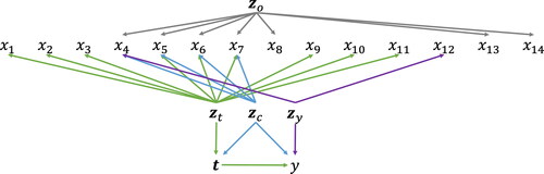
We used an artificial dataset that was generated from the structure illustrated in Figure 3 and equations (16)-(19), where (a) is used in Setting A and (b) in Setting B. Both (a) and (b) assume three types of treatment. The treatments are all binary in Setting A, and there are one continuous treatment and two binary treatments in Setting B. The number of training and test data samples was 90,000 and 10,000, respectively. (16) $$\begin{array}{c}{\mathit{U}}_{z_c,z_y,z_{t_1},z_{t_2},z_{t_3},z_o,y}\sim \mathcal{N}(\mathit{0},\mathit{1})\\ {\mathit{U}}_{x_{1:3},x_8,t_1,t_2,t_3}\sim \mathit{\text{Bern}}(0.5)\\ {\mathit{U}}_{x_4,x_{5:7},x_{9:11},x_{12},x_{13},x_{14}}\sim \mathcal{N}(\mathit{0},\mathit{1})\\ z_c=U_{z_c}\\ z_y=U_{z_y}\\ z_{t_1}=U_{z_{t_1}}\\ z_{t_2}=U_{z_{t_2}}\\ z_{t_3}=U_{z_{t_3}}\\ z_o=U_{z_o}\end{array}$$(16) (17) $$\begin{array}{c}{x}_1\sim \mathit{\text{Bern}}(\sigma (z_{t_1}+0.1(U_{x_{1:3}}-0.5)))\\ x_2\sim \mathit{\text{Bern}}(\sigma (z_{t_2}+0.1(U_{x_{1:3}}-0.5)))\\ x_3\sim \mathit{\text{Bern}}(\sigma (z_{t_3}+0.1(U_{x_{1:3}}-0.5)))\\ x_4\sim \mathcal{N}(0.4z_o+0.3z_c+0.5z_y+0.1U_{x_4},0.2)\\ x_5\sim \mathcal{N}(0.2z_o+0.2z_c+1.2z_{t_1}+0.1U_{x_{5:7}},0.2)\\ x_6\sim \mathcal{N}(0.2z_o+0.2z_c+1.2z_{t_2}+0.1U_{x_{5:7}},0.2)\\ x_7\sim \mathcal{N}(0.2z_o+0.2z_c+1.2z_{t_3}+0.1U_{x_{5:7}},0.2)\\ x_8\sim \mathit{\text{Bern}}(\sigma (0.6z_o+0.1(U_{x_8}-0.5)))\\ x_9\sim \mathcal{N}(0.6z_{t_1}+0.1U_{x_{9:11}},0.1)\\ x_{10}\sim \mathcal{N}(0.6z_{t_2}+0.1U_{x_{9:11}},0.1)\\ x_{11}\sim \mathcal{N}(0.6z_{t_3}+0.1U_{x_{9:11}},0.1)\\ x_{12}\sim \mathcal{N}(0.9z_y+0.1U_{x_{12}},0.1)\\ x_{13}\sim \mathcal{N}(0.5z_o+0.1U_{x_{13}},0.1)\\ x_{14}\sim \mathcal{N}(0.5z_o+0.1U_{x_{14}},0.1)\end{array}$$(17) (18) $$\begin{array}{c}{t}_1\sim \mathit{\text{Bern}}(\sigma (0.2z_c+0.8z_{t_1}+0.1U_{t_1}))\\ t_2\sim \mathit{\text{Bern}}(\sigma (0.2z_c+0.8z_{t_2}+0.1U_{t_2}))\\ t_{3b}\sim \mathit{\text{Bern}}(\sigma (0.2z_c+0.8z_{t_3}+0.1U_{t_3}))\\ t_{3c}\sim \mathcal{N}(0.2z_c+0.8z_{t_3}+0.1U_{t_3},0.1)\\ (a):\mathit{t}=[t_1,t_2,t_3]=[t_1,t_2,t_{3b}]\\ (b):\mathit{t}=[t_1,t_2,t_3]=[t_1,t_2,t_{3c}]\end{array}$$(18) (19) $$\begin{array}{c}y:=0.2z_c+0.5z_y+0.2(z_y+1)(t_1+t_2+t_3)\\ +0.03(z_y+1)(t_1{t}_2+t_2{t}_3+t_1{t}_3)\\ +0.01(z_y+1)t_1{t}_2{t}_3+0.1U_y\end{array}$$(19)

Figure 3. Data structure of the artificial dataset.

4.1.2. Baselines

As a baseline, we used random forest (RF) (Breiman, 2001), gradient boosting machine (GBM) (Friedman, 2001), DragonNet (Shi et al., 2019), and extending R-learner using random forest algorithms as the base learner (R-RF) (Zhao & Harinen, 2019). We also used the conventional method TECE-VAE, after modifying the model to be able to estimate the treatment of continuous variables, as in the improvement of the proposed method. This is to verify differences in estimation accuracy due to different causal graphs. GANITE was excluded from the baseline because codes for multiple treatment estimations were unavailable. Python libraries scikit-learn (Pedregosa et al., 2011) and CausalML (Chen et al., 2020) were used to implement RF, GBM and DragonNet, R-RF, respectively. Tensorflow (Abadi et al., 2011) and Edward (Tran et al., 2017) were used for the implementation of the TECE-VAE and proposed method.

Here, TEDVAE and TVAE, which are similar models to the proposed method, are not used as baselines because they are models used in a different problem setting than the proposed method. Specifically, TEDVAE and TVAE are used to estimate the effect of binary treatments, whereas our method is designed to estimate the effect of multiple treatments. Therefore, although their methods are similar to ours, they are not used as a baseline in the current artificial dataset, which assumes the estimation of effects in the case of multiple treatments.

RF and GBM are not methods originally proposed for estimating causal effects and cannot be directly applied to multiple treatment settings using treatment as a vector. Therefore, as in Yoon et al. (2018), we considered all possible subsets of treatments to be separate treatments and encoded them as one-hot vectors. There are $2^k$ distinct treatment subsets; thus, the size of the one-hot vector is $2^k.$ The $2^k$ one-treatment effect estimates can be regarded as multiple-treatment effect estimates, and the final number of models must be $2^k.$ However, in this way, causal effects in multiple treatment settings can be estimated using RF and GBM to classify and predict outcomes.

Furthermore, it is impractical to use DragonNet and R-RF in situations where there are many possible treatment implementation patterns, including continuous treatment. Therefore, these estimate the effect of measures only in Setting A, which assumes only binary treatments. In the proposed method and TECE-VAE, the number of dimensions of the latent variables ${\mathit{z}}_c,{\mathit{z}}_y,$ and ${\mathit{z}}_t$ was four, and the number of dimensions of latent variables ${\mathit{z}}_o$ was two. However, to consider the relationship between the causal graph and the number of latent variables, in the TECE-VAE method, ${\mathit{z}}_c$ was tested using three patterns (4, 20, and 40). The number of dimensions of the embedding matrix $\mathit{W}$ was 10, and 200 hidden neurons were used with two layers and ELU activation (Clevert et al., 2016). Early stopping was set to 30, and the learning rate was set to $1\times {10}^{-5}.$ All models were optimized using Adam (Kingma & Ba, 2017).

4.1.3. Evaluation criteria

To evaluate the performance of CATE estimation, we used the precision in estimation of heterogeneous effect (PEHE) (Hill, 2011) for 50 trials for each condition. PEHE represents the error in CATE calculated on a per-individual basis. Our proposed method aims at estimating effects in individuals. Therefore, it is appropriate to evaluate the accuracy of the estimation using PEHE, and although it is possible to evaluate even the error of the ATE, which indicates an average causal effect on the entire group, this is not the purpose of the original proposed method and is therefore omitted. PEHE is expressed by (20)(20) $${ϵ}_{\mathit{\text{PEHE}}}=\sqrt{\frac{1}{N}\sum _{i=1}^N{\left(\widehat{\tau }({\mathit{x}}_i)-\tau ({\mathit{x}}_i)\right)}^2}$$(20) . However, $\tau (\mathit{x})$ is the ground truth CATE for subjects with observed variables ${\mathit{x}}_i.$ (20) $${ϵ}_{\mathit{\text{PEHE}}}=\sqrt{\frac{1}{N}\sum _{i=1}^N{\left(\widehat{\tau }({\mathit{x}}_i)-\tau ({\mathit{x}}_i)\right)}^2}$$(20)

In the proposed method and TECE-VAE, 100 samples were drawn for each set of input covariates when estimating the treatment effects. For continuous treatment, we predicted CATE for the cases $t_3=\{-6,-3,-1,0,1,3,6\}.$ Here, $t_3=\{-6,6\}$ are extrapolations because the continuous treatment had a minimum value of -3.85 and a maximum value of 4.00 after sampling 1 million times.

4.2. Simulation results

4.2.1. Setting A (three binary treatments)

Table 2 shows the mean and standard deviation of PEHE for 50 runs for each condition, when all treatments were binary. Table 2 shows that the proposed method has the lowest PEHE under all conditions and shows consistently high accuracy in all treatment implementation patterns. In particular, the improvement rate of the proposed method tended to be higher in situations where multiple treatments were implemented. The PEHE of the proposed method is smaller than that of the TECE-VAE even when the number of latent variables in the TECE-VAE is larger than the total number of latent variables in the proposed method, showing the effect of the improved causal graph. In conclusion, by improving the causal model, the proposed method can realize an appropriate estimation of the effects of measures, while accurately capturing various causal relationships.

Table 2. Mean and standard deviation of PEHE for test data in Setting A.

	Treatment Implementation Pattern
Method	(1,0,0)	(0,1,0)	(0,0,1)
RF	0.076±.001	0.305±.004	0.586±.005
GBM	0.057±.004	0.271±.005	0.497±.005
DragonNet	0.295±.072	0.314±.071	0.297±.071
R-RF	2.781±.238	2.775±.378	2.781±.308
TECE-VAE* (${\mathit{z}}_c$= 4)	0.157±.019	0.155±.020	0.157±.019
TECE-VAE* (${\mathit{z}}_c$=20)	0.054±.002	0.054±.002	0.054±.003
TECE-VAE* (${\mathit{z}}_c$=40)	0.048±.003	0.048±.003	0.048±.003
Proposed Method	0.046±.003	0.047±.003	0.046±.003
	Treatment Implementation Pattern
Method	(1,1,0)	(0,1,1)	(1,0,1)	(1,1,1)
RF	0.318±.004	0.318±.004	0.318±.004	0.141±.002
GBM	0.240±.004	0.240±.004	0.240±.004	0.169±.004
DragonNet	0.468±.036	0.460±.026	0.469±.045	0.657±.012
R-RF	3.474±.245	3.561±.325	3.478±.358	4.351±.380
TECE-VAE* (${\mathit{z}}_c$= 4)	0.309±.040	0.309±.039	0.314±.038	0.466±.057
TECE-VAE* (${\mathit{z}}_c$=20)	0.101±.003	0.100±.003	0.101±.004	0.148±.005
TECE-VAE* (${\mathit{z}}_c$=40)	0.088±.003	0.089±.003	0.089±.004	0.134±.006
Proposed Method	0.087±.003	0.087±.003	0.087±.003	0.129±.005

* Original code modified for multiple treatments.

4.2.2. Setting B (two binary treatments and one continuous treatment)

Table 3 shows the mean and standard deviation of PEHE for 50 runs in each condition in a situation where binary and continuous treatments were mixed. Table 3 shows that the proposed method has the lowest PEHE under all conditions, as well as in Setting A. It shows consistently high accuracy for all treatment combinations. In addition, the extrapolation of $t_3=\{-6,6\}$ shows a particularly large improvement rate, indicating a significant advantage in terms of accuracy. This can be attributed to the improved robustness of the model due to the improvements made in causal model. Based on the above results and the results of Setting A, it was confirmed that the proposed method can accurately estimate the treatment effects for both binary and continuous treatments while accurately capturing the causal relationships between the variables influencing the treatment effects.

Table 3. Mean and standard deviation of PEHE for test data in Setting B.

Method	Treatment Implementation Pattern
	(1,0,0)	(0,1,0)	(0,0,1)	(1,1,0)
RF	0.076±.003	0.302±.007	0.640±.014	0.376±.013
GBM	0.066±.005	0.234±.008	0.516±.016	0.263±.014
TECE-VAE* (${\mathit{z}}_c$= 4)	0.137±.010	0.137±.010	0.186±.039	0.275±.019
TECE-VAE* (${\mathit{z}}_c$=20)	0.052±.018	0.052±.019	0.292±.039	0.101±.038
TECE-VAE* (${\mathit{z}}_c$=40)	0.093±.038	0.093±.038	0.215±.048	0.185±.077
Proposed Method	0.048±.003	0.048±.003	0.082±.010	0.092±.005
Method	Treatment Implementation Pattern
	(0,1,1)	(1,0,1)	(1,1,1)	(0,0,-1)
RF	0.376±.013	0.376±.013	0.181±.007	0.537±.003
GBM	0.263±.014	0.263±.014	0.181±.009	0.511±.009
TECE-VAE* (${\mathit{z}}_c$=4)	0.367±.033	0.361±.034	0.536±.036	0.196±.022
TECE-VAE* (${\mathit{z}}_c$=20)	0.306±.020	0.307±.020	0.326±.046	0.324±.012
TECE-VAE* (${\mathit{z}}_c$=40)	0.301±.043	0.299±.042	0.391±.109	0.268±.023
Proposed Method	0.123±.012	0.123±.011	0.165±.014	0.077±.004
Method	Treatment Implementation Pattern
	(1,1,-1)	(0,1,-1)	(1,0,-1)	(0,0,-3)
RF	0.107±.012	0.264±.014	0.264±.006	0.248±.019
GBM	0.092±.013	0.233±.015	0.233±.010	0.564±.023
TECE-VAE* (${\mathit{z}}_c$=4)	0.144±.023	0.055±.037	0.053±.044	0.812±.078
TECE-VAE* (${\mathit{z}}_c$=20)	0.279±.022	0.292±.041	0.293±.041	0.943±.087
TECE-VAE* (${\mathit{z}}_c$=40)	0.206±.045	0.182±.092	0.184±.088	0.962±.248
Proposed Method	0.055±.003	0.046±.006	0.048±.007	0.228±.013
Method	Treatment Implementation Pattern
	(1,1,-3)	(0,1,-3)	(1,0,-3)	(0,0,3)
RF	0.263±.028	0.521±.035	0.239±.019	0.440±.036
GBM	0.426±.030	0.684±.031	0.489±.028	0.360±.021
TECE-VAE* (${\mathit{z}}_c$=4)	0.394±.118	0.615±.092	0.614±.091	1.031±.079
TECE-VAE* (${\mathit{z}}_c$=20)	0.896±.161	0.931±.120	0.932±.120	0.809±.104
TECE-VAE* (${\mathit{z}}_c$=40)	0.739±.358	0.857±.297	0.860±.296	0.696±.245
Proposed Method	0.154±.022	0.184±.015	0.186±.016	0.254±.041
Method	Treatment Implementation Pattern
	(1,1,3)	(0,1,3)	(1,0,3)	(0,0,-6)
RF	0.399±.050	0.311±.046	0.311±.046	1.638±.040
GBM	0.745±.023	0.512±.011	0.512±.011	1.689±.034
TECE-VAE* (${\mathit{z}}_c$=4)	1.439±.119	1.263±.097	1.252±.095	1.903±.150
TECE-VAE* (${\mathit{z}}_c$=20)	0.860±.192	0.838±.154	0.839±.153	1.684±.140
TECE-VAE* (${\mathit{z}}_c$=40)	0.881±.400	0.792±.338	0.789±.334	2.063±.450
Proposed Method	0.333±.014	0.269±.023	0.269±.023	0.683±.048
Method	Treatment Implementation Pattern
	(1,1,-6)	(0,1,-6)	(1,0,-6)	(0,0,6)
RF	1.381±.017	1.663±.018	1.663±.018	0.647±.113
GBM	1.357±.018	1.640±.020	1.640±.020	0.689±.026
TECE-VAE* (${\mathit{z}}_c$=4)	1.507±.141	1.719±.140	1.720±.139	2.552±.229
TECE-VAE* (${\mathit{z}}_c$=20)	1.707±.191	1.695±.156	1.696±.156	1.547±.382
TECE-VAE* (${\mathit{z}}_c$=40)	1.872±.528	1.970±.485	1.973±.485	1.443±.721
Proposed Method	0.407±.034	0.530±.039	0.531±.039	0.555±.026
Method	Treatment Implementation Pattern
	(1,1,6)	(0,1,6)	(1,0,6)
RF	1.088±.033	0.816±.031	0.816±.031
GBM	1.241±.029	0.963±.027	0.963±.027
TECE-VAE* (${\mathit{z}}_c$=4)	2.923±.291	2.759±.262	2.747±.260
TECE-VAE* (${\mathit{z}}_c$=20)	1.647±.423	1.595±.410	1.597±.409
TECE-VAE* (${\mathit{z}}_c$=40)	1.683±.741	1.563±.741	1.559±.738
Proposed Method	0.937±.120	0.783±.116	0.782±.116

5. Actual data analysis

We applied the proposed method to a real dataset and analyzed the treatment effects on users to discuss and evaluate specific methods for practical applications. We used data related to banner advertising measures and purchase history from a fashion EC site provided by ZOZO Inc. (ZOZO, Inc, 2023). In this experiment, we analyzed the CATE related to the amount of purchases made by users who were members of the EC site during the implementation period of the targeted measures by distributing coupons via banner advertisements.

5.1. Analysis conditions

The data acquisition period for the banner advertisement data extended from August 1, 2021, to October 31, 2021, and the data acquisition period for purchase history data extended from May 1, 2021, to October 31, 2021. The number of users was 39,419, of which the number for whom the measures were not yet implemented was 17,854; outcome y was the number of purchases during the implementation period of the targeted measures, and the content of the implemented measures was represented by four types of $\mathit{t}$= [presence of conditions for obtaining coupons, display A, display B, the number of coupons distributed]. Only the number of coupons distributed was a continuous variable, while the remainder were binary variables. Note that two coupon amounts were distributed during the implementation period of this measure: JPY 500 and JPY 1,000. The covariate $\mathit{x}$ was based on the user’s attribute information, purchase history, and information on the implementation of other types of measures. In training the model, the number of dimensions of latent variables ${\mathit{z}}_c,{\mathit{z}}_y,$ and ${\mathit{z}}_t$ was 10, those of the latent variable ${\mathit{z}}_o$ and the embedding matrix W were 5 and 10, respectively, 500 hidden neurons were used with four layers, and ELU activation. The early stopping was set to 30, and the learning rate was set to $1\times {10}^{-5}.$ The optimization was performed using Adam. When estimating the treatment effects, 100 samples were drawn for each set of input covariates. We used the trained model to predict the CATE for each user for the continuous variable distributed coupon amount t⁴= {250,500,750,1000,1250,1500}.

5.2. Analysis results

5.2.1. Analysis of average CATE (overall user effectiveness) by discount amount

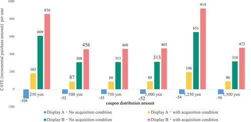
The average value of the estimated CATE for each treatment implementation pattern, estimated by training the model, is shown in Figure 4. Thus, it can be said that the marketing measure of coupon distribution by banner advertisement has different effects depending on the conditions under which the measures are implemented. Comparing the average value of CATE, display B was more effective. In addition, the measures with conditions for acquiring coupons were more effective. Comparing the average value of the CATE based on the number of coupons distributed, a particularly large effect was obtained when coupons worth JPY 250 and JPY 1,250 were distributed. This analysis suggests that distributing coupons worth JPY 1,250 may be the most effective, on average, based on the relationship between the coupon discount amount and profit, and that neither too large nor too small a discount is good. The fact that a coupon worth JPY 250 was found to be highly effective suggests that users tend to make purchases when they receive a coupon, even if it is a small amount.

Figure 4. Average value of the estimated CATE for each treatment implementation pattern.

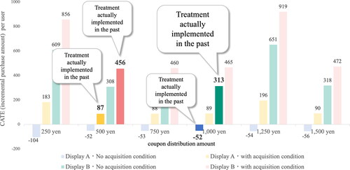
The results illustrated in Figure 4, broken down by past implementation of treatment, are shown in Figure 5. The light-colored graphs represent the effects of measures that have not yet been implemented. As shown in Figure 5, the measures in the data obtained for this analysis were not optimal on average, although they could be expected to be effective to some extent. Therefore, it is necessary to derive the most appropriate measures for each user in the future and consider implementing measures that have not yet been implemented.

Figure 5. Results of Figure 3 broken down by past implementation of treatment.

5.2.2. Proposal of optimal treatments for each user

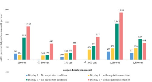
In this section, three examples were extracted to consider specific cases: User A, for whom a large CATE was estimated for a certain measure; User B, for whom the CATE was small for all measures; and User C, for whom the CATE was negative for all measures. In the following paragraphs, the characteristics of each user are discussed. Figure 6 shows the CATE of User A for each implementation pattern. From Figure 6, it is observed that User A has a large CATE in general, and among these, the measure with Display B, which has the conditions for acquiring a coupon and a coupon amount of JPY 1,250 to be distributed, has the largest effect. In other words, this user can be expected to have a sufficiently high effect in the future, and it is considered effective to take the above measures, which are expected to have the greatest effect among the estimated measures.

Figure 6. User A with large CATE estimated.

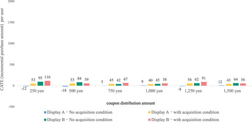
Figure 7 shows the CATE of User B for each implementation pattern of the measures. As shown in the figure, User B’s CATE is close to zero, indicating that the coupon distribution measure has almost no effect on this user. It can also be observed that the effect would be almost the same even if the treatment conditions were different. Therefore, these users are unlikely to make a purchase because of the coupon distribution and can be regarded as low-priority users for the implementation of measures. The actual number of measures to be taken up and the percentage of users that can be considered depends on the objectives and budget of the measures. The measure for the target data in this analysis is the distribution of coupons, which is expensive. Therefore, it is necessary to make an appropriate decision by comparing the CATE estimated by the proposed method with the cost, and it can be concluded that it is undesirable to implement measures for User B. However, it is not necessary that the purpose of the measures is always profit, and measures may be implemented for User B if the purpose is to increase public awareness.

Figure 7. User B with small CATE estimated.

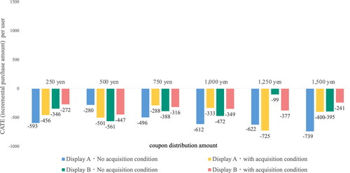
Figure 8 shows the CATE for each measure implementation pattern for User C. As shown in the figure, the effect of the measures is negative for all measures, indicating that the measures have the opposite effect. Clearly, the effect is almost the same, even if the measurement conditions are different. These users would have originally bought the products even without the coupon distribution. Since the effect of the measures was considered in terms of profit in this analysis, the CATE is considered to have become negative. This analysis considers the effect of the measures in terms of profit, which is thought to have resulted in a negative value for the CATE. Alternatively, users who were originally willing to buy the product may have withdrawn from the purchase because of aversion to the treatment. Therefore, it can be said that none of the measures should be implemented for such users. As described previously, the proposed method clarifies the most effective measures for each user and can estimate the effects of measures that have not been implemented in the past by changing the continuous value parameter. Thus, future marketing measures can be formulated based on the verification of effectiveness. Therefore, the proposed method is found to be practically useful.

Figure 8. User C with negative CATE estimated.

6. Discussion

Current measures used in EC sites tend to be implemented for users who are likely to defect from the site or are likely to receive measures predicted based on past observation data and the experience of marketers. For example, when distributing coupons as a marketing measure, the coupon usage rate is predicted for each user and measures are preferentially implemented for users who use coupons. However, this method of implementing measures cannot be considered appropriate from a business perspective, and it is desirable to identify the appropriate target group for the measures based on the treatment effect of coupon distribution. Against this background, when implementing measures, the results of the analysis using the proposed method based on past observation data can be used to estimate the measure effects for each user, which is expected to improve the cost-effectiveness of the measures. In addition, the proposed method can generate new measures that have not been implemented in the past by changing the parameters of the measures that can be handled by continuous variables and estimating their effects. Thus, the effects of many measures can be estimated even from limited data, thus reducing the cost of planning future marketing measures and future experiments.

Furthermore, although it is desirable to conduct an RCT to evaluate the effect of measures, it is difficult to conduct an RCT. Therefore, the proposed method targeting observational data is easy to use in businesses. In addition, the proposed method is practical because it is more applicable to the characteristics of observational data generally accumulated in companies than conventional methods. Because the proposed method can model the relationship between outcome variables, both discrete and continuous, it can estimate the impact of changing the number of discount coupons on the effectiveness of measures, which is useful for estimating the effectiveness of actual marketing measures.

In contrast, the proposed method is a deep generative model requiring a large amount of observation data. In general, statistical causal inference is often utilized in the fields of medical statistics and social sciences. However, the proposed method may not be suitable for such fields because of the amount of data required. Therefore, if you want to estimate CATE using a small number of data, it is recommended to use a tree-based method. In addition, it may be difficult to improve the proposed method to cope with small amounts of data and to make it practical. Although studies such as few-shot learning have been conducted, even if the proposed method is improved by utilizing these studies, it will not be superior to the tree-based method in terms of accuracy and interpretability. Therefore, at present, methods such as the proposed method are best suited to fields where large amounts of data can be obtained, such as EC marketing.

As the proposed method is a black box model, it is not suitable if the analysis of the factors that influence the effects of the measures is focused upon, rather than the selection of the most appropriate measures and users to implement the measures based on the effects of the measures. If the focus is on analyzing the factors influencing the effectiveness of the measures, a tree-based method should be used. The analysis of factors can also be considered in areas such as EC marketing. Therefore, analysts must consider whether to use the proposed method according to their objectives. If the proposed method is to also allow factor analysis in the future, it would be useful to refer to studies that add interpretability to VAE, given that the proposed method is based on VAE. Svensson et al. (2020) have successfully linearised parts of the VAE to increase interpretability, and our study should refer to such related research efforts.

7. Conclusion

In this study, an estimation method for treatment effects that can cope with situations where multiple types of treatment have been implemented, which can occur in business, and in situations where there is continuous treatment, such as coupon distribution, was proposed and implemented for the observed data of an EC site. In the proposed method, a graphical model with subdivided latent variables was constructed and a distribution is assumed for each type of treatment so that originally continuous treatments can be treated as continuous variables. In an evaluation experiment using an artificial dataset, it was shown that the proposed method can accurately estimate treatment effects for both binary and continuous variable treatments while accurately capturing the causal relationships between variables affecting the treatment effects. Furthermore, an analysis using a real dataset showed that the proposed method could identify the most effective treatment for each user. Additionally, because it is possible to estimate the effects of treatment parameters that have not been implemented in the past, it is possible to formulate future marketing treatments based on effectiveness verification. The results of this study have enabled the estimation of treatment effects from the observed data of an EC site, corresponding to situations in which multiple types of treatment, which can occur in business, and situations with continuous treatments, such as coupon distribution, have been implemented. This enables the design of various marketing treatments in real businesses and is expected to make a practical contribution.

Possible future work in this area is to implement the treatments that were found to be the most effective because of the effectiveness of estimation using the proposed method and to verify the effectiveness of the proposed method on these treatments.

By using a data-driven approach in an actual business, the effectiveness of the proposed method can be verified with more confidence. In addition, if only the proposed method is used and only the measures that are estimated to be the most effective are implemented, as described above, it is possible that the measures that are originally optimal may not be reached. This leads to problems related to reinforcement learning (Mnih et al., 2013) and bandit algorithms (Chapelle & Li, 2011). To gain new information and increase the accuracy of the model, it is suggested that it be performed stochastically and randomly or used in combination with an acquisition function, such as GP-UCP (Srinivas et al., 2009).

In addition, one important task is to devise a method for identifying covariates that influence the effect of measures to carry out more detailed analyses. As the proposed method is a treatment effect estimation method based on a deep generative model, it is not interpretable and therefore not very useful for analyzing factors influencing treatment effects. Therefore, it is desirable to devise a method that can identify covariates that influence treatment effects based on estimated treatment effects. For example, as a further extension of the proposed method, explainable (interpretable) artificial intelligence (Arrieta et al., 2020; Molnar, 2020), which explains the predictive basis of machine learning models, could solve this problem. In particular, the global surrogate model (Molnar, 2020), an explanation method that does not enter the internal structure of the model but focuses only on its input-output relationships, may be a good match as it is model-independent.

Disclosure statement

No potential conflict of interest was reported by the authors.

Additional information

Funding

This work was supported by JSPS KAKENHI (Grant Number 21H04600) and JST SPRING (Grant Number JPMJSP2128).

Appendix

Table A1. Notations used in this paper.

Notations	Descriptions
${\mathbb{R}}^{\mathit{m}}$	m-dimensional space
${\mathit{x}}_i$	covariates for individual i
yi	outcome for individual i
K	number of types of treatments
${\mathit{t}}_i=[t_{i1},\dots ,t_{\mathit{\text{ik}}},\dots ,t_{\mathit{\text{iK}}}]$	treatments for individual i
${\mathit{z}}_c$	latent factors that affect both treatment and outcome
${\mathit{z}}_y$	latent factors that affect only the outcome
${\mathit{z}}_t$	latent factors that affect only the treatment
${\mathit{z}}_o$	latent factors that are unrelated to the treatment
	and/or outcome
$K_{{\mathit{t}}_b}$	number of treatments for binary variables
$K_{{\mathit{t}}_c}$	number of treatments for continuous variables
$K_{\mathit{t}}$	$K_{{\mathit{t}}_b}+K_{{\mathit{t}}_c}$
$q_B(·)$	probability mass function of the Bernoulli distribution
$q_N(·)$	probability density function of the normal distribution
${\pi }_{{\mathit{t}}_b}^{(k)}$	parameter of the mean included in the Bernoulli
	distribution for the elements of ${\mathit{t}}_b$ obtained in the
	previous layer
${\mu }_{{\mathit{t}}_c}^{(k)}$	mean parameters contained in the normal distribution
	for the elements of ${\mathit{t}}_c$ obtained in the previous layer
${\sigma }_{{\mathit{t}}_c}^{{(k)}^2}$	variance parameters contained in the normal
	distribution for the elements of ${\mathit{t}}_c$ obtained in the
	previous layer
W	embedding matrix
μy	mean parameters in the normal distribution
	for y obtained in the previous layer
${\sigma }_y^2$	variance parameters in the normal distribution
	for y obtained in the previous layer
$D_{\mathit{z}}$	number of dimensions of latent variable $\mathit{z}$
${\mu }_{\mathit{z}}^{(d)}$	mean parameter included in the normal distribution for
	$\mathit{z}$ calculated for the d-th element in each vector
${\sigma }_{\mathit{z}}^{{(d)}^2}$	variance parameter included in the normal distribution
	for $\mathit{z}$ calculated for the d-th element in each vector
$p(\mathit{z})$	prior distributions of $\mathit{z}$
$p_N(·)$	probability density function of the normal distribution
$p_B(·)$	probability mass function of the Bernoulli distribution
$\mathcal{L}(\mathit{x},y,\mathit{t})$	variational lower bound
$\mathcal{F}$	the objective function of the proposed method
DKL	kl divergence
${\mathit{t}}_b^{*}$	the treatment implementation vectors of the binary
	variables in the training data
${\mathit{t}}_c^{*}$	the treatment implementation vectors of the continuous
	variables in the training data
${\mathit{t}}^{*}$	the concatenation of ${\mathit{t}}_b^{*}$ and ${\mathit{t}}_c^{*}$
$\tau (\mathit{x})$	ground truth CATE for subjects with observed
	variables ${\mathit{x}}_i$

References

- Abadi, M., Barham, P., Chen, J., Chen, Z., Davis, A., Dean, J., & Zheng, X. (2011). Tensorflow: A system for large-scale machine learning. In 12th USENIX symposium on operating systems design and implementation (OSDI 16), pp. 265–283.
- Arrieta, A. B., Díaz-Rodríguez, N., Del Ser, J., Bennetot, A., Tabik, S., Barbado, A., Garcia, S., Gil-Lopez, S., Molina, D., Benjamins, R., Chatila, R., & Herrera, F. (2020). Explainable Artificial Intelligence (XAI): Concepts, taxonomies, opportunities and challenges toward responsible AI. Information Fusion, 58, 82–115. https://doi.org/10.1016/j.inffus.2019.12.012
- Athey, S., & Imbens, G. (2016). Recursive partitioning for heterogeneous causal effects. Proceedings of the National Academy of Sciences of the United States of America, 113(27), 7353–7360. https://doi.org/10.1073/pnas.1510489113
- Athey, S., Imbens, G., & Guido, W. (2015). Machine learning methods for estimating heterogeneous causal effects. stat, 1050(5), 1–26.
- Bang, H., & Robins, J. M. (2005). Doubly robust estimation in missing data and causal inference models. Biometrics, 61(4), 962–973. https://doi.org/10.1111/j.1541-0420.2005.00377.x
- Bottou, L., Peters, J., Quiñonero-Candela, J., Charles, D. X., Chickering, D. M., Portugaly, E., & Snelson, E. (2013). Counterfactual reasoning and learning systems: The example of computational advertising. Journal of Machine Learning Research, 14(1).
- Breiman, L. (2001). Random forests. Machine Learning, 45(1), 5–32. https://doi.org/10.1023/A:1010933404324
- Chapelle, O., & Li, L. (2011). An empirical evaluation of Thompson sampling. In Advances in Neural Information Processing Systems, p. 24.
- Chen, H., Harinen, T., Lee, J. Y., Yung, M., & Zhao, Z. (2020). Causalml: Python package for causal machine learning. arXiv preprint, https://arxiv.org/abs/2002.11631.
- Clevert, D. A., Unterthiner, T., & Hochreiter, S. (2016). Fast and accurate deep network learning by exponential linear units (ELUs). arXiv preprint, https://arxiv.org/abs/1511.07289.
- Crofton, J., & Mitchison, D. A. (1948). Streptomycin resistance in pulmonary tuberculosis. British Medical Journal, 2(4588), 1009–1015. https://doi.org/10.1136/bmj.2.4588.1009
- Deaton, A., & Cartwright, N. (1948). Understanding and misunderstanding randomized controlled trials. Social Science & Medicine (1982), 210, 2–21. https://doi.org/10.1016/j.socscimed.2017.12.005
- Dodds, W. B., Monroe, K. B., & Grewal, D. (1991). Effects of price, brand, and store information on buyers’ product evaluations. Journal of Marketing Research, 28(3), 307–319. https://doi.org/10.2307/3172866
- Friedman, J. H. (2001). Greedy function approximation: A gradient boosting machine. Annals of Statistics, 29(5), 1189–1232.
- Gomez-Uribe, C. A., & Hunt, N. (2015). The Netflix recommender system: Algorithms, business value, and innovation. ACM Transactions on Management Information Systems, 6(4), 1–19. https://doi.org/10.1145/2843948
- Goodfellow, I., Pouget-Abadie, J., Mirza, M., Xu, B., Warde-Farley, D., Ozair, S., Courville, A., & Bengio, Y. (2020). Generative adversarial networks. Communications of the ACM, 63(11), 139–144. https://doi.org/10.1145/3422622
- Gupta, N. D., & Simonsen, M. (2010). Non-cognitive child outcomes and universal high quality child care. Journal of Public Economics, 94(1–2), 30–43. https://doi.org/10.1016/j.jpubeco.2009.10.001
- Häggström, J. (2018). Data-driven confounder selection via Markov and Bayesian networks. Biometrics, 74(2), 389–398. https://doi.org/10.1111/biom.12788
- Hassanpour, N., & Greiner, R. (2019). Learning disentangled representations for counterfactual regression [Paper presentation]. International Conference on Learning Representations.
- Hill, J. L. (2011). Bayesian nonparametric modeling for causal inference. Journal of Computational and Graphical Statistics, 20(1), 217–240. https://doi.org/10.1198/jcgs.2010.08162
- Kennedy, E. H. (2020). Towards optimal doubly robust estimation of heterogeneous causal effects. arXiv preprint, https://arxiv.org/abs/2004.14497.
- Kingma, D. P., & Ba, J. (2017). dam: A method for stochastic optimization. arXiv preprint, https://arxiv.org/abs/1511.07289.
- Kingma, D. P., & Welling, M. (2022). Auto-encoding variational bayes. arXiv preprint, https://arxiv.org/abs/1312.6114.
- Kreif, N., & DiazOrdaz, K. (2019). Machine learning in policy evaluation: New tools for causal inference. arXiv preprint, https://arxiv.org/abs/1903.00402.
- Künzel, S. R., Sekhon, J. S., Bickel, P. J., & Yu, B. (2019). Metalearners for estimating heterogeneous treatment effects using machine learning. Proceedings of the National Academy of Sciences of the United States of America, 116(10), 4156–4165. https://doi.org/10.1073/pnas.1804597116
- Louizos, C., Shalit, U., Mooij, J. M., Sontag, D., Zemel, R., & Welling, M. (2017). Causal effect inference with deep latent-variable models. In Advances in Neural Information Processing Systems, p. 30.
- Mnih, V., Kavukcuoglu, K., Silver, D., Graves, A., Antonoglou, I., Wierstra, D., & Riedmiller, M. (2013). Playing atari with deep reinforcement learning. arXiv preprint, https://arxiv.org/abs/1312.5602.
- Molnar, C. (2020). Interpretable machine learning. Lulu.com.
- Nie, X., & Wager, S. (2021). Quasi-oracle estimation of heterogeneous treatment effects. Biometrika, 108(2), 299–319. https://doi.org/10.1093/biomet/asaa076
- Pearl, J. (2009). Causality. Cambridge university press.
- Pedregosa, F., Varoquaux, G., Gramfort, A., Michel, V., Thirion, B., Grisel, O., & Duchesnay, E. (2011). Scikit-learn: Machine learning in Python. The Journal of Machine Learning Research, 12, 2815–2830.
- Petersen, M., Balzer, L., Kwarsiima, D., Sang, N., Chamie, G., Ayieko, J., Kabami, J., Owaraganise, A., Liegler, T., Mwangwa, F., Kadede, K., Jain, V., Plenty, A., Brown, L., Lavoy, G., Schwab, J., Black, D., van der Laan, M., Bukusi, E. A., … Havlir, D. (2017). Association of implementation of a universal testing and treatment intervention with HIV diagnosis, receipt of antiretroviral therapy, and viral suppression in East Africa. JAMA, 317(21), 2196–2206. https://doi.org/10.1001/jama.2017.5705
- Powers, S., Qian, J., Jung, K., Schuler, A., Shah, N. H., Hastie, T., & Tibshirani, R. (2018). Some methods for heterogeneous treatment effect estimation in high dimensions. Statistics in Medicine, 37(11), 1767–1787. https://doi.org/10.1002/sim.7623
- Rosenbaum, P. R., & Rubin, D. B. (1983). The central role of the propensity score in observational studies for causal effects. Biometrika, 70(1), 41–55. https://doi.org/10.1093/biomet/70.1.41
- Rubin, D. B. (2005). Causal inference using potential outcomes: Design, modeling, decisions. Journal of the American Statistical Association, 100(469), 322–331. https://doi.org/10.1198/016214504000001880
- Rzepakowski, P., & Jaroszewicz, S. (2012). Decision trees for uplift modeling with single and multiple treatments. Knowledge and Information Systems, 32(2), 303–327. https://doi.org/10.1007/s10115-011-0434-0
- Saini, S. K., Dhamnani, S., Ibrahim, A. A., & Chavan, P. (2019 Multiple Treatment Effect Estimation using Deep Generative Model with Task Embedding [Paper presentation]. The World Wide Web Conference, pp. 1601–1611. https://doi.org/10.1145/3308558.3313744
- Saito, Y., Sakata, Y., & Nakata, K. (2017). Doubly robust prediction and evaluation methods improve uplift modeling for observational data. In Proceedings of the 2019 SIAM International Conference on Data Mining, pp. 468–476.
- Schwab, P., Linhardt, L., & Karlen, W. (2019). Perfect match: A simple method for learning representations for counterfactual inference with neural networks. arXiv preprint, https://arxiv.org/abs/1810.00656.
- Schwab, P., Linhardt, L., Bauer, S., Buhmann, J. M., & Karlen, W. (2020). Learning counterfactual representations for estimating individual dose-response curves. In. Proceedings of the AAAI Conference on Artificial Intelligence, 34(04), 5612–5619. https://doi.org/10.1609/aaai.v34i04.6014
- Shalit, U., Johansson, F. D., & Sontag, D. (2017). Estimating individual treatment effect: Generalization bounds and algorithms. In International Conference on Machine Learning, pp. 3076–3085.
- Shi, C., Blei, D., & Veitch, V. (2019). Adapting neural networks for the estimation of treatment effects. In Advances in Neural Information Processing Systems, p. 32.
- Srinivas, N., Krause, A., Kakade, S. M., & Seeger, M. (2009). Gaussian process optimization in the bandit setting: No regret and experimental design. arXiv preprint, https://arxiv.org/abs/0912.3995.
- Su, X., Tsai, C. L., Wang, H., Nickerson, D. M., & Li, B. (2009). Subgroup analysis via recursive partitioning. Journal of Machine Learning Research, 10(2), 141–158.
- Svensson, V., Gayoso, A., Yosef, N., & Pachter, L. (2020). Interpretable factor models of single-cell RNA-seq via variational autoencoders. Bioinformatics (Oxford, England), 36(11), 3418–3421. https://doi.org/10.1093/bioinformatics/btaa169
- Tran, D., Kucukelbir, A., Dieng, A. B., Rudolph, M., Liang, D., & Blei, D. M. (2017). Edward: A library for probabilistic modeling, inference, and criticism. arXiv preprint, https://arxiv.org/abs/1610.09787.
- Tsuboi, Y., Sakai, Y., Suzuki, S., & Goto, M. (2023). A robust estimation method for conditional average treatment effects taking account of selection bias based on causal tree. IPSJ Journal, 64(9), 1399–1412.
- Vowels, M. J., Camgoz, N. C., & Bowden, R. (2021 Targeted VAE: Variational and targeted learning for causal inference [Paper presentation]. 2021 IEEE International Conference on Smart Data Services (SMDS), pp. 132–141. https://doi.org/10.1109/SMDS53860.2021.00027
- Wager, S., & Athey, S. (2018). Estimation and inference of heterogeneous treatment effects using random forests. Journal of the American Statistical Association, 113(523), 1228–1242. https://doi.org/10.1080/01621459.2017.1319839
- Yoon, J., Jordon, J., & Van, Der, Schaar, M. (2018 GANITE: Estimation of individualized treatment effects using generative adversarial nets [Paper presentation]. International Conference on Learning Representations.
- Zhang, W., Le, T. D., Liu, L., & Li, J. (2018). Estimating heterogeneous treatment effect by balancing heterogeneity and fitness. BMC Bioinformatics, 19(Suppl 19), 518. https://doi.org/10.1186/s12859-018-2521-7
- Zhang, W., Le, T. D., Liu, L., Zhou, Z. H., & Li, J. (2017). Mining heterogeneous causal effects for personalized cancer treatment. Bioinformatics (Oxford, England), 33(15), 2372–2378. https://doi.org/10.1093/bioinformatics/btx174
- Zhang, W., Liu, L., & Li, J. (2021). Treatment effect estimation with disentangled latent factors. Proceedings of the AAAI Conference on Artificial Intelligence, 35(12), 10923–10930. https://doi.org/10.1609/aaai.v35i12.17304
- Zhao, Z., & Harinen, T. (2019). Uplift modeling for multiple treatments with cost optimization [Paper presentation]. 2019 IEEE International Conference on Data Science and Advanced Analytics (DSAA), pp. 422–431. https://doi.org/10.1109/DSAA.2019.00057
- ZOZO, Inc. (2023). ZOZOTOWN. https://zozo.jp/