Cloud-driven serverless framework for generalised tractor fuel consumption prediction model using machine learning

Abstract

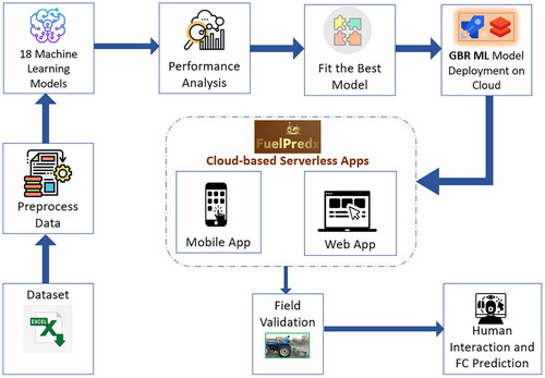
The fuel consumption model serves as a valuable tool for estimating real-time fuel consumption levels. An accurate fuel consumption model is crucial in providing precise information regarding fuel utilisation and motivating experts to assess the vehicle’s economy. The goal of this study was to develop a novel approach by eliminating the measurement of real-time tractor PTO (power take-off) power for fuel consumption prediction and to develop a cloud-infused, server-less, machine learning (ML) based real-time generalised tractor fuel consumption prediction model for any tractor between the power range of 8–48 hp. The fuel consumption prediction models from 18 Machine Learning algorithms were developed, and the extensive data analysis with hyperparameter tuning concluded that the Gradient Boosting Regressor Machine Learning model outperformed the other Machine Learning models with reasonable accuracy (R² = 0.999 for training and 0.914 for testing). Cloud-based serverless Web App and Android App integrated with the Gradient Boosting Regressor based fuel consumption prediction model were developed for the real-time fuel consumption prediction and monitoring of a tractor during field operations. The developed Machine Learning model predicted fuel consumption with a Mean Absolute Percentage Error of 11.43% during real-time field experiments with Mouldboard plough operation. The field validation showed the generalisation ability and efficacy of the developed model, and it can be implemented as a user advisory system for real-time energy-efficient agricultural operations.

Graphical Abstract

Keywords:

• Tractor fuel consumption prediction
• generalised model
• machine learning
• gradient boosting regressor
• cloud-driven serverless app
• android app

Reviewing Editor:

• Pham D T, University of Birmingham, UK

SUBJECTS:

• Agriculture & Environmental Sciences, Artificial Intelligence, Computation, Information & Communication Technology (ICT), Power & Energy, Technology

1. Introduction

Fuel is the primary energy source for a wide range of agricultural machinery and equipment, mainly for tractors to generate the necessary power to accomplish various agricultural activities. On the other hand, the percentage of fuel and lubricant costs range from a minimum of 16 per cent to over 45 per cent of the total machine costs and can vary depending on factors such as the type of fuel used and the duration of tractor or machine usage (Siemens & Bowers, 1999). Knowing the necessary details about tractor fuel consumption in developing nations helps manage fuel resources and production costs in a way that considers the rising trend in fuel prices. Furthermore, the agricultural sector’s annual diesel consumption rates have increased rapidly with a direct impact of the farm power availability, which has risen from 0.36 kW/ha in 1975–76 to about 2.76 kW/ha in 2021–22 and needs to be increased to 4.0 kW/ha by the end of 2030 (Singh & Singh, 2021). Regarding the farm power source, fuel consumption is one of the most important tractor performance parameters during any field operation. Engine size and load depend on the type of operating implement, such as plough, cultivator, harrow or rotary tiller, and operating depth and width, speed, and soil parameters like type, bulk density, and cone-index.

The ability to forecast tractor fuel consumption during field operations has been of great interest to manufacturers and scientists in order to optimise the field performance (Abdulrahman et al., 2010). To obtain this accurate information about fuel utilisation, the fuel consumption model is a valuable resource for experts, allowing for a precise assessment of the vehicle’s economy. In recent years, researchers have focused on studying the relationship and impact of engine operating parameters on the prediction of tractor fuel consumption using some mathematical models. These models can represent fuel consumption for specific tractor engine types as a function of operating engine speed and engine speed depression (difference between the operating engine speed and the engine speed at no load) at different throttle settings (Harris & Pearce, 1990). Furthermore, the model for fuel consumption prediction was formulated from laboratory experiments based on the equivalent tractor PTO power of the tractors included in the Nebraska test lab (Agricultural & Engineers, 2011; Grisso et al., 2006; Kheiralla et al., 2004; Kim et al., 2010; Kim et al., 2011; Rahimi-Ajdadi & Abbaspour-Gilandeh, 2011). However, researchers have paid particular attention to investigating and modelling the impact of operational parameters on different tractor fuel efficiency parameters: temporal fuel consumption, fuel consumption per working hour, fuel consumption per tilled area and specific volumetric fuel consumption for different tillage operations such as ploughing, harrowing, rotary tilling and subsoiling in different soil conditions (Almaliki et al., 2016b; Karparvarfard & Rahmanian-Koushkaki, 2015; Kheiralla et al., 2004; Moitzi et al., 2014).

Furthermore, the range of options for predicting fuel consumption of different tractor-implement combinations during tillage has been expanded due to the constant improvement of soft computing models in engineering-based simulation practises. Researchers have shown much interest in machine learning and other soft computing scenarios (ANNs and ANFIS) in this context, especially in forecasting and developing different tractor fuel consumption models for both stationary and field operating conditions (Al-Janobi et al., 2020; Almaliki et al., 2016a; Gijare et al., 2024; Jalilnezhad et al., 2023; Nagar & Machavaram, 2022; Shafaei et al., 2018b; Sperandio et al., 2023). A neurocomputing-based simulation strategy was able to simulate the tractor fuel efficiency parameters at different ploughing depths of 10, 20 and 30 (cm) and forward speeds of 2, 4 and 6 (km/h) with reasonable accuracy (Shafaei et al., 2018a, 2018b, 2019).

Each of these mathematical and soft computing models has unique equations with model coefficients and parameters that must be created repeatedly and require extensive data collection and processing to predict tractor fuel efficiency parameters. The limitation inspired researchers to develop user-friendly software and multi-objective programs linked to the model in the database to predict fuel consumption. The graphical user interface can reveal field tractor energy use in real-time by integrating analytic tools with the cloud-based server. It generates performance reports and improves farmers’ and the custom hiring centre’s experience. The tractor field performance comparison between power ranges can help the farmer and machine owner make informed decisions about real-time monitoring of operating parameters and fuel consumption prediction.

A classic example of this is the developed Windows-based software using the Visual Basic language to calculate the tractor fuel consumption based on the ballast requirements of a tractor’s front and rear wheels (Pranav & Pandey, 2008). A simulation model that provides precise specific fuel consumption (SFC) was developed for a two-wheel drive tractor attached with a cultivator, mould board plough and disc harrow operating in different soil conditions (Kolator & Białobrzewski, 2011; Kumar et al., 2017; Kumar & Pandey, 2015). In the same way, there is a need to conduct vast and repetitive experiments for a specific tractor to prognosticate the real-time fuel consumption prediction considering both engine and field performance parameters. Existing fuel consumption models, which are designed to establish a connection between fuel consumption and vehicle attributes, often suffer from limited computational efficiency. Hence, there is a demand for a data-centric real-time tractor fuel consumption prediction model that can provide precise predictions, possesses broad applicability with different power ranges of the tractors, and features easily interpretable parameters with user-friendly access from anywhere.

However, no such study has been done on developing a universal fuel consumption model that could be used for any engine power range of tractors by using soft computing techniques, and also the demonstration of the same using any user interface-based guidance system for the tractor operator. Therefore, in the present study, an ML-based universal fuel consumption prediction model was developed to predict the fuel consumption of a tractor for a variety of tractor power ranges (8–48 hp), and a serverless cloud-connected Android App and Web App was coupled with the developed ML-based model for the real-time prediction and monitoring of the tractor fuel consumption that can guide the tractor operator directly or remotely for a fuel efficient field operation.

2. Materials and methods

2.1. Dataset collection

The CFMTTI, Budni, India has a long history of conducting field and tractor drawbar tests at different operating points with various implements and sharing information about corresponding power and fuel consumption. Following testing standards and encompassing the natural and high ambient conditions, the high-speed diesel oil supplied by M/s Indian Oil Corporation Limited has a density of 0.836 g/cc at 15° C is used. Tractor fuel consumption at any operating point can be expressed as a universal function of engine speed at zero torque and the engine speed depression (difference between the engine speed at no load and operating point) (Harris & Pearce, 1990). Taking this into account, a dataset of 257 samples with 4 features (fuel consumption with maximum PTO power, engine speed, and engine speed depression for both full throttle and part throttle conditions) from 23 tractor test reports in the power range of 8–48 hp was collected from the CFMTTI. These tractors were explicitly selected to cover a wide power range of diesel engine specifications (engine design, injection system and timing, engine rated power and speed, etc.) from 8 to 48 hp. The dataset comprises three independent parameters, viz, (i) tractor maximum PTO power, which represents any tractor (including a wide range of diesel engine specifications) for generalisation, (ii) engine operating speed and (iii) engine speed depression; these two parameters represent throttle setting and load conditions of a tractor; the dependent parameter of the dataset is the corresponding fuel consumption of a tractor. The description (minimum, maximum, mean and standard deviation of various parameters) of the dataset is given in Table 1, and a sample dataset from two different power ranges (17 hp and 33.25 hp) of tractors is shown in Table 2.

Table 1. Dataset description for generalised ML model development.

	Independent parameters			Dependent parameter
Index	Tractor Max. PTO power (hp)	Engine speed (rpm)	R (speed depression) (rpm)	Fuel consumption (L/h)
count	257	257	257	257
mean	30.76	2222.45	90.33	4.48
std	12	364.50	89.88	2.43
min	7.5	1500	0	0.61
25%	16.76	1999	25	2.47
50%	33.40	2200	66	3.97
75%	38.49	2369	124	6.27
max	48.27	3517	518	11.53

Table 2. Sample worksheet of collected data for two different tractors.

Tractor ID	Max. PTO power (hp)	Operating engine speed (rpm)	Throttle setting (%)	R (speed depression) (rpm)	Fuel consumption (L/h)
T 18	17	2003	100	142	3.75
T 18	17	2058	100	87	3.39
T 18	17	1500	50	356	2.90
T 18	17	1745	50	111	2.74
T MF 1035	33.25	2003	100	163	7.15
T MF 1035	33.25	2042	100	124	6.17
T MF 1035	33.25	1500	50	233	5.77
T MF 1035	33.25	1611	50	122	5.39

2.1.1. Data visualisation

The dataset was analysed using a machine learning tool called data visualisation that offers a graphical representation of the datasets, making it easier to comprehend the variation between the different variables. The Pearson correlation coefficient $r$ (Cohen et al., 2009) with their corresponding dataset distribution has been calculated using Equation (1)(1) $$r=\frac{\sum \left(X_i-\overline{X}\right)\left(Y_i-\overline{Y}\right)}{\sqrt{\sum {\left(X_i-\overline{X}\right)}^2{\left(Y_i-\overline{Y}\right)}^2}}$$(1) , which is shown in Figure 1. It can be observed from Figure 1 that fuel consumption FC (L/h) has a strong positive correlation with the tractor PTO power (hp) and engine speed depression (rpm), respectively, with $r=0.60\mathrm{ }$ and $r=0.57,$ and negative correlation with the operating engine speed (rpm) having $r=-0.28.$

Figure 1. Dataset correlation among different input and output variables.

(1) $$r=\frac{\sum \left(X_i-\overline{X}\right)\left(Y_i-\overline{Y}\right)}{\sqrt{\sum {\left(X_i-\overline{X}\right)}^2{\left(Y_i-\overline{Y}\right)}^2}}$$(1)

where $X_i$ and $Y_i$ are the individual data points of variables X and Y, respectively. $\overline{X}$ and $\overline{Y}$ are the means of variables X and Y, respectively, and the summation $(\Sigma )$ is taken over all data points (i = 1 to n)

2.1.2. Dataset preprocessing

The data pre-processing was performed for the given dataset using the PyCaret library (2022) version 3.4.0 (Ali, 2020) in Google Colab; it is essential before feeding the datasets into machine learning models to eliminate irrelevant noise, handle missing values, address outliers, perform label encoding, and other necessary tasks. The original size of the dataset is (257, 4), and after the preprocessing, the size of the transformed dataset is (248,4). A brief description of the dataset preprocessing using the PyCaret library is given in Table 3, and the transformed dataset after the preprocessing has been used for training, validation and testing of the machine learning models.

Table 3. The brief description of the dataset preprocessing using PyCaret library.

S. No	Description	Value
0	Original data shape	(257, 4)
1	Target	FC (L/h)
2	Numeric features	3
3	Session id	6830
4	Transformed data shape	(248, 4)
5	Transformed train set shape	(174, 4)
6	Transformed test set shape	(74, 4)
7	Target type	Regression
8	Preprocess	TRUE
9	Imputation type	simple
10	Numeric imputation	mean
11	Categorical imputation	mode
12	Remove multicollinearity	TRUE
13	Multicollinearity threshold	0.9
14	Remove outliers	TRUE
15	Outliers threshold	0.05
16	Transformation	TRUE
17	Transformation method	yeo-johnson
18	Normalise	TRUE
19	Normalise method	zscore
20	Transform target	TRUE
21	Transform target method	yeo-johnson
22	Fold generator	KFold
23	Fold number	10
24	CPU jobs	−1
25	Use GPU	FALSE
26	Log experiment	FALSE
27	Experiment name	reg-default-name
28	USI	98a1

2.2. ASAE model for fuel consumption prediction

In this research, the fuel consumption prediction model specified by the Nebraska Tractor Test for tractor performance under ASAE Standard D497.4 (Agricultural & Engineers, 2011) has been used to predict the fuel consumption for different power ranges of tractors.

The standard formula for calculating the average fuel consumption of a tractor operating under various load conditions is (2) $$\mathrm{Q}=(2.64\times \mathrm{X}+3.91–0.203\times \sqrt{738\times X+173 })\times \mathrm{X}\times P_R$$(2)

Here,

Q is fuel consumption at partial loads, L/h,

X is the ratio of equivalent PTO power to rated PTO power, decimal, and

P_R is rated PTO power, kW.

The equivalent PTO power for any operation in the above equation can be calculated by knowing the engine torque and speed.

The ASAE fuel consumption model (Equation (1)(1) $$r=\frac{\sum \left(X_i-\overline{X}\right)\left(Y_i-\overline{Y}\right)}{\sqrt{\sum {\left(X_i-\overline{X}\right)}^2{\left(Y_i-\overline{Y}\right)}^2}}$$(1) ) predicts the fuel consumption of any tractor for a given PTO power; however, it could not interpret the throttle setting of a tractor during the fuel consumption prediction. Therefore, other advanced models or ML techniques are the alternatives for developing a generalised fuel consumption model considering the throttle setting of a tractor engine.

2.3. Machine learning models for fuel consumption prediction

Various diesel engines from 8 to 75 hp are used in Indian tractors, and the tractor engine fuel consumption prediction is affected by the engine load (torque) and speed. In this study, an ML-based generalised fuel consumption prediction model was developed to predict the fuel requirements of all tractors in the power range under field operating conditions.

2.3.1. Machine learning (ML) model development

A total of 18 machine learning algorithms were selected to develop a generalised fuel consumption prediction model, and the collected dataset was used for the training, validation and testing of these models. The 18 ML PyCaret regressors with respective parameters and descriptions have been listed in Table 4.

Table 4. Brief description of the PyCaret regressors with their parameters used for the ML model development.

Acronym	Estimator	Description	Parameters
lr	Linear regression (Montgomery et al., 2021)	A method that uses a straight line to depict how one or more independent and dependent variables are related.	copy_X, fit_intercept, n_jobs, positive
ridge	Ridge regression (Rifkin & Lippert, 2007)	A method for building a model when there are more predictor variables than observations.	random_state, copy_X, fit_intercept, alpha, tol, max_iter, positive, solver
lasso	Lasso regression (Friedman et al., 2010)	A kind of linear regression that makes use of shrinkage when data values are shifted in the direction of a midpoint, like the mean.	precompute, alpha, selection, random_state, warm_start, copy_X, fit_intercept, max_iter, positive, tol
lar	Least angle regression (lar) (Efron et al., 2004)	A linear regression that chooses the model to address the overfitting issue.	copy_X, eps, fit_intercept, fit_path, jitter, n_nonzero_coefs, normalize, precompute, random_state, verbose
llar	Lasso Least angle regression (llar) (Efron et al., 2004)	A comprehensive framework that more effectively fit Lasso model in high-dimensional problems.	jitter, normalize, positive, precompute, max_iter, verbose, fit_intercept, alpha, copy_X, eps, fit_path, random_state
br	Bayesian ridge (br) (MacKay, 1992)	A probabilistic model used for regression problems.	compute_score, alpha_1, lambda_2, tol, lambda_1, alpha_2, verbose, alpha_init, copy_X, fit_intercept, lambda_init, n_iter
par	Passive aggressive regressor (par) (Crammer et al., 2006)	An online learning method for both regression and classification.	validation_fraction, tol, warm_start, n_iter_no_change, shuffle, random_state, C, average, max_iter, early_stopping, epsilon, loss fit_intercept, verbose
dummy	Dummy Regressor (dummy) (Hardy, 1993)	A simple baseline model used for comparison in regression tasks, where it predicts target values based on simple rules like mean, median, or constant values without considering any input features.	constant, quantile, strategy
	Elastic net (en) (Friedman et al., 2010)	A useful linear regression model with numerous correlated features and a high likelihood of selecting both.	max_iter, positive, precompute, random_state, tol, fit_intercept, l1_ratio, selection, copy_X, warm_start, alpha
huber	Huber regressor (huber) (Verducci et al., 2007)	A robust regression approach to outliers.	alpha, epsilon, fit_intercept, max_iter, tol, warm_start
rf	Random forest (rf) (Breiman, 2001)	An approach to ensemble learning for regression or classification.	ccp_alpha, bootstrap, criterion, max_depth, max_features, max_leaf_nodes, max_samples, min_impurity_decrease, min_samples_leaf, min_samples_split, min_weight_fraction_leaf, n_estimators, n_jobs, oob_score, random_state, verbose, warm_start
et	Extra trees regressor (et) (Geurts et al., 2006)	A tree regressor that is extremely random. It only appears in ensemble methods.	oob_score, random_state, bootstrap, min_samples_split, n_jobs, max_features, min_impurity_decrease, ccp_alpha, criterion, max_depth, max_leaf_nodes, max_samples, min_samples_leaf, min_weight_fraction_leaf, n_estimators, verbose, warm_start
gbr	Gradient boosting regressor (gbr) (Friedman, 2001)	Utilises the ensemble decision tree regressor model principle.	max_leaf_nodes, learning_rate, init, ccp_alpha, min_impurity_split, n_iter_no_change, power_transformer_method, power_transformer_standardize, max_features, regressor, alpha, criterion, loss, max_depth, min_samples_leaf, min_samples_split, min_weight_fraction_leaf, n_estimators, presort, random_state, subsample, tol, validation_fraction, verbose, warm_start, min_impurity_decrease
lightgbm	Light gradient boosting machine (lightgbm) (Ke et al., 2017)	A potent gradient boosting framework based on the decision tree algorithm for classification, regression, and other machine learning tasks.	random_state, boosting_type, class_weight, colsample_bytree, importance_type, learning_rate, max_depth, min_child_samples, min_child_weight, min_split_gain, n_estimators, n_jobs, num_leaves, objective, reg_alpha, reg_lambda, silent, subsample, subsample_for_bin, subsample_freq
omp	Orthogonal matching pursuit (omp) (Rubinstein et al., 2008)	A greedy compressed sensing recovery algorithm that chooses the sensing matrix’s best-fitting column for each iteration.	tol, normalise, fit_intercept, precompute, n_nonzero_coefs
knn	K neighbors regressor (knn) (Kramer & Kramer, 2013)	A straightforward algorithm to forecast the desired value using a similarity metric across all potential cases.	weights, n_neighbors, metric_params, algorithm, n_jobs, metric, p, leaf_size
dt	Decision tree (dt) (Breiman, 2001; Freund & Mason, 1999)	A nonparametric supervised learning technique that uses straightforward decision rules influenced by the characteristics of the data to build models that forecast the value of a target variable.	max_features, splitter, random_state, criterion, max_depth, min_samples_split, min_samples_leaf, min_weight_fraction_leaf, ccp_alpha, max_leaf_nodes, min_impurity_decrease
ada	AdaBoost regressor (ada) (Freund & Schapire, 1997)	A machine learning meta-algorithm that enhances performance when combined with various learning algorithms.	loss, learning_rate, base_estimator, n_estimators, random_state, estimator

The configuration of the computational power used for the model development is given in Table 5. A systematic selection, execution and evaluation of the18 ML algorithms one by one was performed using an algorithm as shown in Figure 2.

Figure 2. An algorithm for the development of ML-based fuel consumption prediction.

Table 5. Configuration of the computational power used for the ML-based model development.

Resource	Details
Processor	Intel® Core™ i-5-7200U CPU @ 2.71 GHz
RAM	8 GB
GPU	Intel® UHD Graphics
Experimental tool	Google Colab

2.3.2. Model performance indicators

The performance prediction of the developed ML model was assessed using various statistical indicators, including the root mean squared error (RMSE), mean absolute error (MAE), coefficient of determination (R²), root mean squared loss error (RMSLE), mean squared error (MSE), and mean absolute percentage error (MAPE). The expressions for the performance indicators are given below. High R² values and low MSE primarily determine the developed ML model’s predictive performance. (3) $$R^2=1-\frac{\mathit{\text{sum squared regression}}\left(\mathit{\text{SSR}}\right)}{\mathit{\text{Total sum of squares}}\left(\mathit{\text{SST}}\right)}$$(3) (4) $$\mathit{\text{MSE}}=\frac{1}{n}\sum _{i=1}^n{(y_i-{\widehat{y}}_i)}^2$$(4) (5) $$\mathit{\text{MAE}}=\frac{1}{n}\sum _{i=1}^n|y_i-{\widehat{y}}_i|$$(5) (6) $$\mathit{\text{RMSE}}=\sqrt{\sum _{i=1}^n\frac{{{(y}_i-{\widehat{y}}_i)}^2}{n}}$$(6) (7) $$\mathit{\text{RMSLE}}=\sqrt{\sum _{i=1}^n\frac{{{\left(\right(\mathrm{\text{log}}(y}_i+1)‐\mathrm{\text{log}}({\widehat{y}}_i-1\left)\right)}^2}{n}}$$(7) (8) $$\mathit{\text{MAPE}}=\frac{1}{n}\sum _{i=1}^n\frac{(y_i-{\widehat{y}}_i)}{y_i}\times 100$$(8) where SSR = Sum of squared regression also referred to as a model-explained variation; SST = sum of the squared total, another name for the data’s overall variation. $y_i$ = i^th actual value. ${\widehat{y}}_i$ = i^th predicted value. n = total observations.

2.3.3. Hyperparameter tuning

Hyperparameters are predefined parameters in machine learning algorithms that govern the models’ behaviour and are crucial to minimise errors within the model. To address this, the GridSearchCV method was employed in this study for hyperparameter tuning. The comparison of the performance indicators of all 18 ML algorithms before and after hyperparameter tuning with the best performance was recorded.

2.4. Cloud-based serverless user interface for real-time prediction

The serverless approach for both the Web App and Android App development was used in this study for real-time fuel consumption prediction. A serverless user interface, also known as serverless computing or function as a service (FaaS), is a cloud computing architecture where the cloud service provider handles the infrastructure management. Serverless web applications offer developers a way to build scalable, cost-efficient, and easily maintainable applications without server provisioning and management.

2.4.1. Web App development

The best-performing ML model of the 18 algorithms was trained and tested using Python PyCaret under Google Colab and then generated as a pickle file. The Streamlit application also created an API to connect the webpage to the machine learning model. The URL-hosted Web Application runs on stlite, a serverless streamlit platform, so no data is sent to external servers. All Web App development in this study occurs in a local browser environment, limiting hardware resource allocation and server redundancy.

2.4.2. Android App development

A cloud-based serverless Android application (Android App) was constructed using React Native (Eisenman, 2015), and the API created previously for the Web App development was utilised in the mobile application development with the same input parameters. The process flow diagram of execution of the developed Web App and Android App deployed with a cloud-coupled ML model for the real-time fuel consumption prediction is shown in Figure 3.

Figure 3. Process flow for the execution of Web App and Android App with the cloud-coupled ML model for real-time fuel consumption prediction.

2.5. Experimental validation

An experimental setup was developed for validating the ML-based generalised fuel consumption prediction model in the actual field conditions. The developed experimental setup was calibrated and installed on an MFWA tractor of 43 hp as a test tractor. A detailed description of each device of the experimental setup is discussed below.

2.5.1. Real-time engine operating speed measurement

The test tractor’s engine crankcase had an inductive proximity sensor (Model: Proximon S18NON) 8 mm from the crankshaft pulley. An iron M8 bolt was mounted on the engine crankshaft pulley, and the proximity sensor receives signals when the bolt approaches, measuring the engine’s speed in real-time. Figure 4 shows the engine speed experiment setup. An Amprobe TACH-10 non-contact tachometer validated proximity sensor-based engine speed measurements, with a standard deviation of ± 0.5 rpm.

Figure 4. Engine speed (rpm) measurement setup on the test tractor.

2.5.2. Fuel consumption measurement

Figure 5 shows the test tractor’s experimental setup for real-time fuel consumption measurement. Two fuel flow metres are on the engine’s main and return fuel flow lines. The engine’s instantaneous fuel consumption is the difference between both fuel flow metres. An experimental setup was calibrated for accuracy using a test tractor measuring cylinder and had a maximum error of 1.5% compared to manual measurements (Figure 6).

Figure 5. Developed fuel flow rate calibration setup for tractor.

Figure 6. Calibrated results of the fuel flow sensors at different throttle settings.

2.5.3. Embedded systems for real-time data collection

The embedded system for measuring the tractor operating parameters includes an amplifier to amplify data from the proximity and fuel flow sensors, and the amplified sensor outputs were connected to the microcontroller’s digital pins (2, 3, 4). The inner view of the embedded system for on-the-go data recording of tractor parameters and the circuit diagram of the developed embedded system are shown in Figure 7(a) and 7(b), respectively.

Figure 7. Electronic embedded system for the real-time measurement of engine speed and fuel flow rate.

The test tractor was operated in sandy clay loam soil attached with a two-bottom MB plough (Figure 8) in the research farm of the Agricultural and Food Engineering Department of IIT Kharagpur, located at 22° 18′ 52.36′′ N and 87° 18′ 32.64′′ E.

Figure 8. Field operation for data collection of NH 4710 test tractor attached with MB plough.

3. Results and discussion

3.1. Performance of machine learning models on fuel consumption prediction

In this section, a total of 18 classic machine learning models were assessed for fuel consumption prediction based on various performance metrics, including root mean squared error (RMSE), mean absolute percentage error (MAPE), mean squared error (MSE), mean absolute error (MAE), coefficient of determination (R²) and root mean squared logarithm error (RMSLE). While all these algorithms fall under ensemble learning and use decision trees as their base learners, they differ in how they build and combine these trees, the level of randomisation introduced, and their optimisation strategies.

The hyperparameter tuning was performed for all 18 ML models, and the efficacy of these models was assessed based on the performance indicators, as shown in Figure 9. It can be seen from Figure 9 that the Gradient Boosting Regressor (GBR) demonstrated the best performance during its training and testing phase compared to the other ML models. It could indicate that the boosting process effectively leverages the information in the training dataset. GBR typically includes an adaptive learning rate, allowing for slower learning in regions where the model is already performing well and faster learning in areas where improvements are needed. This can lead to faster convergence and better results. Moreover, it includes the regularisation techniques, such as shrinkage and tree depth limitations, which can make it more robust to overfitting compared to models like Random Forest, especially in situations where the dataset is not extremely large (Friedman, 2001; Moghadasi et al., 2021). GBR exhibited the superior performance for the test dataset with the lowest values of RMSE (0.2333) and MAPE (0.0741), as well as the highest R² (0.9144), followed by Extra Trees Regressor [RMSE (0.3125), MAPE (0.1154), and R² (0.8654)], Random Forest Regressor [RMSE (0.6254), MAPE (0.1548), and R² (0.8418)], and Light Gradient Boosting Machine [RMSE (0.9054), MAPE (0.1845), and R² (0.8018)].

Figure 9. Comparison of performance indicators (MAE, MSE, RMSE, R², RMSLE and MAPE) for all 18 ML algorithms before tuning and after tuning.

Therefore, the Gradient Boosting Regressor was selected for its superior performance in developing a generalised fuel consumption prediction model for a wide power range of tractors in any operational conditions.

3.2. Performance of gradient boosting regressor (GBR) on fuel consumption prediction

The Gradient Boosting Regressor (GBR) performed efficiently for the fuel consumption prediction of tractors in the 8–48 hp power range compared to other ML models before and after hyperparameter tuning. The converged training and cross-validation scores of GBR after hyperparameter tuning are 0.99 and 0.89, respectively (Figure 10) during its learning after 150 instances. The residual plot of GBR for fuel consumption prediction after hyperparameter tuning is shown in Figure 11. The feature importance map of the GBR ML model for the generalised fuel consumption prediction is shown in Figure 12. It is seen from the figure that the fuel consumption of a tractor mostly depends on engine speed depression due to the applied engine load followed by tractor maximum PTO power and engine operating speed; it is in line with the empirical formulation of fuel consumption prediction by Harris model (Harris & Pearce, 1990). The regression plot of the GBR ML model for the test dataset is shown in Figure 13; it is seen from the figure that the developed GBR ML model lies reasonably close to the parity line with a coefficient of determination (R²) of 0.914 for fuel consumption prediction for the test dataset. It demonstrates the model reliability that captures the underlying relationship between the predictors and the response variables.

Figure 10. Training and cross-validation score for gradient boosting regressor during its learning.

Figure 11. Residuals for gradient boosting regressor during training and testing for fuel consumption prediction.

Figure 12. Feature importance plot for fuel consumption prediction by gradient boosting regressor.

Figure 13. Fuel consumption prediction performance of gradient boosting regressor for test dataset.

3.3. Generalised GBR ML model performance on other tractors

The developed GBR ML model showed its generalisation ability for fuel consumption prediction of tractors in the 8–48 hp power range during its training and testing, as described in the previous section. Therefore, it can be applied as a generalised GBR ML model for the fuel consumption prediction on two other tractors with a maximum PTO power of 20 hp and 30 hp to validate its performance for its generalisation ability. The actual fuel consumption of the two other tractors and the predicted fuel consumption by the generalised GBR ML model are plotted and shown in Figures 14 and 15 for tractors with maximum PTO power of 20 hp and 30 hp, respectively. It is seen from Figures 14 and 15 that the predicted fuel consumption of a tractor engine increases with engine operating speed and engine speed depression. It is in line with the actual fuel consumption of a tractor and other literature (Agricultural & Engineers, 2011; Grisso et al., 2006; Harris & Pearce, 1990; Kim et al., 2010; Kim et al., 2011) because fuel consumption increases with engine operating speed due to the increased number of strokes of a fuel injection pump, and it also increases with engine speed depression due to load coming on to the engine. Hence, the developed model could rightly predict the behaviour of a tractor engine in any power range. It is also observed from Figures 14 and 15 that the actual fuel consumption readings at 50% and 100% throttle are falling in the same range of the predicted results by the GBR ML model of the 20 hp and 30 hp tractor with MAPE of 9.57% and 8.19% respectively.

Figure 14. FC (L/h) prediction by GBR ML model for a 20 hp tractor.

Figure 15. FC (L/h) prediction by GBR ML model for a 30 hp tractor.

3.4. Performance comparison between the existing and the developed GBR ML model

The developed GBR ML-based generalised model and existing ASAE standard fuel consumption prediction model described in section 2.2 were used for fuel consumption prediction of the test dataset consisting of 74 samples with their corresponding three inputs. The fuel consumption prediction by the ASAE model and the developed GBR ML model are compared with the actual fuel consumption of a test tractor; the fuel consumption prediction comparison is shown in Figure 16.

Figure 16. Comparison of the actual and predicted fuel consumption for the test dataset.

The box-plot comparison of MAPE during fuel consumption prediction of the testing dataset for both models has been shown in Figure 17. The analysis depicted in Figures 16 and 17 clearly indicates that the fuel consumption predicted by the ASAE model tends to overestimate the actual fuel consumption values with a MAPE of 35.76 ± 20.34%. This overestimation trend aligns with the findings of previous research (Karparvarfard & Rahmanian-Koushkaki, 2015; Kheiralla et al., 2004; Rahimi-Ajdadi & Abbaspour-Gilandeh, 2011). In this contrast, the GBR ML model that was developed in the present study exhibits remarkable accuracy with MAPE of 7.41 ± 4.95% in predicting the fuel consumption of the different tractors within the specified power range across different load and throttle settings.

Figure 17. Box-plot comparison of MAPE for ASAE and developed GBR ML model for fuel consumption prediction of the testing dataset.

Considering that the ASAE model was derived from laboratory operations of tractors during the Nebraska Tractor Test, where different power and fuel consumption settings were evaluated at the rated engine speed, it was anticipated to observe such significant disparities in overestimation, whereas, in the present study, the developed GBR ML based generalised fuel consumption model was formulated using the test reports published by the Central FMTTI Indian institute, which is based on the field operations and drawbar tests of different tractors in the power range of 8–48 hp in different engine operating conditions.

3.5. Serverless user interface for monitoring of real-time fuel consumption prediction

The real-time fuel consumption output predicted by using the Android app is depicted in Figure 18. The Android App (Figure 18) takes the input from the user for maximum PTO power, engine operating speed, and engine speed depression and displays the fuel consumption, which is predicted through the developed GBR Model.

Figure 18. Real-time fuel consumption prediction output on the developed Android App (FuelPredx).

3.6. Field experimental validation of the developed GBR ML model

The graphical representation of the predicted fuel consumption by the GBR ML-based generalised model in comparison with the actual fuel consumption of a test tractor (NH 4710) at different loads and throttle settings during field operation using a two-bottom MB Plough is shown in Figure 19. The box plot of MAPE for each throttle setting is also presented in Figure 20. The developed GBR ML-based generalised model predicted the fuel consumption of the NH 4710 tractor with a coefficient of determination (R²) of 0.897 and MAPE of 11.43%, compared to the actual fuel consumption during field experiments.

Figure 19. Fuel consumption of NH 4710 tractor at different throttle settings during field operation compared with the GBR ML Model fuel consumption prediction.

Figure 20. Boxplot of mean absolute percentage error (MAPE) for predicted fuel consumption of NH 4710 tractor at different throttle settings.

Therefore, the developed cloud-based serverless Web App and Android App integrated with the developed generalised fuel consumption model by GBR ML Model are effective tools for monitoring the real-time fuel consumption of any tractor taking maximum PTO power, engine operating speed and engine speed depression (due to load at a particular throttle setting) as inputs. The developed Apps can be used as a user guidance and advisory system for economic and energy-efficient field operations in real-time, and these Apps can be implemented in different tractor field operations of custom hiring centres and cooperative farming centres.

4. Conclusions

The specific conclusions of the present study are listed as follows:

1. The GBR ML model showed better performance among 18 selected ML models with a low mean squared error of 0.06 for both the training and testing data and a high coefficient of determination (R²) of 0.999 for the training data and 0.914 for the testing data.

2. Tractor engine fuel consumption was predicted using the ASAE and the developed GBR ML model for comparison study. The MAPE of the ASAE model is 35.76%, whereas it is 7.41% for the developed GBR ML for the test dataset.

3. A cloud-based serverless Web App and Android App integrated with the developed GBR ML-based fuel consumption prediction model were developed as user-friendly and cost-efficient tools, allowing convenient real-time access for users from anywhere to the fuel consumption of a tractor from the GBR ML model predictions.

4. Experimental field validation of a 43 hp tractor attached with MB plough ensured the accuracy of the developed GBR ML-based fuel consumption prediction with the coefficient of determination (R²) of 0.897 with MAPE = 11.49%.

While demonstrating high accuracy, the developed fuel consumption prediction model for tractors within the 8–48 hp power range presents some limitations. These include its specificity to the defined power range, potential challenges in generalising it to other agricultural power equipment and focusing only on fuel consumption prediction. Future research should extend the power range and other power sources, assessing the model’s robustness across diverse agricultural operations.

Authors’ contributions

Harsh Nagar: conceptualization, methodology, data curation, formal analysis, software, writing–original draft, writing–review & editing, validation. Rajendra Machavaram: conceptualization, methodology, writing–original draft, supervision. Ambuj: writing–review & editing, software. Peeyush Soni: formal analysis, supervision. Vijay Mahore: methodology, validation. Prakhar Patidar: formal analysis. All authors affirm their shared responsibility and commitment to be accountable for all facets of the research work.

Acknowledgements

The authors would acknowledge the sincere appreciation for the research facilities of ICAR Project – CRP on Engineering Interventions in Precision Farming and Micro Irrigation Systems (PF & MIS).

Data availability statement

The data that support the findings of this study are available from the corresponding author upon reasonable request

Disclosure statement

The authors declare that they have no known competing financial interests or personal relationships that could have appeared to influence the work reported in this paper.

Additional information

Notes on contributors

Harsh Nagar

Harsh Nagar, Ambuj, Vijay Mahore and Prakhar Patidar are research scholars at the Agricultural and Food Engineering Department, Indian Institute of Technology Kharagpur, West Bengal, India. Rajendra Machavaram and Peeyush Soni are Associate Professors at the Agricultural and Food Engineering Department, Indian Institute of Technology Kharagpur, West Bengal, India.

Rajendra Machavaram

Harsh Nagar, Ambuj, Vijay Mahore and Prakhar Patidar are research scholars at the Agricultural and Food Engineering Department, Indian Institute of Technology Kharagpur, West Bengal, India. Rajendra Machavaram and Peeyush Soni are Associate Professors at the Agricultural and Food Engineering Department, Indian Institute of Technology Kharagpur, West Bengal, India.

  Ambuj

Harsh Nagar, Ambuj, Vijay Mahore and Prakhar Patidar are research scholars at the Agricultural and Food Engineering Department, Indian Institute of Technology Kharagpur, West Bengal, India. Rajendra Machavaram and Peeyush Soni are Associate Professors at the Agricultural and Food Engineering Department, Indian Institute of Technology Kharagpur, West Bengal, India.

Peeyush Soni

Harsh Nagar, Ambuj, Vijay Mahore and Prakhar Patidar are research scholars at the Agricultural and Food Engineering Department, Indian Institute of Technology Kharagpur, West Bengal, India. Rajendra Machavaram and Peeyush Soni are Associate Professors at the Agricultural and Food Engineering Department, Indian Institute of Technology Kharagpur, West Bengal, India.

Vijay Mahore

Harsh Nagar, Ambuj, Vijay Mahore and Prakhar Patidar are research scholars at the Agricultural and Food Engineering Department, Indian Institute of Technology Kharagpur, West Bengal, India. Rajendra Machavaram and Peeyush Soni are Associate Professors at the Agricultural and Food Engineering Department, Indian Institute of Technology Kharagpur, West Bengal, India.

Prakhar Patidar

Harsh Nagar, Ambuj, Vijay Mahore and Prakhar Patidar are research scholars at the Agricultural and Food Engineering Department, Indian Institute of Technology Kharagpur, West Bengal, India. Rajendra Machavaram and Peeyush Soni are Associate Professors at the Agricultural and Food Engineering Department, Indian Institute of Technology Kharagpur, West Bengal, India.

References

- Abdulrahman, A.-J., Saad, A.-H., & Aboukarima, A. (2010). An excel spreadsheet to estimate performance parameters for chisel plow-tractor combination based on trained an artificial neural network. Bulletin of University of Agricultural Sciences and Veterinary Medicine Cluj-Napoca. Agriculture, 67(2). https://doi.org/10.15835/buasvmcn-agr:5173
- Agricultural, A. S. O., & Engineers, B. (2011). Agricultural machinery management data. American Society of Agricultural and Biological Engineers.
- Ali, M. (2020). PyCaret: An open source, low-code machine learning library in Python. PyCaret Version, 2.
- Al-Janobi, A., Al-Hamed, S., Aboukarima, A., & Almajhadi, Y. (2020). Modeling of draft and energy requirements of a moldboard plow using artificial neural networks based on two novel variables. Engenharia Agrícola, 40(3), 363–373. https://doi.org/10.1590/1809-4430-eng.agric.v40n3p363-373/2020
- Almaliki, S., Alimardani, R., & Omid, M. (2016a). Artificial neural network based modeling of tractor performance at different field conditions. Agricultural Engineering International: CIGR Journal, 18(4), 262–274.
- Almaliki, S., Alimardani, R., & Omid, M. (2016b). Fuel consumption models of MF285 tractor under various field conditions. Agricultural Engineering International: CIGR Journal, 18(3), 147–158.
- Breiman, L. (2001). Random forests. Machine Learning, 45(1), 5–32. https://doi.org/10.1023/A:1010933404324
- Cohen, I., Huang, Y., Chen, J., Benesty, J., Benesty, J., Chen, J., Huang, Y., & Cohen, I. (2009). Pearson correlation coefficient. Noise reduction in speech processing, 1–4.
- Crammer, K., Dekel, O., Keshet, J., Shalev-Shwartz, S., & Singer, Y. (2006). Online passive aggressive algorithms.
- Efron, B., Hastie, T., Johnstone, I., & Tibshirani, R. (2004). Least angle regression.
- Eisenman, B. (2015). Learning react native: Building native mobile apps with JavaScript. O'Reilly Media.
- Freund, Y., & Mason, L. (1999). The alternating decision tree learning algorithm. ICML.
- Freund, Y., & Schapire, R. E. (1997). A decision-theoretic generalisation of on-line learning and an application to boosting. Journal of Computer and System Sciences, 55(1), 119–139. https://doi.org/10.1006/jcss.1997.1504
- Friedman, J. H. (2001). Greedy function approximation: A gradient boosting machine. Annals of Statistics, 29, 1189–1232.
- Friedman, J., Hastie, T., & Tibshirani, R. (2010). Regularisation paths for generalised linear models via coordinate descent. Journal of Statistical Software, 33(1), 1. https://doi.org/10.18637/jss.v033.i01
- Geurts, P., Ernst, D., & Wehenkel, L. (2006). Extremely randomised trees. Machine Learning, 63(1), 3–42. https://doi.org/10.1007/s10994-006-6226-1
- Gijare, S., Karthick, K., Juttu, S., Thipse, S. S., Paulraj, L. S., Jaiganesh, B., & Sridharan, S. (2024). Duty cycle based fuel consumption calculation using simulation methodology for agricultural tractor (0148-7191).
- Grisso, R. D., Vaughan, D. H., & Roberson, G. T. (2006). Method for fuel prediction for specific tractor models [Paper presentation]. 2006 ASAE Annual Meeting.
- Hardy, M. A. (1993). Regression with dummy variables (Vol. 93). Sage.
- Harris, H., & Pearce, F. (1990). A universal mathematical model of diesel engine performance. Journal of Agricultural Engineering Research, 47, 165–176. https://doi.org/10.1016/0021-8634(90)80038-V
- Jalilnezhad, H., Abbaspour-Gilandeh, Y., Rasooli-Sharabiani, V., Mardani, A., Hernández-Hernández, J. L., Montero-Valverde, J. A., & Hernández-Hernández, M. (2023). Use of a convolutional neural network for predicting fuel consumption of an agricultural tractor. Resources, 12(4), 46. https://doi.org/10.3390/resources12040046
- Karparvarfard, S., & Rahmanian-Koushkaki, H. (2015). Development of a fuel consumption equation: Test case for a tractor chisel-ploughing in a clay loam soil. Biosystems Engineering, 130, 23–33. https://doi.org/10.1016/j.biosystemseng.2014.11.015
- Ke, G., Meng, Q., Finley, T., Wang, T., Chen, W., Ma, W., Ye, Q., & Liu, T.-Y. (2017). Lightgbm: A highly efficient gradient boosting decision tree. Advances in Neural Information Processing Systems, 30.
- Kheiralla, A. F., Yahya, A., Zohadie, M., & Ishak, W. (2004). Modelling of power and energy requirements for tillage implements operating in Serdang sandy clay loam, Malaysia. Soil and Tillage Research, 78(1), 21–34. https://doi.org/10.1016/j.still.2003.12.011
- Kim, S., Kim, K., & Kim, D. (2011). Prediction of fuel consumption of agricultural tractors. Applied Engineering in Agriculture, 27(5), 705–709.
- Kim, S.-C., Kim, K.-U., & Kim, D.-C. (2010). Modeling of fuel consumption rate for agricultural tractors. Journal of Biosystems Engineering, 35(1), 1–9. https://doi.org/10.5307/JBE.2010.35.1.001
- Kolator, B., & Białobrzewski, I. (2011). A simulation model of 2WD tractor performance. Computers and Electronics in Agriculture, 76(2), 231–239. https://doi.org/10.1016/j.compag.2011.02.002
- Kramer, O., & Kramer, O. (2013). K-nearest neighbors. Dimensionality reduction with unsupervised nearest neighbors, 13–23.
- Kumar, N., & Pandey, K. (2015). A visual basic program for predicting optimum gear and throttle position for best fuel economy for 32 kW tractor. Computers and Electronics in Agriculture, 119, 217–227. https://doi.org/10.1016/j.compag.2015.10.024
- Kumar, A. A., Tewari, V., Gupta, C., & Kumar, N. (2017). A visual basic program and instrumentation system for power and energy mapping of tractor implement. Engineering in Agriculture, Environment and Food, 10(2), 121–132. https://doi.org/10.1016/j.eaef.2016.12.003
- MacKay, D. J. (1992). Bayesian interpolation. Neural Computation, 4(3), 415–447. https://doi.org/10.1162/neco.1992.4.3.415
- Moghadasi, M., Ozgoli, H. A., & Farhani, F. (2021). Steam consumption prediction of a gas sweetening process with methyldiethanolamine solvent using machine learning approaches. International Journal of Energy Research, 45(1), 879–893. https://doi.org/10.1002/er.5979
- Moitzi, G., Wagentristl, H., Refenner, K., Weingartmann, H., Piringer, G., Boxberger, J., & Gronauer, A. (2014). Effects of working depth and wheel slip on fuel consumption of selected tillage implements. Agricultural Engineering International: CIGR Journal, 16(1), 182–190.
- Montgomery, D. C., Peck, E. A., & Vining, G. G. (2021). Introduction to linear regression analysis. John Wiley & Sons.
- Nagar, H., & Machavaram, R. (2022). Application of artificial intelligence for fuel consumption prediction of a tractor in different operating conditions [Paper presentation]. 2022 IEEE 7th International Conference for Convergence in Technology (I2CT). https://doi.org/10.1109/I2CT54291.2022.9824626
- Pranav, P., & Pandey, K. (2008). Computer simulation of ballast management for agricultural tractors. Journal of Terramechanics, 45(6), 185–192. https://doi.org/10.1016/j.jterra.2008.12.002
- Rahimi-Ajdadi, F., & Abbaspour-Gilandeh, Y. (2011). Artificial neural network and stepwise multiple range regression methods for prediction of tractor fuel consumption. Measurement, 44(10), 2104–2111. https://doi.org/10.1016/j.measurement.2011.08.006
- Rifkin, R. M., & Lippert, R. A. (2007). Notes on regularised least squares.
- Rubinstein, R., Zibulevsky, M., & Elad, M. (2008). Efficient implementation of the K-SVD algorithm using batch orthogonal matching pursuit.
- Shafaei, S., Loghavi, M., & Kamgar, S. (2018a). An extensive validation of computer simulation frameworks for neural prognostication of tractor tractive efficiency. Computers and Electronics in Agriculture, 155, 283–297. https://doi.org/10.1016/j.compag.2018.10.027
- Shafaei, S., Loghavi, M., & Kamgar, S. (2018b). On the neurocomputing based intelligent simulation of tractor fuel efficiency parameters. Information Processing in Agriculture, 5(2), 205–223. https://doi.org/10.1016/j.inpa.2018.02.003
- Shafaei, S., Loghavi, M., & Kamgar, S. (2019). Reliable execution of a robust soft computing workplace found on multiple neuro-fuzzy inference systems coupled with multiple nonlinear equations for exhaustive perception of tractor-implement performance in plowing process. Artificial Intelligence in Agriculture, 2, 38–84. https://doi.org/10.1016/j.aiia.2019.06.003
- Siemens, J. C., & Bowers, W. (1999). Machinery management: How to select machinery to fit the real needs of farm managers. John Deere Pub.
- Singh, S., & Singh, S. (2021). Farm power availability and its perspective in Indian agriculture. RASSA Journal of Science for Society, 3(2), 114–126.
- Sperandio, G., Ortenzi, L., Spinelli, R., Magagnotti, N., Figorilli, S., Acampora, A., & Costa, C. (2023). A multi-step modelling approach to evaluate the fuel consumption, emissions, and costs in forest operations. European Journal of Forest Research, 143, 233–247. https://doi.org/10.1007/s10342-023-01624-2
- Verducci, J. S., Shen, X., & Lafferty, J. (2007). Prediction and discovery: AMS-IMS-SIAM joint summer research conference, machine and statistical learning: Prediction and discovery, June 25–29, 2006, Snowbird, Utah (Vol. 443). American Mathematical Soc.