Feature extraction-based liver tumor classification using Machine Learning and Deep Learning methods of computed tomography images

Abstract

The liver is an important and multifunctional human organ. Early and accurate diagnosis of a liver tumor can save lives. Computed Tomography (CT) images provide comprehensive information for liver tumor diagnosis using feature extraction techniques. These extracted features help classify liver tumors using Machine Learning (ML) and Deep Learning (DL) methods. For this research, twelve 1hundred CT images were acquired from the Radiology Department of Nishter Medical University & Hospital. The noise was removed using Gabor Filter after converting CT images into grayscale. Image quality was enhanced by adopting Histogram Equalization (HE), and finally, the Image’s edges and boundaries were improved using a smoothening and sharpening algorithm. Preprocessed images were forwarded to extract six features: Histogram, Run-length, Co-occurrence, Autogressive, Gradient, and Wavelet Transform. A major focus of this research is to evaluate that ML methods produced good accuracy using already extracted features while DL Algorithms could not produce better results. Firstly, ML methods such as Decision Tree (DT), Random Forest (RF), Boost, and Support Vector Machine (SVM) are deployed using an already extracted feature list containing all six features. It was observed that DT, RF, Boost, and SVM produced 96.5%, 99.6%, 99.7%, and 98.0% classification accuracy. After that, DL Algorithms such as Neural Networks (NN), Long-Short Term Memory (LSTM), Bi-Directional Long Short Term Memory (Bi-LSTM), and Convolutional Neural Networks (CNN) were deployed. The results showed that NN, LSTM, Bi-LSTM, and CNN produced 50.0%, 53.0%, 54.0%, and 54.0% accuracy respectively. To validate the major focus of this research, finally, Pre-trained DL Algorithms such as Residual Network 50 (Resnet50), Visual Geometry Group 16 (VGG16) and LSTM + CNN were deployed. Results showed that Resnet50, VGG16, and LSTM + CNN attained 78.0%, 88.0%, and 97.0% accuracy respectively. Hence, ML methods performed better using already extracted features, while DL Algorithms could not produce promising results on these extracted features.

KEYWORD:

• CT images
• computer vision
• Deep Learning
• feature extraction
• liver tumor
• Machine Learning

Reviewing Editor:

• Jenhui Chen, Chang Gung University, Taiwan; Xiangxiang Zeng, Xiamen University, China

Subjects:

• Algorithms & Complexity
• Artificial Intelligence
• Computer Science (General)

1. Introduction

The liver is a large, granularly essential organ in the human body. The unusual lifestyle of humans caused different diseases. Because of these diseases, liver cancer has become the most prevalent cancer in many regions of the world (Tummala & Barpanda, 2022). Liver cancer and tumors are one of the leading causes of death among other diseases across the globe (Das et al., 2019). One of the key areas of research in clinical diagnostic systems is the prevention and treatment of liver cancer (Na et al., 2013). Fast and diagnosis might have prevented many of these deaths. When diagnosing a patient’s disease, the doctor must make a clinical decision quickly based on available clinical information (Yankovy, 2021). An accurate and quick diagnosis depends on the doctor’s experience and skill in analysis. Most doctors could not diagnose properly due to unidentified properties of the liver and tumors. These unspecified properties include liver and tumor size and shape and one of the most promising reasons for misdiagnosis is the quality of imaging modalities.

Various imaging modalities such as Magnetic Imaging Resonance (MRI), CT, Ultrasound, Mammography, Angiography, and X-Rays aroused by different doctors for the diagnosis of various diseases (Napte, 2021). Most commonly, CT is the most widely used imaging modality for the detection of liver tumors. Doctors prefer CT imaging due to its speed, high resolution, and accuracy (Li et al., 2015). Doctors mostly used manual or semi-automated methods to segment liver tumors. Segmentation is a very difficult task due to the variable size of liver tumors and their shape. Therefore, an automated process for the segmentation of liver tumors helps doctors with quick, accurate, and early diagnosis of liver tumors.

Most of the researchers adopted various methods such as Machine Learning (ML), Deep Learning (DL), Statistical, clustering, and fuzzy-based methods for the diagnosis of liver tumors (Napte, 2021). Deep Learning (DL) methods have become popular in the last decade due to their versatility, accuracy, and fast execution to segment liver tumors. One of the most difficult challenges in the medical imaging field is segmenting an organ and the possible lesions identified inside it (Shah et al., 2021). Extracting information from an image involves several steps, including identifying specific features, object and pattern recognition, classification, and segmentation. This can be considered the study of segmenting the image into several regions with similar features named Region of Interest (Sharma, 2019).

For this research, ROI-based segmentation was adopted. The main objective of this research is to find ML methods that performed outstanding using already extracted features while DL algorithms could not achieve promising results. The experiments deployed ML and DL on the six features already extracted. The experiment results showed that ML algorithms performed well using the extracted feature list. On the other hand, DL algorithms produced poor results. The experiments were extended to validate the statement mentioned above. For this purpose, pre-trained DL Algorithms are deployed without an extracted feature list. As we know, Pre-trained DL Algorithms take images directly as input and extract features using their layers. It was observed that pre-trained DL Algorithms performed with good accuracy. These results validate that ML performs better using an already extracted feature list while DL could not produce better accuracy.

Section 2 showed the research contributions of different researchers in the field of Medical Imaging. It conducted a literature survey of ML, DL, Feature Extraction, and other methods introduced to classify and segment liver tumors.

2. Literature review

Medical imaging is a very promising area of research. Since the introduction of the computer vision field, many researchers have had to work on different systems to diagnose liver tumor. Researchers adopted the latest Artificial Intelligence (AI) based tools, techniques, and algorithms such as ML, DL, Pre-trained DL models, image segmentation, and feature extraction techniques. This section depicts the overview of research work conducted by researchers in this area.

2.1. Machine Learning methods

Many researchers adopted ML methods for the identification of liver tumors. In 2020, the ML system was introduced using an SVM classifier to classify liver tumors. The system used a region growth approach for liver and tumor segmentation. The proposed system classifies tumors into malignant and benign classes (Devi & Seenivasagam, 2020). In 2019, the SVM classifier was adopted for liver tumor classification. Histogram Oriented Gradient (HOG) technique was deployed for feature extraction using CT images (Al Sadeque, 2019). In 2019, an ML-based liver classification model was proposed. Random Forest (RF) accurately classified tumors from CT images. The active contour approach is used for liver and tumor segmentation (Agita, 2019). In 2018, another classification model was deployed using an RF classifier. Gabor filter is used for pixel-level feature extraction of CT images (Ezzatollah Shrestha, 2018). In 2017, an SVM classifier was adopted to identify tumorous and non-tumorous images. Fast Fourier Transform (FFT) is used for feature extraction. The model produced good accuracy (Jabarulla & Lee, 2017). In 2015, an automated liver tumor segmentation model was proposed. The model used SVM classifiers using binary features (Rajagopal, 2015). In 2014, K-nearest Neighbor (KNN) and multi-SVM classifiers were used for liver tumor classification. Mult-SVM produced higher accuracy as compared to KNN (Sakr, 2014). A Bayesian model was proposed for liver tumor segmentation using CT images (Aldeek, 2014). In 2013, Multi-Instance Learning (MIL) based method was introduced for liver tumor segmentation. SVM classifier is used to classify between cancer and normal liver CT images. The proposed method improved Region of Interest (ROI) based segmentation and classification accuracy (Jiang et al., 2013). Another multi-ROI-based liver tumor classification model was introduced in 2013. SVM classifier deployed using ROI-based extracted features liver tumors. The proposed model showed average classification accuracy (Jeon et al., 2013). A Computer-Aided Design (CAD) system was proposed in 2013. ROI-based Texture features were extracted. Principal Component Analysis (PCA) is used to train SVM classifiers (Virmani et al., 2013). In 2012, three classifiers named: KNN, SVM, and Artificial Neural Network (ANN) were used to identify healthy and steatosis infected livers. Ten cross-validations were used for all three classifiers. SVM produced better accuracy than all other classifiers (Andrade et al., 2012).

2.2. Deep Learning methods

On the other hand, researchers deployed DL Algorithms for liver tumor identification. In 2020, Resnet pre-trained network was adopted using CT images of the LiTS dataset. The proposed model produced average accuracy of 79% for liver tumor segmentation (Hille, 2022). In 2021, a hierarchical CNN-based model was proposed to classify liver tumors into benign and malignant classes. The proposed model produced 73.4% accuracy (Zhou et al., 2021) Artificial Neural Network (ANN) based model was proposed in 2021. The proposed model used the Adaptive Watershed algorithm along with ROI-based segmentation. Grey-level co-occurrence matrix (GLCM) is used for feature extraction. The model produced promising results to classify tumors into benign and malignant classes (Hemalatha & Sundar, 2021). Another CNN-based liver tumor segmentation model was proposed. The Z-Score algorithm is used for preprocessing images. Encoding method adopted for feature extraction from CT images. The proposed model produced good results (Aghamohammadi et al., 2021). A deep learning-based U-Net model was deployed to classify liver tumors using CT images. GLCM, Wavelet, and Spectral features were extracted using CNN. The proposed model achieved 80% classification accuracy (Swaraj, 2021). In the same year, two U-Net models were adopted to segment liver tumors from CT images. The image contrast was improved using the windowing technique (Paulatto et al., 2020). Another DL-based liver classification model will be proposed in 2021—region Growth technique adopted for taking ROIs. Weiner Filtering Algorithm (WFA) is used for image enhancement. Texture features were extracted, and the proposed model achieved good accuracy (Randhawa et al., 2021). A deep learning-based collaborative model is proposed for liver tumor classification using CT images in 2021. A modified U-Net model was adopted, and spatial features were extracted using Atrous Spatial Pyramid Pooling (ASPP) layer. The proposed model produced better accuracy (Gao & Almekkawy, 2021). In 2020, a fully convolutional network (FCN) was deployed to refine segmentation, and two convolutional neural networks were used to segment the liver. Fuzzy c-mean clustering was used for liver tumor identification (Zhang, 2020). A deep learning-based liver classification model was proposed in 2020. Signet network was adopted to extract the liver while UNet was used to extract the liver tumor. A hybrid algorithm named LeNet-ABC is used to extract and classify features from the liver tumor (Ghoniem, 2020). A neural network-based model was proposed in 2020 to identify tumors from CT images. Images were enhanced using Histogram Equalization and Median filters. Alexnet and Resnet were used for feature extraction. Finally, features were utilized for pixel-based classification (Elmenabawy, 2020).

The focus of the research is to evaluate that ML methods performed well and achieved higher accuracy using already extracted features, while DL Algorithms produced poor results on the extracted features. Pre-trained DL Algorithms were deployed for validation, which takes images as input instead of a features list. Section 3 comprises all experiments related to the main focus of the research.

3. Materials and methods

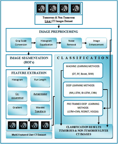
As mentioned above, the focus of the study is to evaluate ML, DL, and Pre-trained DL algorithms for accurate liver tumor detection using CT images. We proposed a model to uniquely identify liver tumors from the tumorous and non-tumorous classes of the CT images dataset. Firstly, CT images were preprocessed. Secondly, Histogram, Run-length, Co-occurrence, Autogressive, Gradient, and Wavelet Transform features were extracted. Thirdly, these features were optimized, and Finally, ML, DL, and Pre-trained DL algorithms were deployed to evaluate the performance for better accuracy. Expert radiologists and doctors manually examined the CT images to validate the ground truth of the dataset.

The proposed Enhanced Multi-Class Liver Tumor Identification (EMLTI) model is described in Figure 3.

2.1. Proposed methodology

The proposed EMLTI algorithm is described as follows:

2.2. Data acquisition

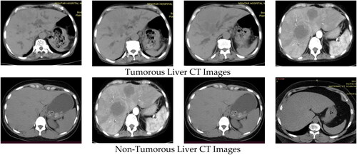
The major task of EMLTI is the collection of the CT image dataset. The two classes of the dataset are non-tumorous images and tumorous images, which include both benign and malignant types of images. The CT scans of one hundred twenty patients were selected for the research. Ten scans of the CT images of sixty patients were classified as tumorous, while the remaining sixty patients’ CT images were classified as non-tumorous. All images are (512 512) in size. Thus, in order to achieve high-quality results, the dataset comprises (120 × 10 = 1200 images) that have been converted into a BMP format. The images were collected from the Radiology Department of Nishter Medical University and Hospital, Multan, Pakistan (https://nmu.edu.pk). The CT images were captured using a Toshiba Aquilion Prime TSX-303A CT scanner with a resolution of 0.39–0.45 mm. The experienced radiologist examined the whole dataset manually. All the experimental results were shared with them. The Radiology Department of Nishter Medical University and Hospital, Multan, Pakistan, verified all the results. The dataset contains liver tumorous and non-tumorous CT images shown in Figure 1.

Figure 1. Tumorous and non-tumorous liver CT images dataset.

2.3. Image preprocessing

The next step after data acquisition is preprocessing. It involves several early stages of image analysis. The major objective of preprocessing is to improve the visual appearance of an image and enhance the image features for further processing (Hemalatha, 2016). Firstly, CT images were converted into a grey scale. Grayscale images are simpler for representation and have less computational requirements than color images (Hussain et al., 2022; Kanan & Cottrell, 2012). Grayscale conversions simplify further processing of an image due to its one-dimensional representation compared to the three-dimensional representation of a color image (Pound et al., 2014). Equation (1)(1) $$\mathrm{\text{Image}}=\frac{\mathrm{\text{Red}}+\mathrm{\text{Green}}+\mathrm{\text{Blue}}}{3}$$(1) depicts the grayscale conversion. 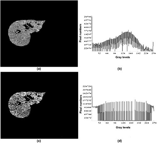(1) $$\mathrm{\text{Image}}=\frac{\mathrm{\text{Red}}+\mathrm{\text{Green}}+\mathrm{\text{Blue}}}{3}$$(1) where the variable Image comprises a grayscale image produced by calculating the mean of the values of the variables Red, Green, and Blue, which contains the values of the Red, Green, and Blue channels of the color image (Dwipayana, 2018). Converting CT images to Grey Scale employs a well-known technique known as windowing, which use a window width (WW) and window level (WL) to define a specific intensity range inside the Hounsfield Unit (HU) scale. Following that, normalization is performed to scale pixel values for analysis and display within a specific range, which is typically [0, 255] (Jung, 2021; Razi, 2014). Furthermore, Histogram Equalization (HE) was deployed to enhance the Image and its contrast. HE is a nonlinear stretch that redistributes pixel values so that there is approximately the same number of pixels with each value within a range (Hemalatha, 2016). The main idea behind HE is that each grey level occurs with the same frequency, resulting in an evenly distributed probability distribution and a flat histogram (Xiong et al., 2021). This will finally increase the contrast of an image as illustrated in Figure 2. All imaging techniques in radiology that use photons generate some noise due to the random distribution of photons. The CT image noise, on the other hand, can be calculated by comparing the level of desired photons to the level of background noise (Manson, 2019). After that, the noise was removed from the Image using Gabor Filter. The Gabor Filter is a Linear filter that, due to its low level pixel-by-pixel processing, can differentiate tumor mammography more accurately and simply (Bourkache, 2020; Dakshayani et al., 2022). A Gabor is a Gaussian Filter modulated with a function that is the product of Gaussian and Exponential Value, which is extensively used for image filtering (Dakshayani et al., 2022; Hussain et al., 2022). Finally, Spatial and Frequency domain filters are deployed for sharpening and smoothing images. Sharpening refers to enhancing the intensity of the image while smoothing refers to reducing blurring. Spatial linear filter was adopted for sharpening of images while and Gaussian low and high pass filters were smoothing of images in frequency domain (Fang et al., 2008).

Figure 2. Histogram Equalization (a) Liver image before HE. (b) Pre HE graph, (c) Liver image after HE, (d) Post HE graph (Ciecholewski, 2007).

2.4. Feature extraction

After Image preprocessing, CT images were segmented for tumor identification. Five Non-overlapping Region of Interest (ROI) were created manually to extract features. For this purpose, Ten Histogram, Twenty Run-Length, Twenty Co-occurrence, Ten Autogressive, Five Gradient, and Five Wavelet Transform features extracted from each ROI using Mazda software version 4.6. The total Feature Vector Table (FVT) for each ROI was 360,000(1200 x 60 x 5). These features in single or multiple combinations were adopted by different researchers using liver tumor images in different years (Hasan et al., 2023; Hussain et al., 2022; Krishan & Mittal, 2021; Moghimhanjani, 2022; Naeem et al., 2020). In this research, we adopted all these features collectively to produce better results.

2.4.1. Histogram features

Mean describes the central tendency of the histogram as shown in Eq. (2)(2) $$\mathrm{M}=\frac{1}{\mathrm{N}}\mathrm{ }\sum _{\mathrm{i}=1}^{\mathrm{N}}\mathrm{\text{Xi}}$$(2) . Variance describes how far the value lies from the mean, as shown in Eq. (3)(3) $${\mathrm{\mu }}^2=\frac{1}{\mathrm{M}}\mathrm{ }\sum _{\mathrm{i}=1}^{\mathrm{M}}{\left(\mathrm{\text{Yi}}-\stackrel{⃛}{\mathrm{Y}}\right)}^2$$(3) . Skewness measures the degree of asymmetry established by the data, as shown in Eq. (4)(4) $${\mathrm{\sigma }}_1=\frac{1}{\mathrm{T}}\mathrm{ }\sum _{\mathrm{i}=1}^{\mathrm{T}}{\left[\frac{\mathrm{\text{Zi}}-\stackrel{⃛}{\mathrm{\mu }}}{\mathrm{\phi }}\right]}^3$$(4) . If skewness equals zero, the histogram is symmetric about the mean. Kurtosis measures the peak of the histogram, as shown in Eq. (5)(5) $${\mathrm{\sigma }}_2=\frac{1}{\mathrm{T}}\mathrm{ }\sum _{\mathrm{i}=1}^{\mathrm{T}}{\left[\frac{\mathrm{\text{Zi}}-\stackrel{⃛}{\mathrm{\mu }}}{\mathrm{\phi }}\right]}^4-3$$(5) . The Kurtosis of a normal distribution is Zero.

Furthermore, Percentile refers to a specific position within a frequency distribution. It provides the baseline at which a desired proportion of scores lies—1, 10, 50, 90, and 99 percentile calculated for this research. The Percentile is shown in Eq. (6)(6) $$\mathrm{P}=\left(\frac{\text{Total Frequency}}{\mathrm{\text{Number}}}\right)\text{x}100$$(6) . (2) $$\mathrm{M}=\frac{1}{\mathrm{N}}\mathrm{ }\sum _{\mathrm{i}=1}^{\mathrm{N}}\mathrm{\text{Xi}}$$(2) (3) $${\mathrm{\mu }}^2=\frac{1}{\mathrm{M}}\mathrm{ }\sum _{\mathrm{i}=1}^{\mathrm{M}}{\left(\mathrm{\text{Yi}}-\stackrel{⃛}{\mathrm{Y}}\right)}^2$$(3) (4) $${\mathrm{\sigma }}_1=\frac{1}{\mathrm{T}}\mathrm{ }\sum _{\mathrm{i}=1}^{\mathrm{T}}{\left[\frac{\mathrm{\text{Zi}}-\stackrel{⃛}{\mathrm{\mu }}}{\mathrm{\phi }}\right]}^3$$(4) (5) $${\mathrm{\sigma }}_2=\frac{1}{\mathrm{T}}\mathrm{ }\sum _{\mathrm{i}=1}^{\mathrm{T}}{\left[\frac{\mathrm{\text{Zi}}-\stackrel{⃛}{\mathrm{\mu }}}{\mathrm{\phi }}\right]}^4-3$$(5) (6) $$\mathrm{P}=\left(\frac{\text{Total Frequency}}{\mathrm{\text{Number}}}\right)\text{x}100$$(6)

2.4.2. Run-Length features

Run Length features quantify gray-level runs in an image. A gray level is defined as the length of the number of pixels, of consecutive pixels with the same gray level value. Run Length Non-uniformity is shown in Eq. (7)(7) $$\mathrm{\text{RNNU}}=\sum _{\mathrm{j}=1}^{{\mathrm{m}}_{\mathrm{t}}}{\mathrm{L}}_{{\mathrm{t}}^2}$$(7) where ${\mathrm{L}}_{\mathrm{t}}$ denotes the sum of the distribution of the number of runs with run-length j and ${\mathrm{m}}_{\mathrm{t}}$ denotes the maximum run length. Similarly, Grey Level Non-uniformity, as shown in Eq. (8)(8) $$\mathrm{\text{GLNU}}=\sum _{\mathrm{i}=1}^{{\mathrm{L}}_{\mathrm{k}}}{\mathrm{Q}}_{{\mathrm{k}}^2}$$(8) where ${\mathrm{Q}}_{\mathrm{k}}$ denotes the sum distribution of the number of runs with run length, whereas ${\mathrm{L}}_{\mathrm{k}}$ denotes the number of discrete intensity values in the Image. Furthermore, Long run emphasis is depicted in Eq. (9)(9) $$\mathrm{\text{LHRE}}=\sum _{\mathrm{j}=1}^{{\mathrm{M}}_{\mathrm{r}}}\mathrm{ }{\mathrm{k}}^2{\mathrm{T}}_{\mathrm{r}}$$(9) , and Short-run emphasis in Eq. (10)(10) $$\mathrm{\text{SHRE}}=\sum _{\mathrm{j}=1}^{{\mathrm{M}}_{\mathrm{r}}}\frac{{\mathrm{T}}_{\mathrm{r}}}{{\mathrm{k}}^2}$$(10) . In both equations, ${\mathrm{T}}_{\mathrm{r}}$ denotes the sum of the distribution of the number of runs with run-length j and ${\mathrm{M}}_{\mathrm{r}}$ Showed the maximum run length. The fraction of Image in runs is shown in Eq. (11)(11) $$\mathrm{\text{RNP}}=\frac{{\mathrm{M}}_{\mathrm{z}}}{{\mathrm{M}}_{\mathrm{p}}}$$(11) where ${\mathrm{M}}_{\mathrm{z}}$ denotes the maximum run length and ${\mathrm{M}}_{\mathrm{p}}$ Showed the number of voxels in the Image. (7) $$\mathrm{\text{RNNU}}=\sum _{\mathrm{j}=1}^{{\mathrm{m}}_{\mathrm{t}}}{\mathrm{L}}_{{\mathrm{t}}^2}$$(7) (8) $$\mathrm{\text{GLNU}}=\sum _{\mathrm{i}=1}^{{\mathrm{L}}_{\mathrm{k}}}{\mathrm{Q}}_{{\mathrm{k}}^2}$$(8) (9) $$\mathrm{\text{LHRE}}=\sum _{\mathrm{j}=1}^{{\mathrm{M}}_{\mathrm{r}}}\mathrm{ }{\mathrm{k}}^2{\mathrm{T}}_{\mathrm{r}}$$(9) (10) $$\mathrm{\text{SHRE}}=\sum _{\mathrm{j}=1}^{{\mathrm{M}}_{\mathrm{r}}}\frac{{\mathrm{T}}_{\mathrm{r}}}{{\mathrm{k}}^2}$$(10) (11) $$\mathrm{\text{RNP}}=\frac{{\mathrm{M}}_{\mathrm{z}}}{{\mathrm{M}}_{\mathrm{p}}}$$(11)

2.4.3. Co-Occurrence features

The co-occurrence features define the occurrence probability of gray level with neighboring gray level. The angular second moment showed in Eq. (12)(12) $$\mathrm{\text{ASM}}={\sum }_{\mathrm{k}}{\sum }_{\mathrm{m}}{\left(\mathrm{N}(\mathrm{k},\mathrm{m})\right)}^2$$(12) , where k and m are the coordinates of the Co-occurrence matrix. Furthermore, Contrast and Correlation are shown in Eqs. (13)(13) $$\mathrm{\text{Contrast}}=\sum _{\mathrm{K}=1}^{{\mathrm{P}}_{\mathrm{g}}}\sum _{\mathrm{m}=1}^{{\mathrm{P}}_{\mathrm{g}}}{\left[\mathrm{N}(\mathrm{k},\mathrm{m})\right]}^2$$(13) and (14)(14) $$\mathrm{\text{Correlation}}=\frac{\sum _{\mathrm{K}=1}^{{\mathrm{P}}_{\mathrm{g}}}\sum _{\mathrm{m}=1}^{{\mathrm{P}}_{\mathrm{g}}}\mathrm{\text{kmN}}\left(\mathrm{k},\mathrm{m}\right)-{\mathrm{\mu }}_{\mathrm{x}}{\mathrm{\mu }}_{\mathrm{y}}}{{\mathrm{\sigma }}_{\mathrm{x}}{\mathrm{\sigma }}_{\mathrm{y}}}$$(14) , respectively where ${\mathrm{\mu }}_{\mathrm{x}}\text{and}{\mathrm{\mu }}_{\mathrm{y}}$ Is the mean of Nx and Ny. (12) $$\mathrm{\text{ASM}}={\sum }_{\mathrm{k}}{\sum }_{\mathrm{m}}{\left(\mathrm{N}(\mathrm{k},\mathrm{m})\right)}^2$$(12) (13) $$\mathrm{\text{Contrast}}=\sum _{\mathrm{K}=1}^{{\mathrm{P}}_{\mathrm{g}}}\sum _{\mathrm{m}=1}^{{\mathrm{P}}_{\mathrm{g}}}{\left[\mathrm{N}(\mathrm{k},\mathrm{m})\right]}^2$$(13) (14) $$\mathrm{\text{Correlation}}=\frac{\sum _{\mathrm{K}=1}^{{\mathrm{P}}_{\mathrm{g}}}\sum _{\mathrm{m}=1}^{{\mathrm{P}}_{\mathrm{g}}}\mathrm{\text{kmN}}\left(\mathrm{k},\mathrm{m}\right)-{\mathrm{\mu }}_{\mathrm{x}}{\mathrm{\mu }}_{\mathrm{y}}}{{\mathrm{\sigma }}_{\mathrm{x}}{\mathrm{\sigma }}_{\mathrm{y}}}$$(14)

2.4.4. Autogressive features

Autogressive features predict future values from past values, as shown in Eq. (15)(15) $$\mathrm{T}\left(\mathrm{s}\right)=\sum _{\mathrm{R}\in \mathrm{N}}{\mathrm{\theta }}_{\mathrm{R}}\mathrm{ }\mathrm{T}\left(\mathrm{s}+\mathrm{R}\right)+\mathrm{ }\sqrt{\mathrm{T}}\mathrm{ }\mathrm{X}\left(\mathrm{s}\right)\text{for s}\in \Omega$$(15) . Mazda provides five different features based on autoregressive model. These are theta 1 (parameter), theta 2 (parameter), theta 3 (parameter), theta 4 (parameter), and sigma (parameter). (15) $$\mathrm{T}\left(\mathrm{s}\right)=\sum _{\mathrm{R}\in \mathrm{N}}{\mathrm{\theta }}_{\mathrm{R}}\mathrm{ }\mathrm{T}\left(\mathrm{s}+\mathrm{R}\right)+\mathrm{ }\sqrt{\mathrm{T}}\mathrm{ }\mathrm{X}\left(\mathrm{s}\right)\text{for s}\in \Omega$$(15)

Where T(s) is the intensity of an image pixel at a location s = (x,y) and $\mathrm{\theta }$ (a,b) is the weighting coefficient N is the neighboring region, and Ω is the M x M lattice

2.4.5. Gradient features

Image gradient features measure the change of intensity in a specific direction. The gradient of the Image is the derivative of x and y in the two-dimensional function f(x,y). Gradient Mean, Gradient Variance, Gradient Skewness, and Gradient Kurtosis were observed for this research. The Gradient features computation shown in Eqs. (16)(16) $${\mathrm{G}}_{\mathrm{X}}\left(\mathrm{a},\mathrm{b}\right)=\mathrm{\text{Img}}\left(\mathrm{a}+1,\mathrm{b}\right)-1\left(\mathrm{a}-1,\mathrm{b}\right)$$(16) and (17)(17) $${\mathrm{G}}_{\mathrm{Y}}\left(\mathrm{a},\mathrm{b}\right)=\mathrm{\text{Img}}\left(\mathrm{a},\mathrm{b}+1\right)-1(\mathrm{a},\mathrm{b}-1)$$(17) . (16) $${\mathrm{G}}_{\mathrm{X}}\left(\mathrm{a},\mathrm{b}\right)=\mathrm{\text{Img}}\left(\mathrm{a}+1,\mathrm{b}\right)-1\left(\mathrm{a}-1,\mathrm{b}\right)$$(16) (17) $${\mathrm{G}}_{\mathrm{Y}}\left(\mathrm{a},\mathrm{b}\right)=\mathrm{\text{Img}}\left(\mathrm{a},\mathrm{b}+1\right)-1(\mathrm{a},\mathrm{b}-1)$$(17)

2.4.6. Wavelet transform features

Wavelet transform features enable the decomposition of an image for analysis, as shown in Eq. (18)(18) $$\mathrm{\text{WaveF}}\left(\mathrm{X},\mathrm{Y}\right)={\int }_{-\mathrm{\infty }}^{+\mathrm{\infty }}\mathrm{f}\left(\mathrm{a}\right)\frac{1}{{\mathrm{T}}^{\frac{\mathrm{M}}{2}}}\mathrm{ }{\mathrm{\mu }}^{\mathrm{*}}\left(\frac{\mathrm{a}-\mathrm{X}}{\mathrm{Y}}\right)\mathrm{d}\mathrm{x}$$(18) . A wavelet represents a particular location of something in an image. In wavelet transformation, the pixel vector of an image can be divided into different frequency components for further processing. The wavelet energy feature was observed for this research. (18) $$\mathrm{\text{WaveF}}\left(\mathrm{X},\mathrm{Y}\right)={\int }_{-\mathrm{\infty }}^{+\mathrm{\infty }}\mathrm{f}\left(\mathrm{a}\right)\frac{1}{{\mathrm{T}}^{\frac{\mathrm{M}}{2}}}\mathrm{ }{\mathrm{\mu }}^{\mathrm{*}}\left(\frac{\mathrm{a}-\mathrm{X}}{\mathrm{Y}}\right)\mathrm{d}\mathrm{x}$$(18)

Multi-featured dataset for this research requires Histogram, Run-Length, Co-occurrence, Autogressive, Gradient, and Wavelet Transform features. The experiments were performed in two different ways. Firstly, a complete feature list comprising all six features deployed using ML, DL, and Pre-trained algorithms. Finally, a feature list of each feature is deployed separately using ML, DL, and Pre-trained algorithms. This helps to compare the performance of each ML, DL, and Pre-trained algorithm based on features collectively and separately.

2.5. Classification

Four ML classifiers deployed: DT, RF, Boost, and SVM. Similarly, DL classifiers NN, LSTM, Bi-LSTM, and CNN were also deployed. Finally, Pre-trained Algorithms, namely, LSTM + CNN, Resnt50, and VGG16 also deployed. As mentioned above, two types of experiments were deployed for this research. Firstly, experiment performed using ML and DL algorithms with complete and individual feature list of all six features. Secondly, experiment performed using pre-trained algorithms which takes images directly as input instead of already extracted features. During experiments, it was observed that ML classifiers performed outstandingly as compare to DL classifiers using complete feature list and individual feature list as well. While unfortunately, DL classifiers produced low frequency using already extracted features list with complete and individual feature list. ML classifier RF, Boost, SVM, and DT produced 99.6%,99.7%, 98.0%, and 96.5% accuracy respectively using a complete feature list of six features. On the other hand, DL classifiers, NN, LSTM, Bi-LSTM, and CNN produced 50.0%, 53.0%, 54.0%, and 54.0% accuracy, respectively, using a complete feature list of all features. In second experiment, pre-trained DL algorithms: LSTM + CNN (Naeem & Bin-Salem, 2021; Rayan et al., 2023), Resnet50, and VGG16 attained 97.0%, 78.0%, and 88.0% accuracy respectively. These pre-trained DL algorithms takes images directly as input and automatically extract features of images. The aim of this research is to proof that DL algorithms could not produce better using already extracted manual feature list while the rational of using pre-trained DL algorithms is to support the fact that using automatic feature extraction layers of pre-trained algorithms can produce better results (Figure 3).

Figure 3. EMLTI liver tumor classification framework.

As mentioned earlier, the feature list was extracted before deploying ML and DL classifiers. ML classifiers were used with Ten-fold cross validation. The number of layers, filter size, activation function, and learning rate are examples of hyperparameters that must be chosen carefully to ensure optimal performance of DL algorithms (Desta et al., 2022). DL algorithms deployed with one hidden layer and neurons between 10 and 100. Already extracted features were directly input to network with activation function Relu. Batch size used for experiments was 1000 features. When we deployed the DL algorithm with already extracted features, it produced poor accuracy. To prove this fact, pre-trained DL algorithms were deployed. The CT images are directly input to these pre-trained algorithms. These pre-trained algorithms produced promising results.

4. Results

This research contributes to using four ML classifiers such as RF, Boost, SVM, and DT, and four DL classifiers as CNN, LSTM, Bi-LSTM, and NN. Pre-trained Algorithms such as LSTM + CNN, Resnet50, and VGG16 were also deployed. Two kinds of feature lists were prepared. The first one is a complete feature list containing all six features: Histogram, Run-Length, Co-occurrence, Autogressive, Gradient, and Wavelet Transform features. An individual feature list of each feature is also used for experiments. The accuracy factor was observed critically among all other performance evaluation factors. These experiments were deployed to validate that ML classifiers produced good classification accuracy using an extracted feature list compared to DL classifiers. For this purpose, experiments extended with the deployment of pre-trained DL algorithms.

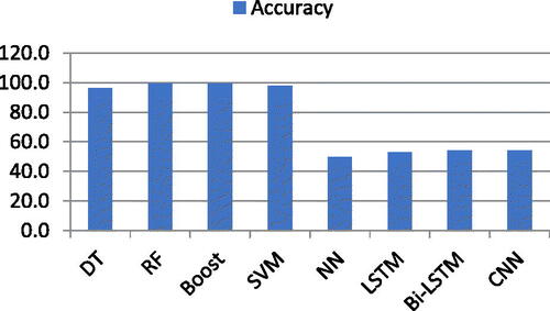
For this research, firstly, four ML classifiers such as RF, Boost, SVM, DT, and DL classifiers such as CNN, LSTM, Bi-LSTM, and NN, deployed on a feature list containing all six features extracted using ROI segmentation. The results showed that Boost produced 99.7% accuracy while RF, SVM, and DT produced 99.6%, 98.0%, and 96.5%, respectively. Tenfold cross validation was adopted. At the same time, CNN and Bi-LSTM produced 54.0% accuracy, respectively. On the other hand, NN and LSTM produced 50.0% and 53.0% accuracy, respectively. The accuracy factor was examined more closely than any other performance evaluation factors (Hussain et al., 2022). Those factors include F1-Scroe (Fs), Precision (Pn), Recall (Rc), False Positive (Fp), False Negative (Fn), True Positive (Tp), and True Negative (Tn) (Cavalin, 2019; Krstinic, 2020). According to multiple studies, the accuracy factor is the most important and often used performance evaluation metric (Hossin, 2015). Eq. (19)(19) $$\mathrm{\text{Accuracy}}=\frac{\mathrm{\text{Tp}}+\mathrm{\text{Tn}}}{\mathrm{\text{Tp}}+\mathrm{\text{Tn}}+\mathrm{\text{Fp}}+\mathrm{\text{Fn}}}\mathrm{ }$$(19) shows the calculation of Accuracy. (19) $$\mathrm{\text{Accuracy}}=\frac{\mathrm{\text{Tp}}+\mathrm{\text{Tn}}}{\mathrm{\text{Tp}}+\mathrm{\text{Tn}}+\mathrm{\text{Fp}}+\mathrm{\text{Fn}}}\mathrm{ }$$(19)

Where Tp, Tn, Fp and Fn represents True Positive, True Negative, False Positive and False Negative respectively.

The accuracy results of both ML and DL classifiers using the complete feature list of all six features are shown in Table 1.

Table 1. Accuracy of ML and DL classifiers using all features.

ML classifiers	Accuracy (%)	DL classifiers	Accuracy (%)
DT	96.5	NN	50.0
RF	99.6	LSTM	53.0
Boost	99.7	Bi-LSTM	54.0
SVM	98.0	CNN	54.0

The graphical representation of the accuracy obtained using ML and DL classifiers is shown in Figure 4.

Figure 4. Accuracy chart of ML and DL with complete feature list.

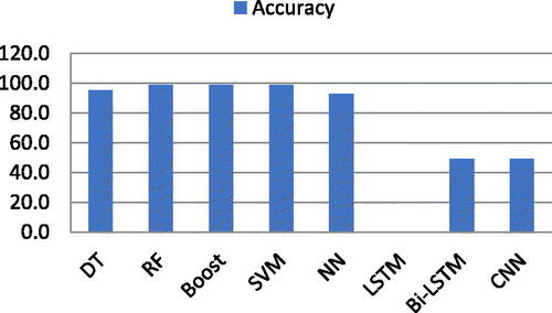
Now, the experiments are extended to a separate list of the six features mentioned above. Both ML and DL classifiers are deployed individually. Table 2 shows the accuracy of both ML and DL algorithms using features extracted using co-occurrence features. RF, Boost, and SVM produced 99.0% accuracy using the co-occurrence features list, while DT produced 95.0% accuracy. On the other hand, NN showed 93.0% accuracy while LSTM, Bi-LSTM, and CNN produced very poor accuracy, i.e. 0.0%, 49.0%, and 49.0%, respectively, using co-occurrence features. The accuracy results are shown in Table 2.

Table 2. Accuracy of ML and DL classifiers using co-occurrence.

ML classifiers	Accuracy (%)	DL classifiers	Accuracy (%)
DT	96.5	NN	93.0
RF	99.6	LSTM	0.0
Boost	99.7	Bi-LSTM	49.0
SVM	98.0	CNN	49.0

Graphical representation of both ML and DL classifiers using co-occurrence feature list shown in Figure 5.

Figure 5. Accuracy chart of ML and DL with co-occurrence feature list.

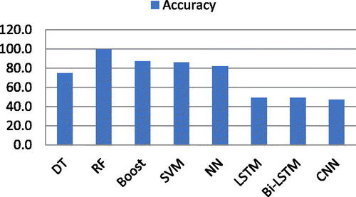
Furthermore, ML and DL classifiers were deployed for Wavelet Transform features. It was observed that RT and Boost produced 98.0% accuracy each, while SVM and DT produced 96.0% and 0.30% accuracy, respectively. On the other hand, NN, CNN, LSTM, and Bi-LSTM produced 77.0%, 54.0%,47.0%, and 49.0% accuracy respectively. Table 3 shows the accuracy results.

Table 3. Accuracy of ML and DL classifiers using wavelet transform features.

ML classifiers	Accuracy (%)	DL classifiers	Accuracy (%)
DT	96.5	NN	77.0
RF	99.6	LSTM	47.0
Boost	99.7	Bi-LSTM	49.0
SVM	98.0	CNN	54.0

Graphical representation of both ML and DL classifiers using Wavelet Transform feature list shown in Figure 6.

Figure 6. Accuracy chart of ML and DL with wavelet transform feature list.

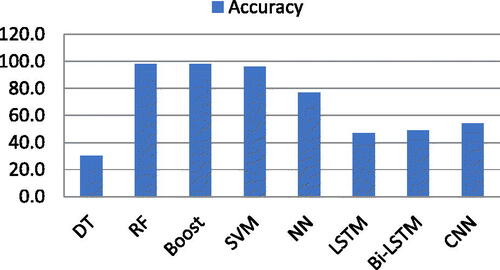
The experiments were extended using Gradient Features. ML and DL algorithms were deployed, and the results are shown in Table 4. RF performed outstandingly with 99.6% accuracy, while boost, SVM, and DT produced 87.0%, 86.0%, and 75.0% accuracy, respectively. Similarly, NN produced 82.0% accuracy while LSTM, Bi-LSTM, and CNN produced 49.0%, 49.0%, and 47.0% accuracy respectively.

Table 4. Accuracy of ML and DL classifiers using gradient features.

ML classifiers	Accuracy (%)	DL classifiers	Accuracy (%)
DT	96.5	NN	82.0
RF	99.6	LSTM	49.0
Boost	99.7	Bi-LSTM	49.0
SVM	98.0	CNN	47.0

The accuracy of ML and DL classifiers is shown in Figure 7 graphically.

Figure 7. Accuracy chart of ML and DL with gradient feature list.

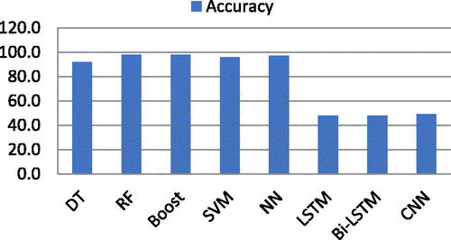
Now, ML and DL classifiers are deployed for the Autogressive feature list. It was observed that RF, Boost, SVM, and DT produced 98.0%, 98.0%, 96.0%, and 92.0% accuracy respectively. While NN showed outstanding accuracy of 97.0%. On the other hand, LSTM, Bi-LSTM, and CNN produced 48.0%, 48.0%, and 49.0% accuracy, respectively. Table 5 shows the accuracy of ML and DL classifiers using an autogressive feature list.

Table 5. Accuracy of ML and DL classifiers using autogressive features.

ML classifiers	Accuracy (%)	DL classifiers	Accuracy (%)
DT	96.5	NN	97.0
RF	99.6	LSTM	48.0
Boost	99.7	Bi-LSTM	48.0
SVM	98.0	CNN	49.0

A graphical representation of the accuracy of both ML and DL classifiers is depicted in Figure 8.

Figure 8. Accuracy chart of ML and DL with autogressive feature list.

Finally, after experiments, it was observed that ML classifiers produced good accuracy on both complete and separate feature lists of each feature. Table 6 shows the overall accuracy of both ML and DL algorithms.

Table 6. Accuracy chart of ML and DL with complete and separate feature list.

Classifiers	Accuracy (%)	Accuracy (%)	Accuracy (%)	Accuracy (%)	Accuracy (%)
	Complete features	Co-occurrence features	Co-wavelet transform features	Gradient features	Autogressive features
DT	96.5	95.0	30.0	75.0	92.0
RF	99.6	99.0	98.0	99.6	98.0
Boost	99.7	99.0	98.0	87.0	98.0
SVM	98.0	99.0	96.0	86.0	96.0
NN	50.0	93.0	77.0	82.0	97.0
LSTM	53.0	0.0	47.0	49.0	48.0
Bi-LSTM	54.0	49.0	49.0	49.0	48.0
CNN	54.0	49.0	54.0	47.0	49.0

Graphical representation of highest accuracy achieved by any classifier using complete and separate feature list shown in Figure 9.

Figure 9. Frequency table achieved by ML and DL on different feature sets.

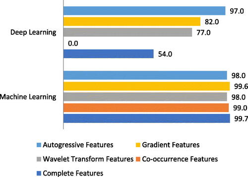
ML and DL algorithm’s classification accuracy is depicted in Figure 8. It was observed that ML classifiers obtained higher accuracy in classifying liver tumors using CT images while the accuracy produced by DL algorithms is unsatisfactory. As mentioned above, this research focuses on proving that ML algorithms produce better accuracy due to already extracted feature lists. On the other hand, DL algorithms had a separate layer named the convolutional layer responsible for feature extraction. Due to this fact, when DL algorithms took already extracted features, they produced unsatisfactory accuracy results.

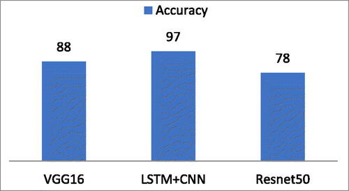
To prove this fact, pre-trained DL algorithms were deployed. This experiment deployed using LSTM + CNN, Resnet50, and VGG16. Pre-trained DL models take CT images as input and classify those images instead of taking features as input. These pre-trained DL models extract features through their available layers automatically. Experiments showed that pre-trained DL algorithms produced promising results, which were very close to ML algorithms but much better than DL algorithms. Pre-trained DL algorithms: LSTM + CNN, Resnet50, and VGG16 attained 97.0%, 78.0%, and 88.0% accuracy respectively which are shown in Table 7.

Table 7. Accuracy of pre-trained DL models.

Pre-trained DL classifiers	Accuracy (%)
VGG16	88.0
LSTM + CNN	97.0
Resnet50	78.0

The graphical representation of the pre-trained DL algorithm’s accuracy is depicted in Figure 10.

Figure 10. Accuracy chart of pre-trained DL models.

5. Discussion

As mentioned above, the focus of this research is to compare ML and DL Algorithms to check which method performed well using an already extracted features list extracted using ROI segmentation. The experiments showed that ML methods performed well using extracted features list while DL Algorithms produced poor accuracy for the identification of liver tumors using CT images. ML classifiers RF, Boost, SVM, and DT produced 99.6%, 99.7%, 98.0%, and 96.5% accuracy on a complete feature list of already extracted features. Among ML methods Boost performed outstandingly with an accuracy of 99.7%. The Boost algorithm is based on Boosting, a technique that combines numerous ‘weak’ rules—rules that may only be moderately accurate—to produce extremely accurate prediction rules. It converts week learners to strong one. This makes Boost algorithm performed outstanding among other ML algorithms (Iyer, 1999). On the other hand, DL Algorithms: NN, LSTM, Bi-LSTM, and CNN produced 50.0%, 53.0%, 54.0%, and 54.0% accuracy using the same complete feature list. DL algorithms could not be performed well on already extracted features. This happens due to its mechanism of feature extraction available in DL Algorithms in the form of layers. For validation of this, Pre-trained DL Algorithms were deployed. Instead of deploying pre-trained DL Algorithms using already extracted features, Liver CT images are directly input to the pre-trained DL Algorithms. These methods automatically extracted features using their feature extraction mechanism with the help of built-in layers. After experiments, results showed that pre-trained DL Algorithms such as LSTM + CNN, Resnet50, and VGG16 produced 97.0%, 78.0%, and 88.0% accuracy respectively as depicted in Figure 9.

This experiment strengthens the statement that ML algorithms performed well and produced better accuracy if we provide an already extracted feature list for classification while the DL Algorithms could not produce better accuracy. DL algorithms requires an enormous quantity of data to attain outstanding performance. Poor performance may result from small or inadequate data (Najafabadi et al., 2015). This may also happened due to diverse parameters. DL algorithms suffers due to limited training data or interpretability issues (Li et al., 2023). For this research, we have taken already extracted features using DL algorithms. These feature list is very limited to train DL algorithms. This may cause poor performance of DL algorithms using already extracted features. The poor accuracy of DL algorithms is specific to the problem discussed in this research by using liver tumor CT images. DL algorithms may produce poor accuracy using any other kind of image due to the fact discuss earlier that DL algorithms outperformed using huge volume of data. It means if huge volume of data may be provided to DL algorithms even in the form of already extracted features or raw images, it will performed well. On the other hand, it may produce poor results using limited amount of data in any form.

The following Table 8 show some of the recent advancements in liver tumor classification using CT images.

Table 8. State-of-the-art advancement in liver tumor classification.

Reference	Description	Accuracy
(Kumar et al. 2010)	Fuzzy C mean Clustering, Adaptive Thresholding	94.3%
(Wu et al. 2016)	Volume of Interest (VOI), Linear Iterative Clustering Approach	96.00%
(Alahmer et al. 2016)	Fuzzy C mean Clustering, SVM, Multiple ROIs	91.63%
Chang et al. (2017)	Binary Logistic Regression Analysis. Leave one out Cross Validation	81.00%
(Choi et al. 2018)	vAlexNet, VGG16,	80.00%
(Anter & Hassenian 2019)	Watershed Algorithm, Adaptive Threshold, Morphological Operationsv	95.08%
(Parsai et al. 2019)	HERMES, Likert Score, Histopathology	94.7%
(Xu et al. 2019)	Binary Logistic regression, Texture Parameters, GLCM	89.0%
(Krishan & Mittal, 2021)	Liver cancer classification, k-fold cross validation, multilevel ensemble model	87.01%
MLTI Framework (Hussain et al., 2022)	Multiclass Features Dataset & ML Algorithms	97.48%

In the future, this model may be extended to develop a hybrid model for the classification of liver tumors using CT images in which, DL Algorithms could be used for feature extraction while ML methods used for classification purposes.

6. Conclusions

ML methods produced promising results using DT, SVM, Boost, and RT using already extracted feature lists such as histogram, run-length, autoregressive, co-occurrence, gradient, and Wavelet transform. DL Algorithms such as NN, LSTM, Bi-LSTM, and CNN deployed on the complete feature lists of already extracted features. The results were unsatisfactory because DL Algorithms had their layers available for the extraction of features. That’s why, DL could not perform well on the existing feature list extracted using ROI segmentation. The liver CT images of both tumorous and no-tumorous images were taken for experiments. Pre-trained DL Algorithms were deployed to validate that DL algorithms could not perform better using already extracted features. The results produced by pre-trained DL Algorithms strengthen the above-mentioned statement.

In the future, a hybrid liver tumor classification model may be developed. In the hybrid classification method, features would be extracted using DL Algorithms and classification would be performed using ML classifiers. State-of-the-art performance on a wide range of problems has been attained by employing DL algorithms for feature extraction, one of the primary advantage of which is its capacity to handle large and complex data. However, it is computationally expensive to train and requires an enormous volume of data and computational resources. This may produce higher accuracy and the work would be expanded using other a huge dataset of imaging modalities such as MRI, X-Rays. This may increase the efficiency of proposed work by using ML algorithms for classification,

Authors’ contributions

All authors contributed equally to accomplish this study. In addition, all authors read and approved the final manuscript.

Consent to participate

Not applicable.

Consent for publication

Not applicable.

Ethical approval

Not applicable.

Acknowledgment

This research is funded by the Institute of Southern Punjab, Multan, Pakistan and University of Vaasa, Finland.

Code availability

The code will be available upon request to the corresponding author.

Conflict of interests

The authors have no conflict of interests.

Data availability

The data will be available upon request to the corresponding author.

Additional information

Funding

This work was supported by the Zhejiang Province Traditional Chinese Medicine Science and Technology Project under Grant 2024ZF106.

Notes on contributors

Mubasher H. Malik

Mubasher Malik is the Head of the Computer Science Department with the Institute of Southern Punjab. He has been involved in more than 40 publications. His main area of research are Image and Natural Languageprocessing.

Hamid Ghous

Hamid Ghous is the Head of Research for the Computer Science Department with the Institute of Southern Punjab (ISP). He is also leading the Vision, Linguistic, and Machine Learning Laboratory, ISP. He has authored and coauthored more than 30 publications in the past. His main area of research is machine and deep learningmethods.

Tahir Rashid

Tahir Rashid received the B.S. degree in computer science from Mohi ud din Islamic University Islamabad, Pakistan, in 2004, the M.S. degree in Computer Science from Muhammad Ali Jinnah University, Islamabad (M.A.J.U) in 2008. He is currently an Assistant Professor with the Department of Computer Sciences, COMSATS University Islamabad, Vehari Campus, Pakistan. His particular research interests include machine learning, data mining, software maintenance, and developing practical tools to assist softwareengineers.

Bibi Maryum

Bibi Maryum holds MBBS from University if health sciences and currently a research enthusiast. Her research interests includes AI application in gastroenterology, endocrinology and oncology.

Zhang Hao

Zhang Hao, Ph.D., is associate professor in the School of Public Health at Hangzhou Normal University. Her primary research focus on the exploration of health big data and health system simulation modeling.

Qasim Umer

Qasim Umer is working as an Assistant Professor with the Department of Computer Sciences, COMSATS University Islamabad, Vehari Campus, Pakistan. He received BS degree in Computer Science from Punjab University, Pakistan in 2006, MS degree in .Net Distributed System Development from University of Hull, UK in 2009, MS degree in Computer Science from University of Hull, UK in 2013, and Ph.D. degree from Beijing Institute of Technology, China. He is particularly interested in machine/deep learning, NLP, and IoTs. He is also interested in developing practical tools to assist software engineers.

References

- Aghamohammadi, A., Ranjbarzadeh, R., Naiemi, F., Mogharrebi, M., Dorosti, S., & Bendechache, M. (2021). TPCNN: two-path convolutional neural network for tumor and liver segmentation in CT images using a novel encoding approach. Expert Systems with Applications, 183, 115406. https://doi.org/10.1016/j.eswa.2021.115406
- Agita, T. M. (2019). Automatic liver cancer segmentation using active contour model and RF Classifier. International Journal of Innovative Technology and Exploring Engineering (IJITEE), 8, 1139–1142.
- Alahmer, H., & Ahmed, A. (2016). Hierarchical classification of liver tumor from CT images based on difference-of-features (DOF). World Congress on Engineering.
- Al Sadeque, Z. K. (2019). Automated detection and classification of liver cancer from CT images using HOG-SVM model. In 019 5th International Conference on Advances in Electrical Engineering (ICAEE) (pp. 21–26). IEEE.
- Aldeek, N. A.-Z. (2014). Liver segmentation from abdomen ct images with Bayesian model. Journal of Theoretical & Applied Information Technology, 60(3), 483–490.
- Andrade, A., Silva, J. S., Santos, J., & Belo-Soares, P. (2012). Classifier approaches for liver steatosis using ultrasound images. Procedia Technology, 5, 763–770. https://doi.org/10.1016/j.protcy.2012.09.084
- Anter, A. M., & Hassenian, A. E. (2019). CT liver tumor segmentation hybrid approach using neutrosophic sets, fast fuzzy c-means and adaptive watershed algorithm. Artificial Intelligence in Medicine, 97, 105–117. https://doi.org/10.1016/j.artmed.2018.11.007
- Bourkache, N. L. (2020) Gabor filter algorithm for medical image processing: evolution in Big Data context [Paper presentation]. In 2020 International Multi-Conference on: “Organization of Knowledge and Advanced Technologies” (OCTA), (pp. 1–4). IEEE.
- Cavalin, P. O. (2019). Confusion matrix-based building of hierarchical classification. In Progress in Pattern Recognition, Image Analysis, Computer Vision, and Applications: 23rd Iberoamerican Congress, CIARP 2018, Madrid, Spain, November 19–22, 2018, Proceedings 23 (pp. 271–278.). Springer.
- Chang, C.-C., Chen, H.-H., Chang, Y.-C., Yang, M.-Y., Lo, C.-M., Ko, W.-C., Lee, Y.-F., Liu, K.-L., & Chang, R.-F. (2017). Computer-aided diagnosis of liver tumors on computed tomography images. Computer Methods and Programs in Biomedicine, 145, 45–51. https://doi.org/10.1016/j.cmpb.2017.04.008
- Choi, K. J., Jang, J. K., Lee, S. S., Sung, Y. S., Shim, W. H., Kim, H. S., Yun, J., Choi, J.-Y., Lee, Y., Kang, B.-K., Kim, J. H., Kim, S. Y., & Yu, E. S. (2018). Development and validation of a deep learning system for staging liver fibrosis by using contrast agent–enhanced CT images in the liver. Radiology, 289(3), 688–697. https://doi.org/10.1148/radiol.2018180763
- Ciecholewski, M. a. (2007) Automatic segmentation of single and multiple neoplastic hepatic lesions in CT images [Paper presentation]. In International Work-Conference on the Interplay between Natural and Artificial Computation, 63–71.
- Dakshayani, V., Locharla, G. R., Pławiak, P., Datti, V., & Karri, C. J. (2022). Design of a Gabor filter-based image denoising hardware model. Electronics, 11(7), 1063. https://doi.org/10.3390/electronics11071063
- Das, A., Acharya, U. R., Panda, S. S., & Sabut, S. (2019). Deep learning based liver cancer detection using watershed transform and Gaussian mixture model techniques. Cognitive Systems Research, 54, 165–175. https://doi.org/10.1016/j.cogsys.2018.12.009
- Desta, A. K., Ohira, S., Arai, I., & Fujikawa, K. (2022). Rec-CNN: In-vehicle networks intrusion detection using convolutional neural networks trained on recurrence plots. Vehicular Communications, 35, 100470. https://doi.org/10.1016/j.vehcom.2022.100470
- Devi, R. M., & Seenivasagam, V. (2020). Automatic segmentation and classification of liver tumor from CT image using feature difference and SVM based classifier-soft computing technique. Soft Computing, 24(24), 18591–18598. https://doi.org/10.1007/s00500-020-05094-1
- Dwipayana, M. A. (2018). Histogram equalization smoothing for determining threshold accuracy on ancient document image binarization [Paper presentation]. In Journal of Physics: Conference Series (Vol. 1019, p. 012071). IOP Publishing. https://doi.org/10.1088/1742-6596/1019/1/012071
- Elmenabawy, N. A.-D. (2020). Deep joint segmentation of liver and cancerous nodules from CT images [Paper presentation]. In 2020 37th National Radio Science Conference (NRSC), (pp. 296–301). IEEE. https://doi.org/10.1109/NRSC49500.2020.9235097
- Ezzatollah Shrestha, U. S. (2018). Automatic Tumor segmentation using machine learning classifiers. [Paper presentation]. In 2018 IEEE International Conference on Electro/Information Technology (EIT), (pp. 0153–0158). IEEE. https://doi.org/10.1109/EIT.2018.8500205
- Fang, D., Fang, A., & Nanning, D. (2008). Image smoothing and sharpening based on nonlinear diffusion equation. Signal Processing, 88(11), 2850–2855. https://doi.org/10.1016/j.sigpro.2008.05.008
- Gao, Q., & Almekkawy, M. (2021). ASU-Net++: A nested U-Net with adaptive feature extractions for liver tumor segmentation. Computers in Biology and Medicine, 136, 104688. https://doi.org/10.1016/j.compbiomed.2021.104688
- Ghoniem, R. M. (2020). A novel bio-inspired deep learning approach for liver cancer diagnosis. Information, 11(2), 80. https://doi.org/10.3390/info11020080
- Hasan, M. E., Mostafa, F., Hossain, M. S., & Loftin, J. (2023). Machine-learning classification models to predict liver cancer with explainable AI to discover associated genes. AppliedMath, 3(2), 417–445. https://doi.org/10.3390/appliedmath3020022
- Hemalatha, V., & Sundar, C. (2021). Automatic liver cancer detection in abdominal liver images using soft optimization techniques. Journal of Ambient Intelligence and Humanized Computing, 12(5), 4765–4774. https://doi.org/10.1007/s12652-020-01885-4
- Hemalatha, G. S. (2016). Preprocessing techniques of facial image with Median and Gabor filters [Paper presentation]. In 2016 International Conference on Information Communication and Embedded Systems (ICICES), (pp. 1–6). IEEE. https://doi.org/10.1109/ICICES.2016.7518860
- Hille, G. A. (2022). Joint Liver and Hepatic Lesion Segmentation using a Hybrid CNN with Transformer Layers. arXiv preprint arXiv:2201.10981
- Hossin, M., & Sulaiman, M. N. (2015). A review on evaluation metrics for data classification evaluations. International Journal of Data Mining & Knowledge Management Process, 5(2), 01–11. https://doi.org/10.5121/ijdkp.2015.5201
- Hussain, M., Saher, N., & Qadri, S. (2022). Computer vision approach for liver tumor classification using CT dataset. Applied Artificial Intelligence, 36(1), 2055395. https://doi.org/10.1080/08839514.2022.2055395
- Iyer, R. D. (1999). An efficient boosting algorithm for combining preferences. Diss. Massachusetts Institute of Technology, 1999.” Link: “44413329-MIT.pdf
- Jabarulla, M. Y., & Lee, H.-N. (2017). Computer aided diagnostic system for ultrasound liver images: A systematic review. Optik, 140, 1114–1126. https://doi.org/10.1016/j.ijleo.2017.05.013
- Jeon, J. H., Choi, J. Y., Lee, S., & Ro, Y. M. (2013). Multiple ROI selection based focal liver lesion classification in ultrasound images. Expert Systems with Applications, 40(2), 450–457. https://doi.org/10.1016/j.eswa.2012.07.053
- Jiang, H., Zheng, R., Yi, D., & Zhao, D. (2013). A novel multiinstance learning approach for liver cancer recognition on abdominal CT images based on CPSO-SVM and IO. Computational and Mathematical Methods in Medicine, 2013, 434969–434910. https://doi.org/10.1155/2013/434969
- Jung, H. (2021). Basic physical principles and clinical applications of computed tomography. Progress in Medical Physics, 32(1), 1–17. https://doi.org/10.14316/pmp.2021.32.1.1
- Kanan, C., & Cottrell, G. W. (2012). Color-to-grayscale: does the method matter in image recognition? PLoS One, 7(1), e29740. https://doi.org/10.1371/journal.pone.0029740
- Krishan, A., & Mittal, D. (2021). Ensembled liver cancer detection and classification using CT images. Proceedings of the Institution of Mechanical Engineers. Part H, Journal of Engineering in Medicine, 235(2), 232–244. https://doi.org/10.1177/0954411920971888
- Krstinic, D. B.-S. (2020). Multi-label classifier performance evaluation with confusion matrix. Computer Science & Information Technology, 1.
- Kumar, S. S., & Moni, R. S. (2010). Diagnosis of liver tumor from CT images using curvelet transform. International Journal on Computer Science and Engineering, 2(4), 1173–1178.
- Li, W., Jia, F., & Hu, Q. (2015). Automatic segmentation of liver tumor in CT images with deep convolutional neural networks. Journal of Computer and Communications, 03(11), 146–151. https://doi.org/10.4236/jcc.2015.311023
- Li, M., Jiang, Y., Zhang, Y., & Zhu, H. (2023). Medical image analysis using deep learning algorithms. Frontiers in Public Health, 11, 1273253. https://doi.org/10.3389/fpubh.2023.1273253
- Manson, E. A. (2019). Image noise in radiography and tomography: Causes, effects and reduction techniques. Curr. Trends Clin. Med. Imaging, 2(2), 555620.
- Moghimhanjani, M. T. (2022). nalysis of liver cancer detection based on image processing. arXiv preprint arXiv:2207.08032
- Na, K., Jeong, S.-K., Lee, M. J., Cho, S. Y., Kim, S. A., Lee, M.-J., Song, S. Y., Kim, H., Kim, K. S., Lee, H. W., & Paik, Y.-K. (2013). Human liver carboxylesterase 1 outperforms alpha-fetoprotein as biomarker to discriminate hepatocellular carcinoma from other liver diseases in Korean patients. International Journal of Cancer, 133(2), 408–415. https://doi.org/10.1002/ijc.28020
- Naeem, S., Ali, A., Qadri, S., Khan Mashwani, W., Tairan, N., Shah, H., Fayaz, M., Jamal, F., Chesneau, C., & Anam, S. (2020). Machine-learning based hybrid-feature analysis for liver cancer classification using fused (MR and CT) images. Applied Sciences, 10(9), 3134. https://doi.org/10.3390/app10093134
- Naeem, H., & Bin-Salem, A. A. (2021). A CNN-LSTM network with multi-level feature extraction-based approach for automated detection of coronavirus from CT scan and X-ray images. Applied Soft Computing, 113, 107918. https://doi.org/10.1016/j.asoc.2021.107918
- Najafabadi, M. M., Villanustre, F., Khoshgoftaar, T. M., Seliya, N., Wald, R., & Muharemagic, E. (2015). Deep learning applications and challenges in big data analytics. Journal of Big Data, 2(1), 1–21. https://doi.org/10.1186/s40537-014-0007-7
- Napte, K. M. (2021). Liver segmentation and liver cancer detection based on deep convolutional neural network: A brief bibliometric survey. Library Philosophy and Practice, 1–27.
- Parsai, A., Miquel, M. E., Jan, H., Kastler, A., Szyszko, T., & Zerizer, I. (2019). Improving liver lesion characterisation using retrospective fusion of FDG PET/CT and MRI. Clinical Imaging, 55, 23–28. https://doi.org/10.1016/j.clinimag.2019.01.018
- Paulatto, L., Dioguardi Burgio, M., Sartoris, R., Beaufrère, A., Cauchy, F., Paradis, V., Vilgrain, V., & Ronot, M. (2020). Colorectal liver metastases: radiopathological correlation. Insights into Imaging, 11(1), 99. https://doi.org/10.1186/s13244-020-00904-4
- Pound, M. P., French, A. P., Murchie, E. H., & Pridmore, T. P. (2014). Automated recovery of three-dimensional models of plant shoots from multiple color images. Plant Physiology, 166(4), 1688–1698. https://doi.org/10.1104/pp.114.248971
- Rajagopal, R. S. (2015). A survey on liver tumor detection and segmentation methods. ARPN Journal of Engineering and Applied Sciences, 10(6), 2681–2685.
- Randhawa, S., Alsadoon, A., Prasad, P. W. C., Al-Dala’in, T., Dawoud, A., & ALRubaie, A. (2021). Deep learning for liver tumour classification: Enhanced loss function. Multimedia Tools and Applications, 80(3), 4729–4750. https://doi.org/10.1007/s11042-020-09900-8
- Rayan, A., Holyl Alruwaili, S., Alaerjan, A. S., Alanazi, S., Taloba, A. I., Shahin, O. R., & Salem, M. (2023). Utilizing CNN-LSTM techniques for the enhancement of medical systems. Alexandria Engineering Journal, 72, 323–338. https://doi.org/10.1016/j.aej.2023.04.009
- Razi, T. a. (2014). Relationship between Hounsfield unit in CT scan and gray scale in CBCT. Journal of Dental Research, Dental Clinics, Dental Prospects, 8(2), 107.
- Sakr, A. A. (2014). Automated focal liver lesion staging classification based on Haralick texture features and multi-SVM. International Journal of Computer Applications, 91(8), 0975–8887.
- Shah, S., Mishra, R., Szczurowska, A., & Guziński, M. (2021). Non-invasive multi-channel deep learning convolutional neural networks for localization and classification of common hepatic lesions. Polish Journal of Radiology, 86(1), e440–e448. https://doi.org/10.5114/pjr.2021.108257
- Sharma, P. (2019). Computer vision tutorial: A step-by-step introduction to image segmentation techniques. (Part 1). Retrieved from Analytics Vidhya: https://www.analyticsvidhya.com/blog/2019/04/introduction-image-segmentation-techniques-python. 2019 Apr 1
- Swaraj, K. K. (2021). Detection of liver cancer from CT images using CAPSNET. ICTACT Journal on Image and Video Processing, 12, 2601–2604.
- Tummala, B. M., & Barpanda, S. S. (2022). Liver tumor segmentation from computed tomography images using multiscale residual dilated encoder-decoder network. International Journal of Imaging Systems and Technology, 32(2), 600–613. https://doi.org/10.1002/ima.22640
- Virmani, J., Vinod, V., Kalra, N., & Khandelwa, N. (2013). PCA-SVM based CAD system for focal liver lesions using B-mode ultrasound images. Defence Science Journal, 63(5), 478–486. https://doi.org/10.14429/dsj.63.3951
- Wu, W., Zhou, Z., Wu, S., & Zhang, Y. (2016). Automatic liver segmentation on volumetric CT images using supervoxel-based graph cuts. Computational and Mathematical Methods in Medicine, 2016, 9093721–9093714. 2016. https://doi.org/10.1155/2016/9093721
- Xiong, J., Yu, D., Wang, Q., Shu, L., Cen, J., Liang, Q., Chen, H., & Sun, B. (2021). Application of histogram equalization for image enhancement in corrosion areas. Shock and Vibration, 2021, 1–13. https://doi.org/10.1155/2021/8883571
- Xu, X.-F., Xing, H., Han, J., Li, Z.-L., Lau, W.-Y., Zhou, Y.-H., Gu, W.-M., Wang, H., Chen, T.-H., Zeng, Y.-Y., Li, C., Wu, M.-C., Shen, F., & Yang, T. (2019). Risk factors, patterns, and outcomes of late recurrence after liver resection for hepatocellular carcinoma: A multicenter study from China. JAMA Surgery, 154(3), 209–217. https://doi.org/10.1001/jamasurg.2018.4334
- Yankovy, I. I. (2021). Classifier of liver diseases according to textural statistics of ultrasound investigation and convolutional neural network. CEUR Workshop Proceedings, 60–69.
- Zhang, Y. W. (2020). Deep learning and unsupervised fuzzy C-means based level-set segmentation for liver tumor [Paper presentation]. In 2020 IEEE 17th International Symposium on Biomedical Imaging (ISBI), (pp. 1193–1196). IEEE. https://doi.org/10.1109/ISBI45749.2020.9098701
- Zhou, J. W., Lei, B., Ge, W., Huang, Y., Zhang, L., Yan, Y., Zhou, D., Ding, Y., & Wu, J. (2021). Automatic detection and classification of focal liver lesions based on deep convolutional neural networks: a preliminary study. Cancer Imaging and Image-directed Interventions – Frontiers, 10, 581210.