Performance evaluation and CFD investigation of scraped surface ice cream freezer augmented with LN₂ freezing technique

Abstract

Ice cream is a frozen mixture comprising milk, cream, sugar, milk solids-not-fat, stabilizers, and emulsifiers. This study explores the production of ice cream using a Scraped Surface Freezer (SSF) combined with a liquid nitrogen (LN₂) freezing technique. The innovative approach involves utilizing liquid nitrogen as a refrigerant and employing gaseous nitrogen released during heat transfer to control the overrun in the final ice cream product. The experimental investigation of SSF involved examining the draw temperature of ice cream and determining its overall heat transfer coefficient. The drawing temperature of −6 °C and overall heat transfer coefficient close to 300 W/(m²°C) was obtained after the process optimization. To better understand what occurs inside SSF, numerical simulation using ANSYS Fluent was used to acquire the flow parameters such as temperature, pressure, and velocity. The flow profile was obtained under the reference operating conditions: feed flow rate = 240 lit/hr, LN₂ temperature = −95 °C, and scraper speed =125 rpm. The computational Fluid Dynamics (CFD) results reveal confined flow between blades and the inner heat transfer tube surface, causing a directional velocity change. Due to this recirculation, a faster decrease in temperature was observed in this area. The results of the experimental investigation of the SSF were rigorously compared with the CFD results. Based on numerical simulations, the initial freezing point in SSF occurred at an axial distance of 0.2 m.

Keywords:

• Ice cream
• scraped surface freezer
• liquid nitrogen
• heat transfer
• computational fluid dynamics

Reviewing Editor:

• Pham D T, University of Birmingham, United Kingdom

Subjects:

• Food Analysis
• Food Engineering
• Agriculture and Food

1. Introduction

Due to the simplicity of cooking with frozen foods and their long-term preservation, their consumption has significantly increased. Due to the market’s increasing need for high-quality frozen meals, refrigeration engineering and technology must be improved (Kim et al., 2014). As a result, there is a need for the creation of continuous freezers with large capacity and low cost. The market already offers a variety of batch and continuous freezers (Shrivastav and Goswami, 2018). To treat semi-solid foods like ice cream, sorbets, etc. as well as highly viscous non-Newtonian fluids, scraped surface freezers (SSF) are typically utilized. Rotor and blade assembly, a heat transfer tube, and a freezer barrel (Jacket) are all included in SSFs. Due to an axial pressure gradient along the annulus, the product to be frozen flows inside the heat transfer tube. To prevent fouling and maintain the proper heat transfer rate, blades attached to the shaft scrape off the frozen material from the inner wall. To remove heat from the product that needs to be frozen, the refrigerant passes through the outer jacket. To rotate at the desired speed, the shaft is fastened to the motor and gearbox.

Huggins (1931) developed the concept of a scraped surface heat exchanger (SSHE) and observed that using scrapers when processing viscous fluids significantly improves the heat transfer coefficient. Numerous studies investigated the impact of improved heat transmission in the heat exchanger’s scraping surface side using theoretical and/or empirical methods. From penetration theory, Kool (1958), Latinen & Skelland (1959), and Harriott (1959) derived a theoretical model for calculating the heat transfer coefficient on the scraper side. Skelland (1958) developed an empirical method for calculating the internal heat transfer coefficient using dimensional analysis. The developed model was then refined by Skelland et al. (1962), and it now closely matches the results from the penetration hypothesis. Some of the other researchers who worked on scraped surface heat exchangers by taking into account various aspects involved in heat and exchanger and then based on that had developed various models include Penney and Bell (1967), Trommelen et al. (1971), De Goede and De Jong (1993), Boccardi et al. (2008), Boccardi et al. (2010), Saraceno et al. (2011), and Varga et al. (2017). However, only a small number of scholars, according to Lee and Singh (1990), have investigated how to determine the heat transfer coefficient when fluid dynamic phase change (crystallization) is involved. Following this, other investigations involving the freezing of an aqueous solution including phase change and scraped surface heat exchangers have been published (Lakhdar et al., 2005; Qin et al., 2003, 2006).

Computational Fluid Dynamics (CFD) is a numerical approach used to determine the behavior of fluid flowing inside the SSHE. CFD simulation has a broad range of applications within the food processing industry (Szpicer et al., 2023). Numerous studies have also been conducted to perform CFD analysis of SSHE. Yataghene et al. (2008) conducted a numerical investigation to examine the flow patterns and shear rate across the SSHE. Yataghene and Legrand (2013) conducted a numerical study to compare the thermal properties distribution of non-Newtonian fluid and Newtonian fluid at different mass flow rates and blade speed combinations. The 3D-numerical simulation was solved for momentum, energy, and continuity equations with the code developed on FLUENT 6.3. Ali and Baccar (2017) studied the numerical simulation in the case of SSHE which is equipped with helical ribbons instead of scraper blades. The effect of the ratio of rotational to axial Reynolds number and Oldroyd number on the thermal and hydrodynamic behaviors was studied. Hernández-Parra et al. (2018) studied non-aerated sorbet flow in a pilot-scale scraped surface heat exchanger (SSHE) under various conditions. They used Computational Fluid Dynamics (CFD) to solve momentum, energy, and continuity equations. Analyzing velocity, temperature, and pressure, they investigated flow behavior at different mass flow rates and rotor speeds within the SSHE. Mukesh Kumar and Chandrasekar (2019) studied the numerical simulation of a double helical tube type heat exchanger as it was found that the helical tube type results in the enhancement of the heat transfer as compared to the straight tubes due to the increase of turbulence.

The device that was created utilized liquid nitrogen (LN₂) as a freezing medium. The usual boiling point of LN₂ is −195.8 °C (77 K; −320 °F), and it has a density of 808 kg/m³. LN₂ works in the temperature range of −60 °C to −120 °C (Kumar et al., 2018). The creation of very small ice crystals at the substantially lower temperature of LN₂ leads to uniform distribution of the product and a faster rate of freezing or rapid heat transfer, both of which enhance the quality of the frozen product (Zhu et al., 2019). As a result, heat can be carried by conduction to the ice layer that has developed on the surface of the wall due to the substantial temperature difference between the ice cream mix and LN₂.

Based on existing scientific investigations, several notable research gaps have been recognized in the domain of ice cream production. First, the utilization of liquid nitrogen as a refrigerant within the Scraped Surface Freezer for ice cream manufacturing remains unexplored. Second, the simultaneous introduction of nitrogen gas into the ice cream mixture within the Scraped Surface Freezer to achieve the desired overrun has not been previously attempted. Finally, there is a notable absence of studies examining the production of ice cream using liquid nitrogen within a continuous freezer setup.

The SSF freezer used here for ice cream production utilizes LN₂ as a refrigerant, which flows inside the jacket. After heat transfer, the emerging nitrogen gas is injected into the ice cream mixture to achieve the desired overrun. A performance study of the SSF was conducted under various operating conditions, followed by process optimization to determine the reference operating condition. Subsequently, CFD analysis was performed to assess the flow properties of ice cream inside the heat transfer tube. Finally, the experimental results were compared with the CFD results.

2. Material and methods

2.1. The Scraped Surface Freezer

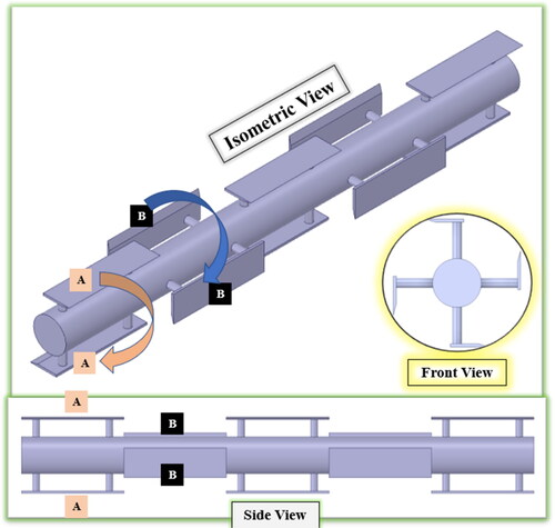
Figure 1 shows the process and flow diagram of the ice cream making process in SSF. The diagram shows all the connections made for carrying out the experiment. The SSF is about 0.7 m in length as shown in the diagram with the provisions of all the inlets, outlets, and connections. The shaft inside the freezer is connected with the blades that are arranged 180° to each other as shown in Figure 2. The isometric view, front view, and side view of the blade and rotor assembly can be seen in this figure. From the figure, it can be seen that the blades are arranged in such a manner that blades A–A and B–B are 180° to each other, while A–B blades are 90° to each other. The side view shows that there is no gap between the end of the A–A blades and the start of the B–B blades. This will ensure that the scraping of the entire surface of the heat transfer tube takes place. Such types of arrangements also enhance the mixing effect. The blade and shaft assembly were operated with the help of a 3-phase induction motor (M). Gear Box (G) is connected to the motor for the speed reduction. The control panel (E) records the motor speed and can be observed in the display of the control panel. The switchboard is also provided for operating the centrifugal pump and running the compressor. Another switchboard is also provided for carrying out the various operations in the scraped surface freezer via a control panel.

Figure 1. Process and flow diagram for the connections made in SSF.

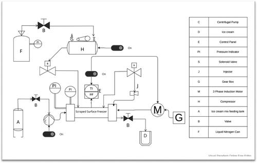
Figure 2. Isometric view, front view, and side view of the blade and rotor assembly.

Ice cream mix feeding tank (A), manually operated valve (B), and centrifugal pump (C) represent the mechanism for feeding ice cream mix into the inlet of the freezer. The outlet side of the freezer is also connected to a manually operated valve (B) and a tank for collecting ice cream (D). A separate pressure indicator (PI) is provided for measuring pressure both inside the heat transfer tube and jacket side of the freezer.

A separate mechanism is provided to supply liquid nitrogen at the inlet of the jacket side of the freezer. F represents the cryo-can filled with LN₂, which is also attached to the pressure indicator. Compressor (H) compresses the LN₂ towards the solenoid valve (S), which then goes inside the jacket side of the freezer. The jacket was properly insulated with a sheet of polyethylene foam to resist heat transfer to the environment. Polyethylene foam is an excellent insulator and found to be very suitable for SSF as it can be bent in any shape. A solenoid valve (S) is also provided at the other end of the jacket, which collects the gaseous nitrogen-containing vapors (due to heat transfer). The nitrogen is then ejected inside the heat transfer tube with the help of an injector (J) to volumize the ice cream or to provide a certain amount of overrun in the ice cream.

2.2. Ice cream mix formulation and preparation

Ice cream mixes were formulated to contain 12% (w/w) fat, 11% (w/w) MSNF, 14.5% (w/w) sugar, 0.4% (w/w) stabilizer, and 0.3% (w/w) emulsifier. To achieve the desired composition as mentioned, a simple algebraic method was used for each formulation. For this Amul Taza Homogenized toned milk having 3% fat and 8.5% MSNF, and Amul Fresh cream having 25% fat and 3.4% MSNF were used. Skim Milk Powder (SMP) with 1.5% fat and 96% MSNF was used to get the desired total solid concentration in ice cream. Gelatin was used as a stabilizer; Tween 80 was used as an emulsifier. This makes the total solid content of the final mixture 38.2%. The whole milk was initially blended with granulated sugar (purchased from the local market) and skim milk powder (SMP, Loba Chemie Pvt. Ltd. Mumbai, MH). The cream was then whipped with the commercial blender to give the ice cream a smooth texture and creamy taste and was added to the initially blended mixture of whole milk, sugar, and SMP. After this, Tween 80 (Polyoxyethylene sorbitan monooleate) (Merk Specialities Pvt. Ltd. Mumbai, MH) whose density varies from 1.06 to 1.09 gm/ml, and Gelatin powder (Loba Chemie Pvt. Ltd. Mumbai, MH) was added to the mixture. The mixture was then gently stirred for a uniform mix and kept in an ice bath to cool down. After this, the ice cream mix was placed in a deep freezer for aging at 4 °C overnight (24 hrs.).

2.3. Experimental procedure

The formulated ice cream mixture is first poured into the ice cream mix feeding tank. Before starting the experiment, it was made sure that all the connections were properly done for the smooth operation of the system. Initially, compressor was started and LN₂ was allowed to enter the jacket side of the freezer. The jacket was also provided with the manually operated valve, which was checked throughout the experiment so that the pressure inside the jacket didn’t build up. At the same time, the motor was started to rotate the shaft and blade assembly at a certain rpm. Once the jacket was filled, the ice cream mix at 4 °C was allowed to enter the freezer by running the centrifugal pump. After this, the solenoid valve at the exit side of the jacket was opened so that the evaporating nitrogen goes inside the heat transfer tube which is filled with an ice cream mixture. As nitrogen is inert and non-toxic, it can be safely used for creating the desired amount of overrun in ice cream. The frozen and aerated ice cream that was coming out of the freezer was then collected at the outlet of the freezer and used for further analysis.

The process parameters like feed flow rate, scraper speed, and LN₂ temperature were analyzed using an ice cream mixture as feed. This analysis of variance (ANOVA) was conducted using design expert software. Drawing temperature and overall heat transfer coefficient were considered as the measure of optimization. The experiment was conducted under different operating conditions as shown in Table 1. The optimum value of the desirable drawing temperature and optimum overall heat transfer coefficient at the process parameter condition was obtained.

Table 1. Independent variables selected for optimization process for ice cream mixture as feed.

Process parameters (factors)	Values
A: Feed flow rate	200 to 240 lit/hr
B: Scraper speed	125 rpm (kept constant)
C: Liquid nitrogen temperature	−95 to −75 ˚C

2.4. Physical problem description for CFD analysis

Initially, it is important to describe the physical problem before carrying out further analysis. The SSF consists of two concentric cylinders with the inner cylinder acting as a heat transfer tube having a diameter of 0.12 m and a length of 0.7 m. The rest of the geometrical characteristics are given in Table 2. The geometry of the SSF adapted to carry out the CFD analysis is shown in Figure 3. The ice cream mix enters the freezer at a temperature of 4 °C, which was kept fixed throughout the experiment.

Figure 3. Geometry of SSF.

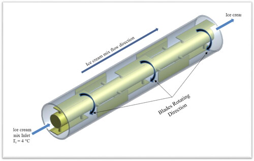
Table 2. Geometrical characteristics of SSF.

Geometrical parameters	Symbol	Value
Length of the heat transfer tube	L	0.7 m
Inside diameter of the heat transfer tube	Dt	0.12 m
Outside diameter of the heat transfer tube	Do	0.128 m
Thickness of the heat transfer tube	t	0.004 m
Rotor or shaft diameter	Ds	0.05 m
Inside jacket diameter	Dj	0.168 m
Outside jacket diameter	Dj2	0.180 m

To simplify the simulation and facilitate the analysis of flow properties within the freezer, we only considered the LN₂ temperature as the free stream temperature applied to the outer surface of the heat transfer tube for numerical simulation. We did not simulate the flow of LN₂ inside the jacket. The simulation inside the heat transfer tube was carried out for the optimized range of process parameters conditions obtained earlier.

2.5. Governing equations

Although ice cream is a multiphase product in which ice, fat, and air are present as discrete phases surrounded by concentrated aqueous solution (serum), in the present study, it was assumed as a single-phase fluid, with apparent physical properties varying with temperature. Therefore, the approach proposed by Lakhdar et al. (2005) used in this study, uses the conservation equations of mass, momentum, and energy for single-phase fluid. In SSF, the heat transfer tube and blade with shaft are the most important parts of the freezer. Due to the presence of rotating elements, it will be more convenient to establish the governing equation using a rotating reference frame since it takes into account non-moving elements. The velocity in the moving frame ($\overrightarrow{\mathrm{v}}$) can be represented with the help of velocity in the Galilian frame ($\overrightarrow{\mathrm{u}}$) as given in Equation (1)(1) $$\overrightarrow{\mathrm{u}}=\overrightarrow{\mathrm{v}}+\overrightarrow{\mathrm{\Omega }}\times \overrightarrow{\mathrm{r}}$$(1) . (1) $$\overrightarrow{\mathrm{u}}=\overrightarrow{\mathrm{v}}+\overrightarrow{\mathrm{\Omega }}\times \overrightarrow{\mathrm{r}}$$(1)

Any type of fluid flow can be described with the governing equations of continuity, Navier–Stokes (N–S), or momentum and energy which is based on the conservation of mass, momentum, and energy. The fluid flow problems can be solved with the set of governing equations by having proper initial and boundary conditions. The governing equation for mass, momentum, and energy can be given as (2) $$\overrightarrow{\nabla }\bullet \overrightarrow{\mathrm{v}}=0$$(2) (3) $$\mathrm{\rho }\left(\overrightarrow{\mathrm{v}}\bullet \overrightarrow{\nabla }\right)\overrightarrow{\mathrm{v}}=-\overrightarrow{\nabla }\bullet \stackrel{̿}{\mathrm{\tau }}-\overrightarrow{\nabla }\mathrm{p}-2\mathrm{\rho }\left(\overrightarrow{\mathrm{\Omega }}\times \overrightarrow{\mathrm{v}}\right)-2\mathrm{\rho }\left(\overrightarrow{\mathrm{\Omega }}\times \overrightarrow{\mathrm{\Omega }}\times \overrightarrow{\mathrm{r}}\right)$$(3) (4) $$\rho C_p\overrightarrow{v}\bullet \overrightarrow{\nabla }\mathrm{ }\mathrm{T}=\overrightarrow{\nabla }\bullet \left(\mathrm{k}\mathrm{ }\overrightarrow{\nabla }\mathrm{ }\mathrm{T}\right)-\left(\stackrel{̿}{\mathrm{\tau }}:\overrightarrow{\nabla }\mathrm{ }\overrightarrow{\mathrm{v}}\right)$$(4) where, $\overrightarrow{\mathrm{v}}$ = Velocity (m/s); $\stackrel{̿}{\tau }$ = viscous stress tensor obtained from power-law model; p = pressure (Pa); T = temperature (°C); ρ = density (kg/m³); C_p = specific heat capacity (J/(kg°C)); k = thermal conductivity (W/(m°C)); Ω = rotating speed of the rotor and blade assembly.

In this research article, the effect of scraper blades and rotor was considered while carrying out the CFD analysis while the effect of supports of blades on the rotating shaft and the support of the rotor were ignored, considering it the negligible portion of the freezer. In relation to the rotating reference frame, the rotor and blades appear to be static, therefore, the equation of heat transfer becomes (5) $$\overrightarrow{\nabla }\bullet \left(\mathrm{k}\mathrm{ }\overrightarrow{\nabla }\mathrm{ }\mathrm{T}\right)=0$$(5)

2.6. Solution methodology

The governing equations were solved using ANSYS Fluent 18.0 (Canonsburg, Pennsylvania, U.S) and the assumptions made to carry out the numerical investigation are as follows:

1. A steady-state condition was assumed while operating the freezer.

2. The heat transfer surface was assumed to be free from fouling throughout the numerical investigation.

3. The fluid was assumed to remain in a single phase while carrying out the CFD analysis.

4. In a specific simulation run, the temperature of the LN₂ applied to the surface of the heat transfer tube was assumed to be constant.

5. The frictional losses due to the movement of the scraping blades or other mechanical components within the heat exchanger were ignored in the simulation study.

The primary objective of the modified methodology was to achieve a desired outlet temperature of −6 °C in the freezer. Consequently, the scraped surface freezer (SSF) was simulated under various operating conditions, including rotor speed, feed flow rate, and LN₂ temperature, to attain the target outlet temperature.

2.7. Boundary conditions

The CFD code was developed in Ansys Fluent 18.0 (Canonsburg, Pennsylvania, U.S), and the following boundary conditions were assumed before performing the CFD analysis:

1. The ice cream mix enters the freezer at the constant inlet temperature of 4 °C.

2. The heat transfer wall temperature was assumed to remain at a constant uniform temperature when carrying out that particular simulation.

3. At the outlet of the freezer, the null gradient of temperature was assumed for the ice cream mix.

4. No slip condition was assumed at the inner wall of the heat transfer tube and inlet and outlet condition, and with respect to the rotating reference frame they are moving at a speed equal to the speed of rotation of the shaft and rotor assembly, therefore, the equation of no-slip condition will become (6) $$\overrightarrow{v}=-\overrightarrow{\mathrm{\Omega }}\times \overrightarrow{\mathrm{r}}$$(6)

5. No slip condition was assumed at the blade and rotor surface. Hence, $\overrightarrow{v}=0.$

6. The outflow boundary condition was assumed at the outlet.

2.8. Product physical properties

Ice cream’s physical properties must be known before carrying out the CFD analysis. It can be found out experimentally or by using empirical models by keeping some assumptions to get close approximated results. The specific heat was calculated by using Chen’s (1985) model while the thermal conductivity and density were calculated using Choi and Okos’s (1986) model for varying temperature conditions. The values of density, specific heat, and thermal conductivity obtained at different static temperatures were fitted in the piecewise linear model and were obtained in the form of a linear curve as shown in Figure 4. For obtaining the viscosity values, a non-Newtonian power law model was applied, which was varying as a function of strain rate and static temperature. The power law model was used to describe the rheological properties of the ice cream mix. The flow behavior index (n) and the consistency index (K) values were obtained by fitting the rotational speed versus the apparent viscosity values to the power law model. $${\mathrm{\eta }}_{\mathrm{a}}={\text{K}\mathrm{\gamma }}^{(\mathrm{n}-1)}$$

Figure 4. Model fitted curve for the variation of (a) specific heat, (b) density, (c) thermal conductivity, and (c) viscosity with static temperature obtained in ANSYS Fluent.

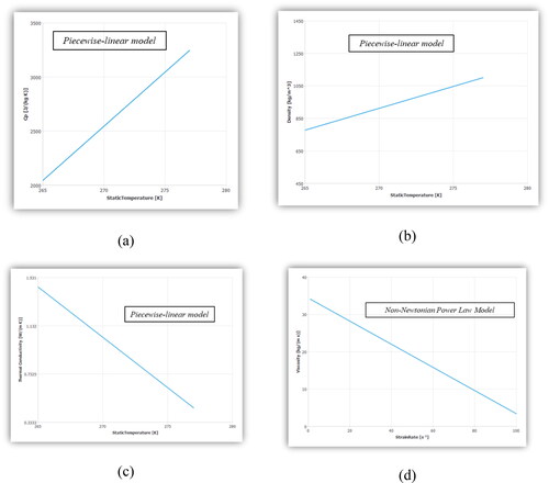
where η_a is the apparent viscosity (Pa.s); K (Pa.sⁿ) is the consistency index; γ is the rotational speed (s⁻¹); and n (dimensionless) is the flow behavior index. However, the viscosity of ice cream and ice cream mixes greatly depends on the mix composition, processing and handling of the mix, total solid content, temperature, etc. (Bahramparvar & Mazaheri Tehrani, 2011). Additionally, the percentage concentration of stabilizer plays an important role in affecting the viscosity of ice cream (Shrivastav et al., 2022). Typically, K values for ice cream range from around 0.1 to 100 Pa·sⁿ, depending on factors such as the fat content, stabilizers, emulsifiers, and other ingredients used. For ice cream mixes, n values usually fall within the range of 0.1 to 0.7, indicating that the viscosity decreases with increasing shear rate. To conduct the simulation, we used a value of 5 Pa·sⁿ for K and a value of 0.5 for n. In the present study, we did not consider how physical properties change during freezing, but in the future, we can explore this to understand how flow properties like viscosity change. This knowledge is crucial for understanding how different factors impact fluid flow, which has broad applications.

The constant value of the thermal properties of LN₂ (Table 3) was obtained from the fluent database and used for carrying out the numerical simulation.

Table 3. Thermal properties of LN₂ obtained from fluent database.

Density [kg/m^3]	Specific heat [J/(kg K)]	Thermal conductivity [W/(mK)]	Viscosity [kg/(ms)]
806.08	2041.5	0.14581	0.00016065

The constant value of the thermal properties of steel (Table 4) was obtained from the fluent database and used for carrying out the numerical simulation.

Table 4. Thermal properties of solid material (steel) applied from the fluent database.

Density [kg/m^3]	Specific heat [J/(kg K)]	Thermal conductivity [W/(mK)]
8030	502.48	16.27

2.9. Meshing

The meshing of the developed geometry was done in the ANSYS Meshing Tool. The tetrahedral meshing of each part of the SSF was done as shown in Figure 5.

Figure 5. Tetrahedral meshing of (a) blade and rotor assembly (b) around the surface of heat transfer tube and the jacket.

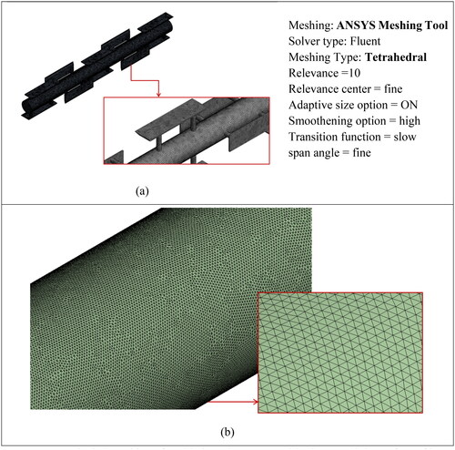
The computational fluid dynamics (CFD) simulation was conducted using the ANSYS Meshing Tool with Fluent as the solver. The geometry modeling involved creating a digital representation of the system under study. The grid generation process included the use of adaptive sizing with the ‘ON’ option to generate an assembly mesh. A relevance setting of 10 was applied, with a fine relevance center to ensure grid refinement. Additionally, the smoothening option was set to high, and a slow transition function was employed to optimize mesh quality. To ensure proper grid arrangement, the fine span angle center operation was selected. These steps were taken to accurately model the geometry, generate a high-quality grid, and set up the CFD simulation for reliable results.

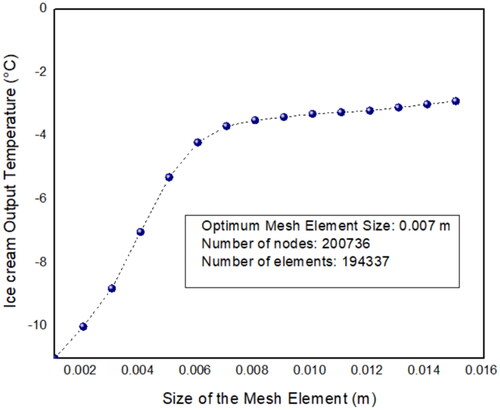
In numerical simulations, efficiency and accuracy are crucial parameters. At times, prioritizing higher accuracy may lead to compromising computational efficiency. To ensure higher accuracy, it becomes essential to conduct a grid independence test. This test involves a series of simulations aimed at determining the mesh or grid size where its impact on the results is minimal. Various simulations were conducted, adjusting the element size to achieve grid-independent results.

A parametric analysis was conducted, considering mesh element size, number of nodes, and number of elements as input parameters, while the output temperatures of ice cream and liquid nitrogen served as the output results. The mesh element size varied from coarse to finer, ranging from 0.015 m to 0.001 m. The impact of mesh element size on the ice cream’s drawing temperature was investigated, as depicted in Figure 6. The optimal element size was determined to be 0.007 m, as minimal changes in output temperature were observed upon further mesh refinement beyond this size. Correspondingly, the number of nodes and elements for this mesh size were found to be 200,736 and 194,337, respectively.

Figure 6. The relationship between ice cream output temperature and mesh element size variation.

2.10. Solving and post processing

Fluent was used as a computational method to solve the numerical simulation of the process inside the SSF. The code in the ANSYS Fluent uses the Finite Volume Method (FVM) for discretization. The surface and volume integrals of the steady-state Navier-Stokes equations are applied to each surface and control volume of the domain. A computational node is present at the centroid of each tetrahedral mesh element which solves the partial differential equation (PDE) of the Navier-Stokes equations. The double precision option with the serial-based processing system was enabled while activating the ANSYS Fluent Launcher to get quick and accurate results. In the solver, check the mesh to make sure that the minimum volume is not negative. The pressure-based steady-state solver was used and the energy equation was turned on. The fluid material was assigned in the fluid domain in the cell zone condition and the boundary conditions were set. The pressure–velocity coupling was done using the SIMPLEC Algorithm. A second-order upwind interpolation scheme was used for the energy equation. The hybrid initialization was done in order to quickly initialize the solution. The convergence criteria were set to 1e − 06 residuals for all cases. For each trial, at least 500 iterations were performed and the convergence was reached at around 300 iterations in each case. The flow properties like temperature, pressure, and velocity change w.r.t flow rate and liquid nitrogen temperature were calculated.

3. Results and discussion

3.1. Experimental process optimization

When circulating the ice cream mixture inside the freezer, the effect of process parameters on dependent variables like drawing temperature and overall heat transfer coefficient was studied. The drawing temperature (T) and overall heat transfer coefficient (U) were found to vary with feed flow rate (A), and temperature of LN₂ on the jacket side (C) at a constant rotor speed of 125 rpm. The second-order polynomial regression equations for the relationship between dependent and independent variables (in terms of coded factors) are given as (7) $$\text{Drawing Temperature} \left(\mathrm{T}\right)=-4.50+0.77*\text{A}+0.69*\text{B}+0.000*\mathrm{A}*\text{B}+0.22*{\mathrm{A}}^2-0.097*{\mathrm{B}}^2$$(7) (8) $$\text{Overall Heat Transfer Coefficient}\left(\mathrm{U}\right)=+324.86+22.45*\text{A}+32.80*\text{B}+2.02*\mathrm{A}*\text{B}-2.5*{\mathrm{A}}^2+4.65*{\mathrm{B}}^2$$(8) 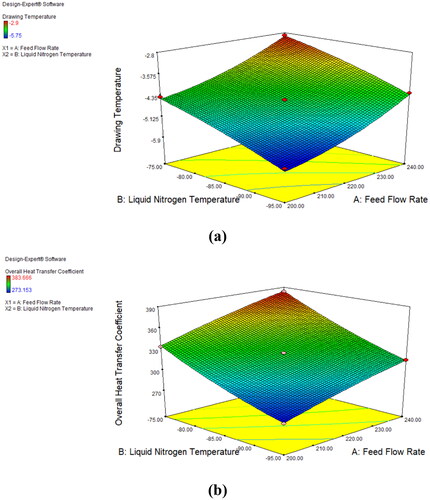where, T is the drawing temperature in °C, U is the Overall Heat Transfer Coefficient in W/(m²°C). The optimization criteria were set to drawing temperatures lower than −6 °C in the experiment conducted and the maximum possible heat transfer coefficient. Figure 7 represents the three-dimensional contour plot of the variation of drawing temperature and overall heat transfer coefficient with feed flow rate and liquid nitrogen at a constant rotor speed of 125 rpm. The quadratic model was applied and results were considered significant for p < .0001. The Predicted R-squared value of 0.9753 was in reasonable agreement with the Adjusted R-squared value of 0.9940. In Figure 7(a), it can be seen that the drawing temperature lowers at lower Liquid Nitrogen temperature, while an increase in feed flow rate increases the drawing temperature due to less residence time in the freezer, thereby reducing the time of contact between the mixture and heat transfer wall. It can also be observed from Figure 7(b) that the value of the overall heat transfer coefficient dropped with a decrease in LN₂ temperature due to the drop in drawing temperature and thereby, an increase in temperature difference between the inlet and outlet of the freezer due to lowering of LN₂ temperature. Increasing the feed flow rate results in an increase in the overall heat transfer coefficient and a gentle increase in the overall heat transfer coefficient with an increase in feed flow rate was observed.

Figure 7. Effect of feed flow rate and LN₂ temperature on the (a) drawing temperature and (b) overall heat transfer coefficient at scraper speed of 125 rpm.

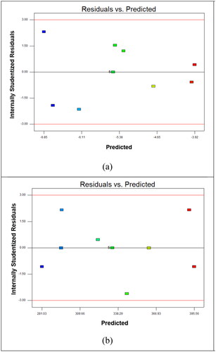
To assess the accuracy of the conducted experiments, a plot between internally studentized residuals and predicted values was examined to detect any constant errors. Figure 8(a) and (b) shows the scatter plot between internally studentized residuals and predicted values for the drawing temperature and overall heat transfer coefficient as the response variables, respectively. Residuals are the differences between the observed values of the response variable and the values predicted by the regression model. Internally studentized residuals are a standardized form of residuals. They are calculated by dividing each residual by an estimate of its standard deviation, which is computed without including the data point being analyzed. The predicted values represent the response variable’s estimated values generated by the regression model for every combination of predictor variables. To detect any errors, threshold residual values were set at +3 and −3 for both cases. It was evident from the scatter plot that the residual values fell within the threshold range, indicating that they do not significantly affect the regression model analysis.

Figure 8. Scatter plot illustrating the relationship between internally studentized residuals and Predicted values for the (a) drawing temperature and (b) overall heat transfer coefficient as the response variables.

The drawing temperature of −6 °C and an overall heat transfer coefficient close to 300 W/(m²°C) were obtained at the boiling LN₂ temperature of −95 °C and a feed flow rate of 220 lit/hr. According to the study done by Qin et al., an overall heat transfer coefficient close to 200 W/m²°C was obtained when conducting heat transfer during the freezing of an aqueous solution involving phase change. Therefore, a good overall heat transfer coefficient was achieved for the drawing temperature of −6 °C.

3.2. CFD results obtained by parametric analysis

The SSF augmented with liquid nitrogen was simulated and flow properties like temperature, pressure, and velocity change with respect to flow rate, LN₂ temperature inside the jacket, and rotor speed were obtained at the inlet, outlet, and throughout the freezer. For this, the parametric analysis was done in order to obtain the desirable output values. By keeping the LN₂ temperature flowing inside the jacket constant, i.e. −95 °C (at which we are getting the desirable drawing temperature of −6 °C after experimental process optimization), flow properties values were again examined for varying feed flow rate and scraper speed. Figure 9 shows the CFD results obtained at feed flow rates of 200 lit/hr, 220 lit/hr, and 240 lit/hr, scraper speed varying from 100 rpm to 125 rpm (at an interval of 5 rpm), and constant LN₂ temperature of −95 °C.

Figure 9. CFD parametric results obtained for the (a) output temperature condition, (b) velocity, and (c) pressure drop with varying feed flow rate and scraper speed.

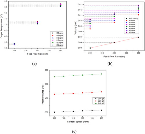
From Figure 9(a), it can be seen that output temperature, i.e. −6 °C was obtained at the feed flow rate of 240 lit/hr and scraper speed of 125 rpm. It was observed that for the same feed flow rate, there was a slight lowering in drawing temperature was found by increasing the scraper speed. This lowering of output temperature may be due to the increase in the rate of heat transfer due to subsequent scraping action.

Figure 9(b) shows the graphical form of changes in inlet and outlet velocity conditions for varying feed flow rate and scraper speed. It can be seen that the velocity at the inlet remained constant for that particular feed flow rate but at the outlet, the velocity increases with an increase in feed flow rate. Also, with an increase in scraper speed, the outlet velocity further increases due to v = r.ω, where ω is the angular speed of the rotor. As explained earlier, the increase in velocity due to an increase in feed flow rate was due to an increase in pressure drop. Also, the pressure drop values with feed flow rate and scraper speed were also observed as shown in Figure 9(c). As the ice cream mixture precedes toward the outlet, the scraper motion results in a lowering of pressure inside the heat transfer tube which results in a slight decrease at the outlet, thereby increasing the pressure drop. As the scraper motion increases, the pressure at the outlet further lowers enhancing the pressure drop value.

3.3. Analysis of flow profiles

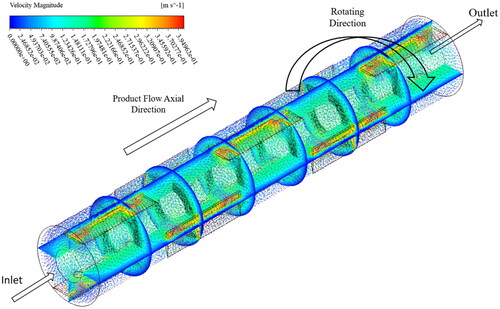
The fluid flow phenomenon of the SSF is shown in Figure 10, where the velocity magnitude was described at the different planes of the freezer. This flow profile was obtained under the reference operating conditions: feed flow rate = 240 lit/hr, LN₂ temperature = −95 °C, and scraper speed =125 rpm. The rotation direction of the scraper blades was clockwise as shown in the figure. The highest velocity can be observed in the vicinity of the outer surface area of the blades. The flow is confined between blades and the inner heat transfer tube surface, and as a consequence change in the velocity direction was found at that area. Duffy et al. (2007) also predicted in their study, the recirculation of fluid flow near the endings of the blade by conducting the mathematical modeling of fluid flow in heat exchangers of scraped surface type. Due to this recirculation, a faster decrease in temperature can be observed in the case of the product confined in the area between the heat transfer tube wall and the blade surface.

Figure 10. Velocity field in SSF obtained under reference operating conditions as predicted by numerical modeling.

3.3.1. Velocity profile distribution

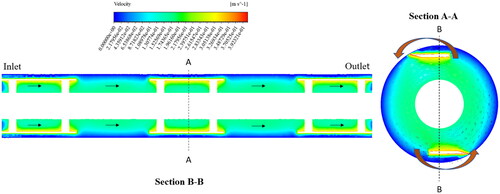
Figure 11 displays that the product flows from inlet to outlet (left to right) as indicated by the arrows (sectional plane B–B, left side). The low velocity can be observed in the vicinity of the heat transfer wall due to retarding shear force acting in the direction opposite to the fluid flow, while the higher velocity can be seen on the surface of the blades. At the surface of the blade, the product flow experiences the effect of both linear and angular velocity. In the sectional plane A–A (right side figure), it can be seen with the help of the velocity vector that as the blades rotate the high-speed flow of the mixture gets blocked in the area between an outer surface of the blade and the inner surface of heat transfer tube wall. The change in velocity direction occurs at the surface due to fluid flow dynamics. Additionally, the higher convection rate leads to a significantly greater flow velocity at the center of the heat transfer tube compared to the inner surface. A study conducted by Tiwari et al. (2014) supports this observation, indicating that higher convection rates correspond to increased flow velocities.

Figure 11. Velocity profile distribution under reference operating conditions V̇_mix = 240 lph, T_R = −95 °C, and N_rotor =125 rpm in the sectional plane A–A (right side) and B–B (left side).

3.3.2. Temperature profile distribution

Figure 12 displays the temperature profile distribution of the flow of ice cream in the annular space between the heat transfer tube and blade and rotor assembly in the sectional planes A–A and B–B. The temperature profile variation can be seen more near the inner surface of the heat transfer tube as a result of heat exchange. By looking at the inner surface of the heat transfer tube, a thin layer of the lowest temperature is perceived which is due to the effect of liquid nitrogen stream temperature applied at the outer surface of the heat transfer tube. The highest temperature was found near the shaft surface. At the inlet of the freezer, the temperature of the ice cream mix, i.e. 4 °C (boundary condition) was already defined and at the outlet of the freezer, the drawing temperature close to −6 °C was obtained. By looking at the sectional plane, A–A, it can be seen that a greater amount of temperature distribution can be seen at the outer surface of the blade. This phenomenon may arise from the turbulence generated as the flow rotates at higher angular speeds (angular rotation can be observed in the sectional plane A–A with the assistance of velocity vectors) and encounters obstruction due to the small gap between the tip of the scraper blades and the inner surface of the heat transfer tube.

Figure 12. Temperature profile distribution under reference operating conditions V̇_mix = 240 lph, T_R = -95 °C, and N_rotor =125 rpm in the sectional plane A–A (right side) and B–B (left side).

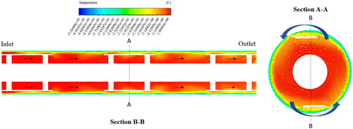
During the study, it was found that the temperature distribution in the ice cream mixture was not uniform throughout the space. Instead, there were areas where the temperature was significantly lower, particularly around the blades of the heat exchanger that scraped the surface of the tube. This may be due to the high velocity near the blades. The high velocity of the fluid, likely caused by the scraping action of the blades, enhances convective heat transfer, leading to a more efficient cooling effect. Therefore, these areas experience a greater reduction in temperature compared to other parts of the fluid, resulting in an inhomogeneous temperature distribution within the fluid. This study aligns with the research conducted by Yataghene and Legrand (2013) related to temperature distribution inside scraped surface heat exchangers.

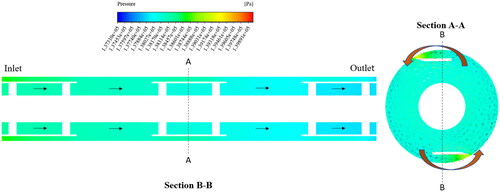
3.3.3. Pressure distribution

Figure 13 displays the variation of pressure as the mixture proceeds forward from the inlet to the outlet in a SSF (sectional plane B–B). A pressure drop can be observed between the inlet and outlet of the heat transfer tube. The mixture flow occurs from the region of high pressure to the region of low pressure and this is the reason flow takes place in the horizontal type SSF. The pressure distribution in the midplane of the freezer was also described with the help of sectional plane A–A. The normal distribution of pressure can be observed across the plane except for the region where the blade strikes close to the inner surface of the heat transfer tube wall. As soon as the flow strikes this region, the flow changes the direction which can be seen from the directional velocity vectors. The momentum accumulation in this region results in pressure increase and can be seen more where the blade tip encounters the wall. Whereas on the opposite of the blade, i.e. opposite to the outer surface of the blade, a normal pressure distribution can be seen.

Figure 13. Pressure distribution under reference operating conditions V̇_mix = 240 lph, T_R = −95 °C, and N_rotor =125 rpm in the sectional plane A–A (right side) and B–B (left side).

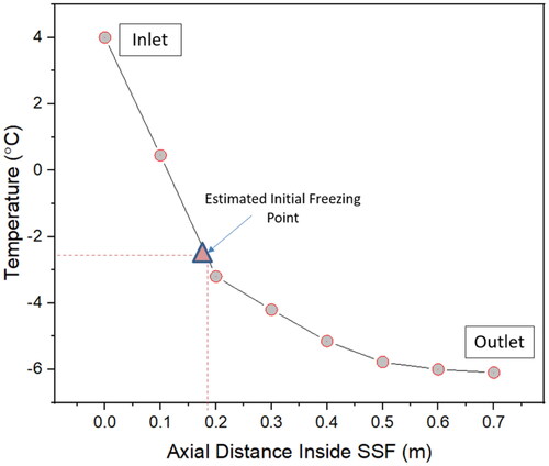
3.3.4. Temperature variation along axial distance of SSF

The temperature variation along the flow direction of the ice cream mixture was computed using an ANSYS fluent solver as shown in Figure 14. The CFD results were obtained for reference operating conditions V̇_mix = 240 lph, T_R = –95 °C, and N_rotor =125 rpm. The freezing point of the mixture according to the composition as computed earlier should be close to –2.72 °C. From the figure, it can be seen that on the basis of computational analysis, it was achieved at a distance close to 0.2 m. As the mixture flows from inlet to outlet, it can be seen from the graph that the temperature drops more slowly along the axial coordinate, once the initial freezing point is reached. This can be interpreted as higher energy requirements for freezing ice cream mixes once the initial freezing point is reached. Overall, the temperature drop in the axial direction of a scraped surface heat exchanger during cooling is a result of complex interactions between fluid dynamics, heat transfer mechanisms, and the design of the heat exchanger.

Figure 14. Temperature variation along axial distance of SSF for reference operating conditions V̇_mix = 240 lph, T_R = −95 °C, and N_rotor =125 rpm.

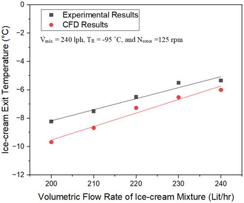
3.4. Validation of the experimental results

The drawing temperature obtained at different volumetric flow rates was compared with the results obtained experimentally as shown in Figure 15. Both the results were obtained under reference operating conditions. The experimental results were found to be in line with the CFD results. The difference in CFD and experimental results may be due to the losses during real experimentation that were not considered while computing CFD results.

Figure 15. Comparison of experimental and CFD results of ice cream exit temperature under reference operating conditions.

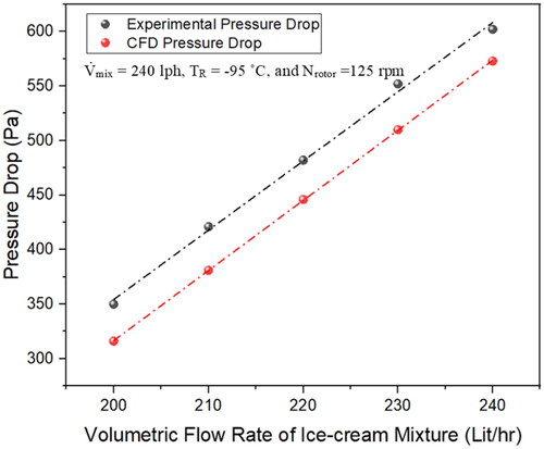
The pressure drop results obtained experimentally were also compared with the CFD results as can be seen from Figure 16. The pressure drop results were obtained under reference operating conditions. Both the results show the linear variation in pressure drop values with the change in the volumetric flow rate of the ice cream mixture.

Figure 16. Comparison of experimental and CFD pressure drop results while passing the ice cream mixture through SSF under reference operating conditions.

4. Conclusions

In this study, a thorough investigation of the performance of SSF in ice cream production was conducted through a combination of experimental investigation and CFD analysis. A distinct flow pattern characterized by confinement between the blades and the inner surface of the heat transfer tube, leading to accelerated temperature decrease due to recirculation effects, was observed. Moreover, numerical simulations identified the initial freezing point at an axial distance of 0.2 m within the SSF setup. The comparative analysis between experimental and CFD data demonstrated a maximum discrepancy of 2.5%, which was considered satisfactory. Beyond quantitative assessments, the significance of this research findings lies in their implications for sustainable development. Optimizing ice cream production through SSF not only enhances process economics but also has the potential to reduce energy consumption and environmental impact. In the present study, LN₂ was used for ice cream which is inert and non-toxic, posing minimal risk to the environment when used properly. It does not contribute to ozone depletion or greenhouse gas emissions, unlike some refrigerants used in conventional freezing systems. Rapid freezing with liquid nitrogen also helps preserve the quality and freshness of food products, reducing the likelihood of spoilage and food waste. In conclusion, the study provides valuable insights into the dynamics of SSF in ice cream production, offering opportunities for process optimization and sustainability.

Author contribution statement

Awani Shrivastav collected the data and wrote the manuscript; Tridib K. Goswami and Punyadarshini Punam Tripathy supervised the work and edited the manuscript; Chanchal Gupta and Suraj Kumar helped with the CFD simulation and analysis part of the manuscript.

Disclosure statement

No potential conflict of interest was reported by the author(s).

Data availability statement

All data used for this research is included in this manuscript.

Additional information

Funding

This research is funded by the Agriculture and Food Engineering Dept, IIT Kharagpur, India, (Institute ID: IR-O-U-0573)

Indian Institute of Technology Kharagpur;

Notes on contributors

Awani Shrivastav

Awani Shrivastav Ph.D. (IIT Kharagpur).

Tridib K. Goswami

Tridib K. Goswami Professor (IIT Kharagpur).

Punyadarshini Punam Tripathy

Punyadarshini Punam Tripathy Associate Professor (IIT Kharagpur).

Chanchal Gupta

Chanchal Gupta Scientist (CSIR-CMERI Centre of Excellence Farm Machinery (CoEFM), Ludhiana).

Suraj Kumar

Suraj Kumar Research Scholar (IIT Kharagpur).

References

- Ali, S., & Baccar, M. (2017). Numerical study of hydrodynamic and thermal behaviors in a scraped surface heat exchanger with helical ribbons. Applied Thermal Engineering, 111, 1069–1082. https://doi.org/10.1016/j.applthermaleng.2016.09.116
- Bahramparvar, M., & Mazaheri Tehrani, M. (2011a). Application and functions of stabilizers in ice cream. Food Reviews International, 27(4), 389–407. https://doi.org/10.1080/87559129.2011.563399
- Boccardi, G., Celata, G. P., Lazzarini, R., Saraceno, L., & Trinchieri, R. (2010). Development of a heat transfer correlation for a scraped-surface heat exchanger. Applied Thermal Engineering, 30(10), 1101–1106. https://doi.org/10.1016/j.applthermaleng.2010.01.023
- Boccardi, G., Celata, G. P., Lazzarini, R., Saraceno, L., & Trinchieri, R. (2008). Development of a heat exchange correlation in the presence of an agitator. In Proceedings of 5th European Thermal-Sciences Conference.
- Chen, C. S. (1985). Thermodynamic analysis of the freezing and thawing of foods. Journal of Food Science, 50(4), 1158–1162. https://doi.org/10.1111/j.1365-2621.1985.tb13034.x
- Choi, Y., & Okos, M. R. (1986). Effects of temperature and composition on the thermal properties of foods. In Le M. Maguer, & P. Jelen (Eds.), Food Engineering and Process Applications, Vol. 1: Transport Phenomena (pp. 93–101). New York: Elsevier.
- De Goede, R., & De Jong, E. J. (1993). Heat transfer properties of a scraped-surface heat exchanger in the turbulent flow regime. Chemical Engineering Science, 48(8), 1393–1404. https://doi.org/10.1016/0009-2509(93)80046-s
- Duffy, B. R., Wilson, S. K., & Lee, M. E. M. (2007). A mathematical model of fluid flow in a scraped-surface heat exchanger. Journal of Engineering Mathematics, 57(4), 381–405. ISSN 00220833 https://doi.org/10.1007/s10665-006-9116-4
- Harriott, P. (1959). Heat transfer in scraped surface exchangers. American Institute of Chemical Engineers Symposium Series, 55(29), 137–139.
- Hernández-Parra, O. D., Plana-Fattori, A., Alvarez, G., Ndoye, F.-T., Benkhelifa, H., & Flick, D. (2018). Modeling flow and heat transfer in a scraped surface heat exchanger during the production of sorbet. Journal of Food Engineering, 221, 54–69. https://doi.org/10.1016/j.jfoodeng.2017.09.027
- Huggins, F. E. (1931). Effect of scrapers on heating, cooling and mixing. Industrial & Engineering Chemistry, 23(7), 749–753. https://doi.org/10.1021/ie50259a005
- Kim, J., Chun, H. H., Park, S., Choi, D., Choi, S. R., Oh, S., & Yoo, S. M. (2014). System design and performance analysis of a quick freezer using supercooling. Journal of Biosystems Engineering, 39(4), 330–335. https://doi.org/10.5307/JBE.2014.39.4.330
- Kool, J. (1958). Heat transfer in scraped vessels and pipes handling viscous material. Transactions of the Institution of Chemical Engineers, 36(4), 253–258.
- Kumar, Y., Tiwari, S., & Kumar, Y, Lecturer, Department of Food Processing &Technology, Bilaspur University, C.G., India. (2018). Cryogenic freezing technology. International Journal of Pure & Applied Bioscience, 6(2), 1343–1346. https://doi.org/10.18782/2320-7051.6458
- Lakhdar, M. B., Cerecero, R., Alvarez, G., Guilpart, J., Flick, D., & Lallemand, A. (2005). Heat transfer with freezing in a scraped surface heat exchanger. Applied Thermal Engineering, 25(1), 45–60. https://doi.org/10.1016/j.applthermaleng.2004.05.007
- Latinen, G. A., & Skelland, A. H. (1959). Discussion of the paper: Correlation of scraped film heat transfer in the votator by. Chemical Engineering Science, 9(4), 263–266. https://doi.org/10.1016/0009-2509(59)85008-9
- Lee, J. H., & Singh, R. K. (1990). Mathematical models of scraped-surface heat exchangers in relation to food sterilization. Chemical Engineering Communications, 87(1), 21–51. https://doi.org/10.1080/00986449008940682
- Mukesh Kumar, P. C., & Chandrasekar, M. (2019). CFD analysis on heat and flow characteristics of double helically coiled tube heat exchanger handling MWCNT/water nanofluids. Heliyon, 5(7), e02030. https://doi.org/10.1016/j.heliyon.2019.e02030
- Penney, W. R., & Bell, K. J. (1967). Correction-close-clearance agitators-part 1. Power requirements. Industrial & Engineering Chemistry, 59(6), 17–17. https://doi.org/10.1021/ie50690a601
- Qin, F., Chen, X. D., Ramachandra, S., & Free, K. (2006). Heat transfer and power consumption in a scraped-surface heat exchanger while freezing aqueous solutions. Separation and Purification Technology, 48(2), 150–158. https://doi.org/10.1016/j.seppur.2005.07.018
- Qin, F. G., Chen, X. D., & Russell, A. B. (2003). Heat transfer at the subcooled-scraped surface with/without phase change. AIChE Journal, 49(8), 1947–1955. https://doi.org/10.1002/aic.690490804
- Saraceno, L., Boccardi, G., Celata, G. P., Lazzarini, R., & Trinchieri, R. (2011). Development of two heat transfer correlations for a scraped surface heat exchanger in an ice-cream machine. Applied Thermal Engineering, 31(17-18), 4106–4112. https://doi.org/10.1016/j.applthermaleng.2011.08.022
- Shrivastav, A., & Goswami, T. (2018). Conventional industrial ice cream freezers and its thermal design: a review. Journal of Food Science and Nutrition, 01(01), 21–28. https://doi.org/10.35841/food-science.1.1.21-28
- Shrivastav, A., Goswami, T. K., & Kotra, S. V. (2022). Rheological and adaptive neuro-fuzzy inference system (ANFIS) modeling of ice cream at different gelatin concentrations produced by liquid nitrogen infusion technique. Journal of Biosystems Engineering, 47(3), 344–357. https://doi.org/10.1007/s42853-022-00151-z
- Skelland, A. H. P. (1958). Correlation of scraped-film heat transfer in the votator. Chemical Engineering Science, 7(3), 166–175. https://doi.org/10.1016/0009-2509(58)80023-8
- Skelland, A. H. P., Oliver, D. R., & Tooke, S. (1962). Heat transfer in a water-cooled scraped surface heat exchanger. British Chemical Engineering, 7, 346–353.
- Szpicer, A., Bińkowska, W., Wojtasik-Kalinowska, I., Salih, S. M., & Półtorak, A. (2023). Application of computational fluid dynamics simulations in food industry. European Food Research and Technology, 249(6), 1411–1430. https://doi.org/10.1007/s00217-023-04231-y
- Tiwari, A. K., Ghosh, P., Sarkar, J., Dahiya, H., & Parekh, J. (2014). Numerical investigation of heat transfer and fluid flow in plate heat exchanger using nanofluids. International Journal of Thermal Sciences, 85, 93–103. https://doi.org/10.1016/j.ijthermalsci.2014.06.015
- Trommelen, A. M., Beek, W. J., & Van De Westelaken, H. C. (1971). A mechanism for heat transfer in a votator-type scraped-surface heat exchanger. Chemical Engineering Science, 26(12), 1987–2001. https://doi.org/10.1016/0009-2509(71)80037-4
- Varga, T., Szepesi, G., & Siménfalvi, Z. (2017). Horizontal scraped surface heat exchanger—experimental measurements and numerical analysis. Pollack Periodica, 12(1), 107–122. https://doi.org/10.1556/606.2017.12.1.9
- Yataghene, M., & Legrand, J. (2013). A 3D-CFD model thermal analysis within a scraped surface heat exchanger. Computers & Fluids, 71, 380–399. https://doi.org/10.1016/j.compfluid.2012.10.026
- Yataghene, M., Pruvost, J., Fayolle, F., & Legrand, J. (2008). CFD analysis of the flow pattern and local shear rate in a scraped surface heat exchanger. Chemical Engineering and Processing: Process Intensification, 47(9-10), 1550–1561. https://doi.org/10.1016/j.cep.2007.07.009
- Zhu, Z., Zhou, Q., & Sun, D.-W. (2019). Measuring and controlling ice crystallization in frozen foods: A review of recent developments. Trends in Food Science & Technology, 90, 13–25. https://doi.org/10.1016/j.tifs.2019.05.012